Process Simulation in Excel for a
Quantitative Management Course
Raymond R. Hill
Department of Operational Sciences Air Force Institute of Technology Wright-Patterson AFB, OH 45424
[email protected] Abstract
A nagging limitation of teaching spreadsheet-based quantitative decision-making courses is the some-times stilted view of simulation presented, a view that overly emphasizes sampling simulation at the expense of process simulation. Without a viable spreadsheet-based process simulation package, the best efforts aimed at overcoming this emphasis on sampling simulation have provided passing refer-ences to special purpose simulation packages focused on process simulation. We introduce and discuss SimQuick as an alternative approach for teaching process simulation within the context of a spread-sheet-based approach to teaching simulation. Al-though an early tool, and somewhat limited when compared to special purpose simulation packages, SimQuick provides a viable means for teaching the process of simulation modeling and reinforcing the salient features of process modeling as a quantita-tive technique.
Disclaimer:The views expressed in this article are those of the authors and do not reflect the official policy of the United States Air Force, Department of Defense, or the US Government.
Introduction
A nagging limitation of teaching spreadsheet-based modeling is providing sufficient coverage of simu-lation. Simulation is an important quantitative tech-nique but spreadsheet-based approaches sometimes ignore a good portion of the technique. Basic
spread-sheet capabilities are very good for sampling lation methods but ill suited for discrete-event simu-lation. This paper proposes and discusses how to use SimQuick, an Excel-based simulation package, to overcome these limitations and bring discrete-event simulation into the spreadsheet-based quanti-tative management course.
A simulation is a computer model used to evaluate a system numerically (Law and Kelton, 2000). Sto-chastic simulations involve random variates to model variables assumed to follow some probability dis-tribution. When the simulation explicitly models a system as that system changes over time, the simu-lation is referred to as a dynamic simusimu-lation. Recent surveys list simulation as among the most popular and widely used operational research techniques (Lane, et al., 1993).
Spreadsheets have long been in use in the business world while unfortunately ignored among some ana-lysts and engineers. That tendency is rapidly falling away as the modern spreadsheet truly provides a diverse and robust environment for most modeling needs. The modern spreadsheet provides a means to store and manage data, run statistical analyses, con-duct mathematical modeling, import and export tables and graphs, and interface to other more pow-erful computer packages. In short, the spreadsheet is a (nearly) complete analytical toolbox.
Not surprisingly, quantitative management texts fo-cused on surveying quantitative techniques have nearly unanimously adopted the spreadsheet as the computing platform of choice. The benefits provided the course instructor include:
•
pre-existing familiarization with the platform; and•
increased likelihood of student future use of the quantitative techniquesTeaching new concepts, such as is often the case in courses involving quantitative techniques, is facili-tated by the students’ immediate grasp of the com-puter tool. The instructor challenge then becomes one of expanding the students’ abilities to under-stand and apply the quantitative methods. Then, because the spreadsheet is so widely available, and
if the instructor has made the proper academic-to-application connection, the graduated student may find their problems amenable to spreadsheet model-ing and actually use the techniques in practice. The spreadsheet platform also introduces challenges for the instructor. These include:
•
differences between mathematical formulation and spreadsheet paradigms;•
too much modeling freedom; and•
limited view of the breadth and depth of quan-titative modeling.The spreadsheet paradigm is one of arrays and ma-trices of values but not necessarily matrix algebra. Mathematical models are usually algebraic in rep-resentation. The instructor needs to help the student build the mental mapping between the two para-digms. The spreadsheet also imposes few limitations on how a user chooses to design a worksheet. This freedom is carried over into the design and specifi-cation of quantitative models. Such expressive free-dom can be a source of confusion to the novice mod-eler. The instructor must avoid overwhelming the student with spreadsheet capabilities and focus on effective quantitative modeling methodology. This expressive freedom can be particularly troublesome when correct answers are obtained using question-able modeling methods or when the correct spread-sheet model bears no resemblance to an associated mathematical formulation.
The spreadsheet is a viable modeling platform but has limitations, in breadth of technique supported and in the size of models accepted. Advanced users can of course significantly extend spreadsheet ca-pabilities (like in Excel) with special purpose pro-gramming (like VBA), but such topics generally fall outside the scope of quantitative courses. The sur-vey course student will generally remain a novice user of quantitative management tools. Thus, the survey course should provide a basic understanding of a range of techniques, a sufficient understanding of the technique’s salient features, and most impor-tantly, an appreciation of what is still unfamiliar with respect to the technique.
Simulation on Spreadsheets
Analytical simulation falls into two broad catego-ries:
•
sampling or Monte Carlo simulation, and•
process simulation (or discrete-eventsimula-tion).
Evans (2001) described these as Monte Carlo or risk simulation and systems simulation, respectively. Other simulation applications, such as human-in-the-loop, distributed, web-based, and training simula-tions are excluded from the present discussion. Sampling simulation applications are perfect for the spreadsheet. Sampling simulation is used to exam-ine risk or uncertainty associated with static models or simulations that involve activity-scanning ap-proaches. Typical models might be investment mod-els, inventory modmod-els, even fairly simply queuing models are manageable in the spreadsheet (Ragsdale, 2001; Camm and Evans, 1996). The spreadsheet easily recalculates a model, spreadsheet functions provide random number generators, and the spread-sheet has plenty of capability to save and analyze the simulation data generated. Nearly all manage-ment science texts include a chapter on simulation, a chapter usually focused on sampling simulation. Add-ins like @Risk and Crystal Ball significantly increase one’s ability to conduct, and teach, sam-pling simulation, as well as conduct risk analysis in simulation studies or student projects and theses. Process simulation for spreadsheets are not quite as applicable. Process simulation is used to capture complex system state changes over time, particu-larly when the state changes are defined by events within the system. The dynamic interactions and uncertain event ordering are difficult to capture in a spreadsheet model without somehow augmenting spreadsheet capabilities. Typical examples might include maintenance operations involving demands on limited resources and unpredictable failure events, production processes involving looping within the various workstations within the facility, or even complex combat models with multiple in-teracting systems engaged in conflict. These more complicated, and often more realistic, simulation applications are either not discussed or just briefly
mentioned when referencing the more sophisticated simulation packages. Exceptions include Camm and Evans (1996), Evans and Olsen (1998), and Laurence and Pasternack (1998) whose works include student versions of these more powerful packages. These exceptions are, however, admittedly limited in the amount of time and space devoted to discussing how to use these more powerful simulation packages. A stilted view of simulation due to spreadsheet limitations deprives the survey-course student a full appreciation of the power and benefits of the simu-lation as a quantitative technique. To overcome this limitation, we incorporated SimQuick into the simu-lation portion of our survey course. In our case, process simulation follows sampling simulation for which we use Crystal Ball. See Evans (2000) or Ragsdale (2001) for details on sampling simulation using Crystal Ball.
SimQuick Introduced
SimQuick (Hartvigsen, 2001) is a process-oriented simulation package for Excel. SimQuick is not an Excel add-in (such as an .xla file) but rather a spread-sheet template in which a user specifies the elements of a simulation model, the parameterization of those
elements, and the connections between the elements. These specifications are indicated to SimQuick via particular worksheet tables whose access is con-trolled via VBA menus within the SimQuick spread-sheet. SimQuick can be described as a first-genera-tion package, replete with significant limitafirst-genera-tions when compared to mature, special purpose pack-ages such as Extend, AweSim, ProModel, or Arena. However, we have found SimQuick, despite its limi-tations, quite adequate in providing a spreadsheet tool with which to focus on the salient features of process simulation thereby providing more complete coverage of simulation as a quantitative technique. Figure 1 displays the SimQuick control panel. Each button transfers control to a worksheet containing the SimQuick tables through which one specifies a simulation. The only elements available in SimQuick are those listed on the panel, and described below. This limitation on SimQuick constructs is a bless-ing for the survey course as the student must focus on the process of simulation modeling to success-fully employ SimQuick. Further, the student is not overwhelmed by the large number of modeling constructs such as one finds in the special purpose simulation packages. The instructor must however choose modeling projects that are appropriate for the SimQuick package.
Process of Simulation Modeling
A frustrating aspect of teaching simulation, whether a component within a survey course, or a full-fledged simulation course, is reminding students that simu-lation is applied statistics. Stochastic simusimu-lation output is a function of input random variables and thus also a random variable and statistics are the language of random variables. The simulation model is not the end result, but rather a tool one builds within the simulation process. The true end product of a simulation effort, just as in a mathematical modeling effort, is insight into the system or pro-cess under study, insight gained, in this case, via statistical analysis of simulation output. The SimQuick design provides a focus on the simula-tion process.
Hartvigsen (2001) lists three steps in using SimQuick:
1. Conceptually build a model of the process; 2. Enter the model into SimQuick;
3. Test process improvement ideas with the model
We expand the first step quite a bit when teaching process simulation with SimQuick to focus more on the methodology of simulation. This includes in-creasing the specificity contained within a concep-tual model. This facilitates the second step as enter-ing a model into SimQuick is very straightforward but does require the up-front planning during the conceptual modeling building process.
Evans (2000) offers the following four step ap-proach:
1. Formulate the problem to include defining ob-jectives, measurements, and scenarios; 2. Develop a logical model;
3. Specify probabilistic assumptions; and 4. Implement model on computer.
Evans’ four-step approach is closer to our needs al-though additional emphasis is given to verifying and validating the logical model before implementing the model into SimQuick. This is due to the increased complexity of a process model versus a static model as built for a sampling simulation application. We can use Step 3 to tie back to Crystal Ball, and sam-pling simulation, through the use of Crystal Ball’s distribution fitting capabilities to analyze historical data from which to derive representative probabil-ity distributions.
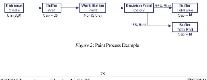
A simple flow-chart augmented with additional syn-tax provides a simple, easy to learn and intuitive simulation process. Figure 2 is a very simple con-ceptual model intended to motivate our approach to teaching simulation. In this example, entities arrive, wait for a paint station, are painted Red or Blue, and once painted leave the system. We want to count how many are painted so we use two buffers, Total Red and Total Blue. The flowchart elements in Fig-ure 2 list the corresponding SimQuick element type, a unique name for the element, and any other data required by the SimQuick element. Linkages among the elements are indicated by the directed arcs and specified to SimQuick via the unique names assigned the element. Figure 2 contains sufficient detail to directly specify the model to SimQuick. This flow-chart in Figure 2 was drawn using the cell format-ting and the line drawing facilities within Excel.
SimQuick Limitations
SimQuick represents a new and initial capability for process simulation within Excel. Not surprisingly SimQuick has limitations. Understanding and ac-commodating these limitations helps realize the ben-efits SimQuick brings to the classroom.
SimQuick elements are defined via tables within worksheets of the SimQuick workbook. The tables currently allow up to 20 elements of each type. Simu-lations are limited to 10,000 time units and 100 in-dependent replications. There is no facility for re-moving transient data nor can one specify random number streams. There is also a limited choice of probability distributions although those implemented are quite commonly used in simulation.
Like more powerful packages, SimQuick drops en-tities if those enen-tities have no place to move or wait. Resource usage is prioritized by the order in which workstations are defined in the Workstation worksheet and workstations handle as many entities as resources allow. SimQuick will also do initial er-ror checking before executing the simulation.
SimQuick Teaching Tips
SimQuick limitations mean certain things cannot be easily modeled. Just like any programming language, and all simulation packages are programming lan-guages, one must learn to manipulate the language properly to obtain the desired modeling effect. The following are some initial lessons learned.
•
Emphasize the importance of fully understand-ing the system under study and then mappunderstand-ing the desired conceptual model onto the SimQuick syntax when creating the actual simulation model.•
Emphasize the importance of fully specifying the flowchart model and uniquely naming each piece in the model.•
Use buffers for each workstation. An object will drop from the simulation if not buffered.•
Emphasize the need to carefully read and grasp how SimQuick interprets connections betweenelements. For instance, two buffers feeding a common workstation produces a combine object effect.
•
More than two decision points requires plac-ing SimQuick decision point elements in se-quence and determining the correct condi-tional probabilities.Fortunately, each “limitation” of SimQuick provides an opportunity to reinforce two key concepts to the student: structured walk through of models for vali-dation, and modeling for effect. A structured walk-through is usually associated with software engineer-ing but serves the novice modeler well to reinforce the notion that a simulation, like any computer pro-gram it is, will only do what is specified, not neces-sarily what the modeler thinks it will accomplish. Modeling effects deals with using the structure and syntax of the language in such a way that the result-ing model sufficiently mimics the intended pro-cess—the output data makes sense. For example, a maintenance process simulation can capture the ef-fect of maintainer transient time, without explicitly modeling maintainer travel, by properly incorporat-ing travel time into maintenance repair times.
SimQuick Example
Consider the following example:
Two components arrive simultaneously, A and B. All components are polished. Part B must be inspected and if required, sanded and re-polished. Completed A and B components are paired and assembled into a finished compo-nent, Z. Finished components are placed in holding racks until an hourly delivery truck arrives to cart off the components. The deliv-ery trucks have limited storage, handling up to 15 finished components per pickup.
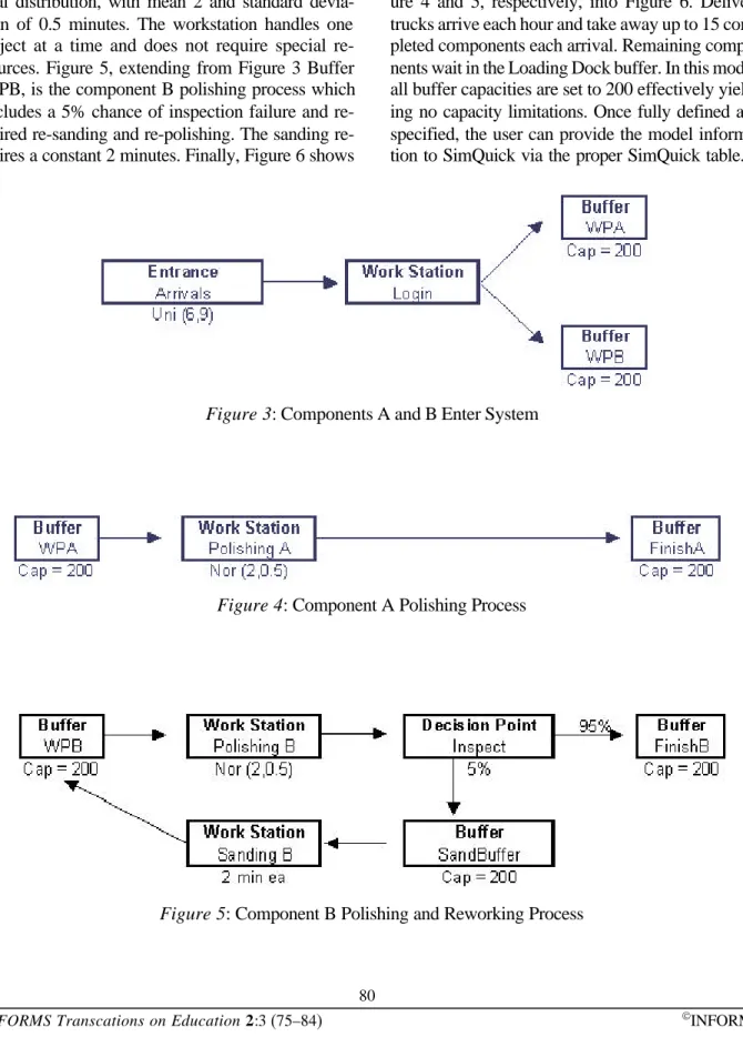
The complete flowchart for this example cannot fit neatly in single page. Figures 3-6 contain the com-ponents of the final flowchart. The reader will note common elements in the figures. These common elements are the connecting points between the fig-ures. Figure 3 shows an object entrance and a split
into two components, A and B, each moving into a Buffer to await polishing. Figure 4, extending from Figure 3 Buffer WPA, is the component A polishing process. The polishing process time follows a nor-mal distribution, with mean 2 and standard devia-tion of 0.5 minutes. The workstadevia-tion handles one object at a time and does not require special re-sources. Figure 5, extending from Figure 3 Buffer WPB, is the component B polishing process which includes a 5% chance of inspection failure and quired sanding and polishing. The sanding re-quires a constant 2 minutes. Finally, Figure 6 shows
the final assembly process. Objects from Buffers FinishA and FinishB combine to form the final prod-uct, Z, an operation that requires 1.5 minutes. These buffers are also the connecting points between Fig-ure 4 and 5, respectively, into FigFig-ure 6. Delivery trucks arrive each hour and take away up to 15 com-pleted components each arrival. Remaining compo-nents wait in the Loading Dock buffer. In this model, all buffer capacities are set to 200 effectively yield-ing no capacity limitations. Once fully defined and specified, the user can provide the model informa-tion to SimQuick via the proper SimQuick table.
Figure 5: Component B Polishing and Reworking Process
Figure 3: Components A and B Enter System
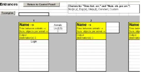
Figure 7 is a partial screen shot showing the En-trance element (included in Figure 3), named Ar-rive, as specified to SimQuick. Note the Entrances worksheet provides guidance on the acceptable in-ter-arrival and number of objects arriving distribu-tions, to include a constant value. Similar help is
presented on other worksheets. The Examples but-ton provides precisely that, an example completed table. In this model, the time between arrivals is modeled as a uniform random variable between 6 and 9 time minutes. A single object arrives and moves directly to the Login (workstation) element.
Figure 6: Final Assembly and Packaging Processes
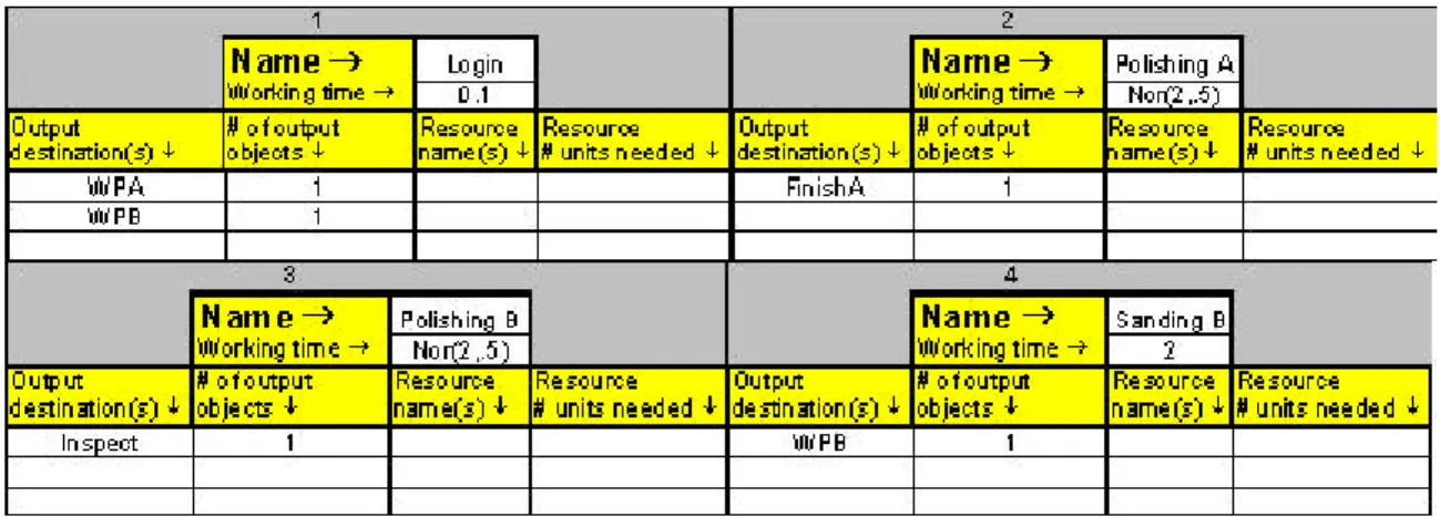
Figure 8 is a collage from four of the five tables in which the conceptual model workstations are speci-fied to SimQuick. These tables specify the worksta-tions from Figures 3-5. Note each element has a unique Name, the processing time may be a con-stant (0.1 or 2) or some random amount of time
(Nor(2,.5)), and the destination for once processing is completed is specified. In the case of the Login workstation, a nominal time is given while the dual output destinations serve to split the single arrival into two components, A and B (since these arrive simultaneously.)
Figure 9 contains a collage of all the buffer elements defined in the model. Each buffer is provided a ca-pacity (use a large number if caca-pacity is not an is-sue) and each buffer starts empty. Each element is provided a unique name and lists a single output
destination. The name specified in the output desti-nation ties directly to the directed arc used in the model flowchart in Figures 3-6. To conserve space, neither the Decision Point element nor the Exit ele-ments are shown.
Figure 8:Specification of Four of Five Workstation Elements
Once the elements are specified to SimQuick, the number of replications and length of each simula-tion are provided. When the Run Simulasimula-tion button is selected, SimQuick does some error checking and if all passes, conducts the simulation. The results of each simulation run, along with cumulative statis-tics are written to another worksheet accessible via the View Results button (see Figure 1).
SimQuick does not currently provide a means to specify output measures, the user gets what SimQuick provides. However, SimQuick does
pro-vide the data for each of the simulation replications, data which can be easily copied and further analyzed using Excel statistical analysis tools. In the case of this re-working example, workstation and delivery truck utilization results (not included) indicate a woefully underutilized process (as one might expect by examining the system description.)
SimQuick Output
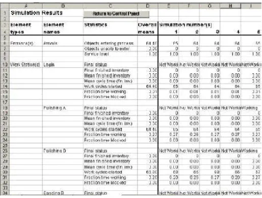
Figure 10 is a snapshot of the SimQuick output panel. SimQuick output is predefined; SimQuick provides general data on each element contained within the
model. Inferences for the system are based on this data provided.
As indicated in Figure 10, SimQuick provides the data for each replication and a summary average across all the replications. Variance information re-quires the user save the results worksheet and use Excel functions to calculate variance information based on the replication data. For this model, across the ten replications, an average of 64.4 components arrive. The Polishing workstations are utilized
ap-proximately 27% of the time (Fraction time work-ing) and we can infer that 2.4 items required sand-ing (difference in Work Cycles started for Polishsand-ing A versus Polishing B as well as the Work cycles started for Sanding B). This represents a 3.7% fail rate which is very close to the 5% theoretical fail rate specified for the model. Other data provided (not shown) indicate a 1% utilization of the Sander workstation and only 47% of the delivery truck ca-pacity is employed. In class, various embellishments can be included and the resulting system impacts
examined using the output from separate SimQuick runs.
Concluding Remarks
In our class, we introduce SimQuick and process simulation after presenting sampling simulation us-ing Crystal Ball. Our focus has been on the process of simulation and in particular developing accuracy in defining the flowchart model of the process. Stu-dent feedback has been positive particularly in the ease of use of SimQuick once the process model is defined. More importantly, we were able to provide a familiarization of simulation that balances both sampling and process simulation.
Spreadsheets are uniquely suited for sampling simu-lation and it is quite logical for spreadsheet-based texts to focus on sampling simulation. As educators however we must provide simulation familiarization across the breadth of the analytical simulation spec-trum. While limited in capabilities, SimQuick pro-vides a useful spreadsheet-based vehicle for comple-menting products like Crystal Ball or @Risk and thus providing a relatively thorough familiarization of simulation.
References:
Camm, J. and J. R. Evans. (1996). Management Science: Modeling, Analysis and Interpretation,
South-Western, Cincinnati, Ohio.
Evans, J. R. and D. L. Olsen. (1998). Introduction to Simulation and Risk Analysis, Prentice-Hall, Upper Saddle River, NJ.
Evans, J.R. (2000), “Spreadsheets as a Tool for Teaching Simulation,” INFORMS Transactions on Education , Vol. 1, No. 1, http://ite.informs.org/ Vol1No1/evans/evans.html
Hartvigsen, David. (2001). SimQuick: Process Modeling with Excel, Prentice-Hall, Upper Saddle River, NJ.
Lane, M. S., A. H. Mansour, and J. L. Harpell. (1993). “Operations Research Techniques: A Longitudinal Update, 1973-1988,” Interfaces, Vol. 23, No. 2, pp. 63-68.
Laurence, J. A. and B. A. Pasternak. (1998).
Applied Management Science: A Computer-Integrated Approach for Decision Making, John Wiley & Sons, New York.
Law, A. M. and W. D. Kelton. (2000). Simulation Modeling and Analysis, Third Edition, McGraw-Hill, New York.
Ragsdale, C. T. (2001). Spreadsheet Modeling and Decision Analysis: A Practical Introduction to Management Science. South-Western, Cincinnati, Ohio.
Winston, W. L. and S. C. Albright. (1997). Practi-cal Management Science: Spreadsheet Modeling and Applications, Duxbury, Belmont, CA