in Parametric Markov Decision Processes
Tobias Winkler
RWTH Aachen University, Germany [email protected]
Sebastian Junges
RWTH Aachen University, Germany [email protected]
Guillermo A. Pérez
University of Antwerp, Belgium [email protected]Joost-Pieter Katoen
RWTH Aachen University, Germany [email protected]
Abstract
This paper studies parametric Markov decision processes (pMDPs), an extension to Markov decision processes (MDPs) where transitions probabilities are described by polynomials over a finite set of parameters. Fixing values for all parameters yields MDPs. In particular, this paper studies the complexity of finding values for these parameters such that the induced MDP satisfies some reachability constraints. We discuss different variants depending on the comparison operator in the constraints and the domain of the parameter values. We improve all known lower bounds for this problem, and notably provide ETR-completeness results for distinct variants of this problem. Furthermore, we provide insights in the functions describing the induced reachability probabilities, and how pMDPs generalise concurrent stochastic reachability games.
2012 ACM Subject Classification Theory of computation→Probabilistic computation; Theory of computation→Logic and verification; Theory of computation→Markov decision processes
Keywords and phrases Parametric Markov decision processes, Formal verification, ETR, Complexity
Digital Object Identifier 10.4230/LIPIcs.CONCUR.2019.14
Related Version https://arxiv.org/abs/1904.01503
Funding This work has been supported by the DFG RTG 2236 “UnRAVeL”, and the ERC Advanced Grant 787914 “FRAPPANT”.
Acknowledgements We would like to thank Krishnendu Chatterjee for his pointer to CSRGs.
1
Introduction
Markov decision processes (MDPs) arethe model to reason about sequential processes under (stochastic) uncertainty and determinism. Markov chains (MCs) are MDPs without non-determinism. Often, probability distributions in these models are difficult to assess precisely during design time of a system. This shortcoming has led to interval MCs [15, 35, 50, 54] and interval MDPs (also known as Bounded-parameter MDPs) [27, 42, 58], which allow for interval-labelled transitions. Analysis under interval Markov models is often too pessimistic: The actual probabilities on the transitions are considered to be non-deterministically and locally chosen. Intuitively, consider the probability of a coin-flip yielding heads in some stochastic environment. In interval models, the probability may vary with the local memory state of an agent acting in this environment. Such behaviour is unrealistic. Parametric
© Tobias Winkler, Sebastian Junges, Guillermo A. Pérez, and Joost-Pieter Katoen; licensed under Creative Commons License CC-BY
MCs/MDPs [19, 23, 28, 39] (pMCs, pMDPs) overcome this limitation by adding dependencies (or couplings) between various transitions – they add global restrictions to the selection of the probability distributions. Intuitively, the probability of flipping heads can be arbitrary, but should be independent of an agent’s local memory. Such couplings are similar to restrictions on schedulers in decentralised/partially observable MDPs, considered in e.g., [5, 26, 51].
Technically, pMDPs label their transitions with polynomials over a finite set of parameters. Fixing all parameter values yields MDPs. The synthesis problem considered in this paper asks to find parameter values such that the induced MDPs satisfy reachability constraints. Such reachability constraints state that the probability – under some/all possible ways to resolve non-determinism in the MDP – to reach a target state is (strictly) above or below a threshold. A sample synthesis problem is thus: “Are there parameter values such that for all possible ways to resolve the non-determinism, the probability to reach a target state exceeds
1
2?” Variants of the synthesis problem are obtained by varying the reachability constraints,
and the domain of the parameter values. Parameter synthesis is supported by the model checkers PRISM [38] and Storm [22], and dedicated tools PARAM [29] and PROPhESY [21]. The complexity of the decision problems corresponding to parameter synthesis is mostly open. This paper significantly extends complexity results for parameter synthesis in pMCs and pMDPs. Table 1 on page 5 gives an overview of new results: Most prominently, it establishes ETR-completeness of reachability problems for pMCs with non-strict comparison operators, and establishes NP-hardness for pMCs with strict comparison operators. For pMDPs with demonic non-determinism, it establishes ETR-completeness for any comparison operator. For angelic non-determinism, mostly the synthesis problems are equivalent to their pMC counterparts. When considering pMDPs with a fixed number of variables, we establish uniform NP upper bounds for parameter synthesis under angelic or demonic non-determinism. These results are partially based on properties of pMDPs scattered in earlier work, and use a strong connection between polynomial inequalities and parameter synthesis.
Finally, pMDPs are interesting generalisations of other models: [37] shows that parameter synthesis in pMCs is equivalent to the synthesis of finite-state controllers (with a-priori fixed bounds) of partially observable MDPs (POMDPs) [46] under reachability constraints. Thus, as a side product we improve complexity bounds [10, 56] for (a-priori fixed) memory bounded strategies in POMDPs. In this paper, we show how pMDPs generalise concurrent stochastic reachability games [12, 20, 52]. We finish the paper by drawing some connections with robust schedulers, i.e. the question of how to optimally resolve non-determinism taking into account the uncertainty in the stochastic dynamics. Proofs are given in the related technical report.
Related work. Various results in this paper extend work by Chonev [16], who studied a model of augmented interval Markov chains. These coincide with parametric Markov chains. The work also builds upon results by Hutschenreiteret al.[33], in particular upon the result that pMCs with an a-priori fixed number of parameters can be checked in P. Furthermore, they study the complexity of PCTL model checking of pMCs. The complexity of finite-state controller synthesis in POMDPs has been studied in [10, 56]. Some of the proofs for ETR-completeness presented here reuse ideas from [48].
Methods (and implementations) to analyse pMCs by computing their characteristic solution function are considered in [19, 21, 23–25, 29, 33, 34]. Sampling-based approaches to find feasible instantiations in pMDPs are considered by [14, 28], while [3, 18] utilise optimisation methods. Finally, [44] presents a method to prove the absence of solutions in pMDPs by iteratively considering simple stochastic games [17]. Some other works on Markov models with structurally equivalent yet parameterised dynamics include [8, 9, 13, 53]. Parameter synthesis with statistical guarantees has been explored in, e.g., [6]. Further work on parameter synthesis in Markov models has been surveyed in [36].
2
Preliminaries
LetX be a finite set of variables. LetQ[X] andQ(X) denote the set of all rational-coefficient polynomial and rational functions on X, respectively. A rational function f /g can be represented as a pair (f, g) of polynomials. In turn, a polynomial can be represented as a sum of terms, where each term is given by acoefficient and a monomial. The (total) degree of a polynomial is the maximum over the sum of the exponents in the monomials. A polynomial is quadratic (respectively, quadric), if its total degree is two (four) or less. For a rational functionf(x1, . . . , xk)∈Q(X) and an instantiationval: X→Rwe writef[val] for the value
f(val(x1), . . . ,val(xk)). We use./to denote either of{≤, <,≥, >}and for either {≥, >}
(andanalogously). With./, we denote the complement, e.g. ≤ =>.
Consider a finite set S. Let Distr(S) denote the set of all distributions over S, and supp(δ)⊆S the support{s∈S |δ(s)>0} of distributionδ∈Distr(S).
2.1
Parametric Markov models
IDefinition 1(pMDP). Aparametric Markov Decision ProcessMis a tuple(S, X,Act, sι, P) with S a (finite) set of states, X a finite set of parameters, Act a finite set of actions,
sι∈S the initial state, andP:S×Act×S→Q[X]∪Rthe probabilistic transition function. Parameter-free pMDPs coincide with standard MDPs, as in [43]. We defineAct(s) ={a∈
Act| ∃s0∈S. P(s, a, s0)6= 0}. If|Act(s)|= 1 for alls∈S, thenMis aparametric Markov chain (pMC). We denote its transitions withP(s, s0) and omit the actions.
A pMDP issimple if and only if non-constant probabilities labelling transitions (s, a, s0) are of the form xor 1−x, and the sum of outgoing transitions from a state-action pair always is (equivalent to) 1. Formally, simple pMDPs satisfy the following two properties:
P(s, a, s0)∈ {x,1−x | x∈X} ∪Rfor alls, s0∈S anda∈Act; and P
s0∈SP(s, a, s0) = 1 for alls∈S anda∈Act(s).
I Definition 2 (Instantiation). Let M = (S, X,Act, sι, P) be a pMDP. An instantiation val:X →Ris well-definedif the induced functionsP(s, a,·)are distributions over S, i.e.
∀s, s0 ∈S,∀a∈Act.0≤P(s, a, s0)[val]∈R∧
X
ˆ
s∈S
P(s, a,sˆ)[val] = 1.
Let M[val] denote the parameter-free MDP in which P(s, a, s0) has been replaced by P(s, a, s0)[val]. We denote with P=0val := {(s, a, s0) ∈ S ×Act×S | P(s, a, s0) 6= 0∧
P(s, a, s0)[val] = 0} the transitions of M that become 0 in M[val]. A well-defined in-stantiationval isgraph-preserving if the topology of the pMDP is preserved, i.e. ifPval
=0 =∅.
The (well-defined) parameter space Pwd
M for M is {val: X → R | val is well defined} and the graph-preserving parameter spacePMgp:={val:X →R | val is graph-preserving}. In simple pMDPs, the well-defined (respectively, graph-preserving) parameter space is the set of instantiationsval:X →[0,1] (respectively,val: X→(0,1)). We omit the subscript fromPMgp andPwd
M when the pMDPMis understood from the context.
A graph-consistent regionR forMis a subset ofPwd such that all instantiations inR
induce the same graph, i.e.,Pval
=0 =Pval
0
=0 for allval,val
0 ∈R.
IRemark 3. For any simple pMDP,Pwd can be partitioned into 3|X|many graph-consistent regions R. For any graph-consistent region, we can (in linear time) construct a simple pMDP M0 such that the graph-consistent regionR corresponds toPgp
M0. Essentially, the construction merely removes the transitionsPval
=0 forval ∈R, and adjusts the probabilities
Reachability, schedulers and induced Markov chains. Consider a parameter-free MCM and a states0. A run of M from s0 is an infinite sequence of states s0s1. . . such that
P(si, si+1)>0 for alli≥0. We denote by Runss0 the set of all runs ofMthat start with
the states0. Theprobability of a measurableevent E⊆Runss0 is defined using a standard
cylinder construction [2, 43]. Let PrM(♦T) denote the probability toeventually reach T from the initial state ofM; and PrM(s→♦T) denote the probability to eventually reachT starting from states. We omit the subscript Mif it is clear from the context.
To define reachability in pMDPs, we need to eliminate the non-determinism. We do so by means of ascheduler (a.k.a. a policyor strategy).
IDefinition 4 (Scheduler). A randomised (memoryless) scheduler is a function σ:S → Distr(Act) s.t.supp(σ(s))⊆Act(s). A scheduler is deterministic if |supp(σ(s))| = 1(i.e.
σ(s) is Dirac) for everys∈S. We refer to deterministic schedulers asschedulers.
We denote the set of randomised schedulers withRΣ, and (deterministic) schedulers with Σ. For pMDP M= (S, X,Act, sι, P) and σ∈RΣM, the induced pMC Mσ is defined as (S, X, sι, P0) withP0(s, s0) =P
a∈Actσ(s)(a)·P(s, a, s0). For simple pMDPs, the induced pMC of a deterministic scheduler is simple. Under randomised schedulers, the induced pMC can be transformed into a simple pMC (e.g. [37]). We abbreviate PrMσ by PrσM.
I Remark 5. Deterministic schedulers dominate randomised schedulers for reachability properties [43], i.e. for each MDP there exists a deterministic schedulerσs.t. PrσM(♦T) = supσ0∈RΣPrσ
0
M(♦T). Therefore, in the remainder, we focus on deterministic schedulers.
IDefinition 6 (Solution function). For a pMCM and a states, let the solution function
solMs ,T:Pwd
M →[0,1]be defined assol M,T
s [val] := PrM[val](s→♦T). For a pMDPM, let minsolMs ,T[val] := minσ∈ΣsolM
σ,T
s [val] = minσ∈ΣPrσM[val](s→♦T). We define maxsol
M,T s
analogously as the maximum.
LetsolM,T denotesolMsι,T with the convention thatT is omitted whenever it is clear from
the context. OnPgp,solMis described by a rational function over the parameters [19, 39], and is computable inO poly(|S| ·d)|X|
, wheredis the maximal degree of polynomials in M’s transitions [33]. The number of resulting monomials is polynomial in|S| anddbut exponential in |X|. Furthermore, the degree of f andg in the resulting function f /g is upper-bounded by`(d) – where`is a linear function.1 For acyclic pMCs,solM is described by a polynomial.
2.2
Existential theory of the reals
Many results in this paper are based on results from the existential theory of the reals [4]. We give a brief recap. We consider the first-order theory of the reals: the set of all valid sentences in the first-order language (R,+,·,0,1, <). The existential theory of the reals restricts the language to (purely) existentially quantified sentences. The complexity of deciding membership, i.e. whether a sentence is (true) in the theory of the reals, is in PSPACE [7] and NP-hard. A careful analysis of its complexity is given in [45]. In particular, deciding membership for sentences with an a-priori fixed upper bound on the number of variables is in polynomial time. ETR denotes the complexity class [48] of problems with a polynomial-time many-one reduction to deciding membership in the existential theory of the reals.
1 Importantly, this means that if the coefficients and exponents were written in binary for the given pMC
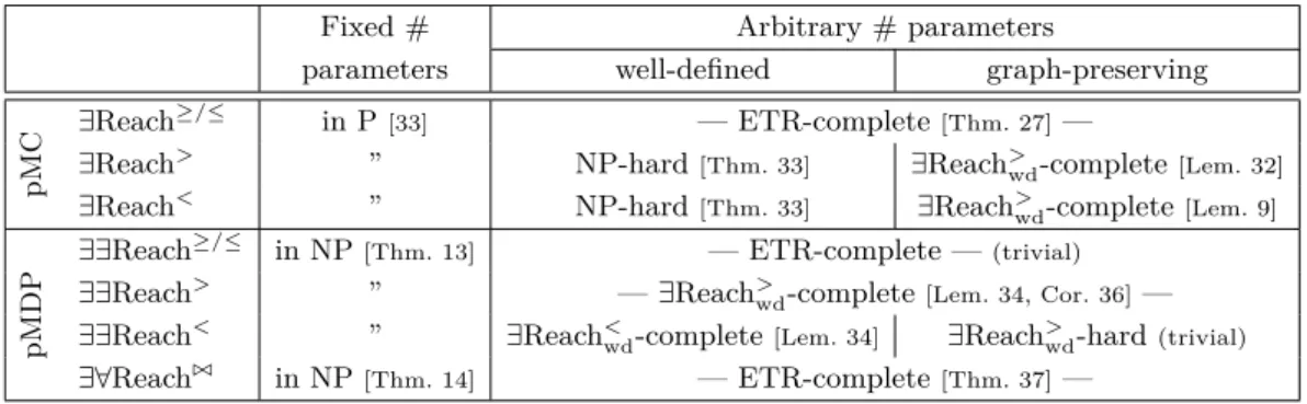
Table 1The complexity landscape for reachability in simple pMDPs. All problems are in ETR.
Fixed # Arbitrary # parameters
parameters well-defined graph-preserving
pMC
∃Reach≥/≤ in P[33] — ETR-complete[Thm. 27]—
∃Reach> ” NP-hard
[Thm. 33] ∃Reach>wd-complete[Lem. 32]
∃Reach< ” NP-hard[Thm. 33] ∃Reach>wd-complete[Lem. 9]
pMDP
∃∃Reach≥/≤ in NP[Thm. 13] — ETR-complete —(trivial)
∃∃Reach> ” —∃Reach>
wd-complete[Lem. 34, Cor. 36]—
∃∃Reach< ” ∃Reach<wd-complete[Lem. 34] ∃Reach>wd-hard(trivial)
∃∀Reach./ in NP[Thm. 14] — ETR-complete[Thm. 37]—
3
Problem landscape
In this section, we introduce the family of decision problems of our main interest. Let a simplepMDPMwith all constants rational, and a setT of target states be the given input. We analyse the decision problems according to whether the setX of parameters fromMhas bounded size – with a-priori fixed bound – or arbitrary size.
It remains for us to fix an encoding for rational functions. Henceforth, we assume the coefficients, exponents and constants are all given as binary-encoded integer pairs.
Decision problems. The first problem is the existence of so-called robust parameter values or lack thereof. More precisely, the question is whether some instantiation ofM is such that its maximal or minimal probability of eventually reachingT compares with 12 in some desired way. In symbols, forQ1,Q2∈ {∃,∀}and./∈ {≤, <, >,≥}, let
Q1Q2Reach./wd def
⇐⇒ Q1val ∈ Pwd,Q2σ∈Σ. PrσM[val](♦T)./
1 2
be the problem of interest. We write Q1Q2Reach./gp whenever Q1 quantifies over
graph-preserving instantiations. We writeQ1Q2Reach./∗ to denote both the wd and gp variants. Furthermore, ifMis a pMC we omit the second quantifier, e.g. ∃Reach<∗. Table 1 surveys the results.
I Proposition 7. For every Q1,Q2 ∈ {∃,∀} and ./ ∈ {≤, <, >,≥}, Q1Q2Reach./∗ are decidable in ETR.
Proof. Both∃∀Reach./∗ and∃∃Reach./∗ are in ETR (for an encoding, see Appendix B in the
technical report). It follows that∃Reach./∗ are also in ETR. J
Problems with fixed threshold. In the above-defined problems, we have fixed a threshold of 12. This is no loss of generality as anygiven rational threshold can be reduced to 12: IRemark 8. An arbitrary threshold 0< λ <1,λ∈Q, is reducible to 12 by the constructions depicted in Fig. 1: If λ≤ 1
2 then we prepend a transition with probabilityp= 2λto the
initial state and with probability 1−pto a sink state. Otherwise, ifλ >12, we prepend a transition with probability q= 2(1−λ) to the initial state and 1−q to the target state. Conversely, the 12 threshold may analogously be reduced to an arbitrary threshold 0< λ <1.
sι 2λ M ⊥ 1−2λ (a)λ≤ 1 2 sι M T 2(1−λ) 1−2(1−λ) PrM(♦T) (b)λ > 12 Figure 1Reductions to reachability thresholdλ=12, cf. Remark 8.
Considerations for the comparison relations.
ILemma 9. For everyQ1,Q2∈ {∃,∀}, there are polynomial-time Karp reductions
among the problemsQ1Q2Reach>gpandQ1Q2Reach<gpand
among the problemsQ1Q2Reach≥gpandQ1Q2Reach≤gp.
The above claim only holds when restricted to graph-preserving parameter spaces.
Semi-continuity. The following theorem formalises an observation in [37, Thm. 5]. ITheorem 10. For each simple pMCM, the function solM is lower semi-continuous, and continuous on PMgp. For acyclic simple pMCs M,solM is continuous on Pwd
M.
Continuity onPMgpfollows assolM is a rational function bounded by [0,1] on all well-defined points [44]. Graph non-preserving instantiations might yield additional sink states in the induced MC, therefore, the probability may drop when changing a parameter instantiation, e.g.p= 0 with an single outgoing transition with probabilitypand a self-loop with probability 1−p.The semi-continuity is the main reason that we do not have symmetric entries for upper and lower bounds in Table 1.
The following result follows immediately from properties of (semi-)continuous functions. I Corollary 11. For all pMDPs, the functions minsolM and maxsolM are lower semi-continuous and have a minimum. For acyclic pMDPs, these functions are semi-continuous.
ICorollary 12. For acyclic pMCs,solM is described by a polynomial even onPwd
M.
4
Fixing the number of parameters
In this section, we assume that the number of parameters is fixed. We focus ourselves on graph-preserving instantiations, as the analysis of pMDPM andPwd
M corresponds to analysing constantly many pMDPsM0 onPgp
M0, cf. Rem. 3.
Upper bounds. Below, we establish NP membership for all variants. ILemma 13. In the fixed parameter case, ∃∃Reach./∗ is in NP.
Proof. Guess a memoryless scheduler. Construct the induced pMC, and verify it in P. J
ITheorem 14. In the fixed parameter case, ∃∀Reach./∗ is in NP.
In the non-parametric case, a schedulerσof an MDP is calledminimalif it minimises Prσ(♦T), i.e. ifσ∈argminσ0∈Σ Prσ
0
(♦T).Consider the probabilitiesxs= Prσ(s→♦T) fors∈S. It is well-known (see, e.g., [43]) thatσis minimal if and only if xs ≤P
s0∈SP(s, a, s0)· xs0 holds for alls∈S anda∈Act(s). (There is a similar condition formaximal schedulers.)
The minimality criterion can be lifted to the parametric case: SupposeR⊆ Pwdis a
graph-consistent region and letfs=solMs σ. Thenσissomewhere minimal onRif and only if there exists someval∈Rsuch that
fs[val]≤ X
s0∈S
P(s, a, s0)·fs0[val] (1)
for alls∈Sanda∈Act. (Foreverywhereminimal strategies, a universal quantification over val yields the correct criterion).
ILemma 15. In the fixed parameter case, checking whether a given strategy is somewhere (resp. everywhere) minimal (resp. maximal) on Pwd is in P.
Proof sketch. Condition (1) can be reformulated as the ETR formula with|X|many variables
Ψ =∃val: ΦR(val)−→Φσ(val) (2)
where ΦR(val) is a formula which is true if and only ifval ∈R and Φσ(val) = ^ s∈S ^ a∈Act gs[val]· Y s06=s hs0[val] ≤ X s0∈S P(s, a, s0)·gs0[val]· Y s006=s0 hs00[val] (3)
wheregs/hs=fs forgs, hs∈Q[val]. (W.l.o.g. it holds that hs[val]>0 for allval ∈R.) J
Proof sketch of Thm. 14. Consider./=≥: Guess a somewhere minimal scheduler. Check
its minimality similar to Lem. 15, but extended to simultaneously ensure that the induced pMC satisfies the threshold. The other relations in./ are analogous. J Sets of optimal schedulers. For the problems∀∀Reach./∗ and∀∃Reach./∗ (with fixed para-meters) we already have coNP-membership (as we considered their complements before). It is tempting to assume that their NP-membership can be established analogous to above, relying oneverywhereoptimal schedulers which, according to Lem. 15, can also be verified in polynomial time. However, such schedulers do not necessarily exist. What we need instead is aset of somewhere optimal schedulers covering the entire parameter space – a so called optimal-scheduler set (OSS).
IDefinition 16 (Optimal scheduler set). A set Ω ⊆Σ is called an optimal scheduler set (OSS) onR⊆ Pwd if
∀val∈R,∃σ∈Ω. PrσM[val](♦T) = max σ0∈ΣPr
σ0
M[val](♦T),
i.e. Ω contains a maximal scheduler for every point in the regionR. The notion can be analogously defined for minimal schedulers.
An OSS of minimal cardinality is called a minimal optimal scheduler set(MOSS). For many applications it is appropriate to describe a regionRvia a quantifier-free ETR-formula ΦR with|X|free variables such thatSat(ΦR) =R. In that case, we have the following: ITheorem 17. In the fixed parameter case, checking whether a given Ω⊆Σconstitutes an OSS onR=Sat(ΦR) can be done in time polynomial in the size ofM,ΩandΦR.
Proof. For everyσ∈Ω, we construct the formulas Φσ as in (3) in polynomial time. Then,
we check whether the fixed-parameter ETR-formula ∃val: ΦR(val)−→
^
σ∈Ω
¬Φσ(val)
Checking whether a set is a MOSS then additionally requires consideration of all the subsets with one element removed (again in polynomial time).
ILemma 18. If the size of a MOSS on Pwd is polynomially bounded for fixed-parameter
pMDPs, then∃∃Reach./∗ and∃∀Reach./∗ are in coNP.
The proof considers the complement of∃∀Reach./∗, that is∀∃Reach./∗¯. Under the assumption in the lemma, it now suffices to guess a MOSS and verify∃Reach./∗¯ on the induced pMCs in polynomial time, showing that the complement is in NP.
In the arbitrary parameter case, we obtain an exponential lower bound on the MOSS size: ILemma 19. There exists a family(Mn)n∈Nof simple pMDPs withn+2states s.t.|Ω| ≥2
n
for any OSSΩonPwd, i.e., the size of a MOSS can grow exponentially in the pMDP’s size.
This lemma, and what follows below, consider the unbounded parameter case, i.e., from now on, parameters are part of the input.
5
The expressiveness of simple pMCs
We investigate the relation between polynomial inequalities and the∃Reach problems. The first lemma in this section is a key ingredient for our complexity analysis later on.
ILemma 20 (Chonev’s trick [16, Remark 7]). Let f ∈ Q[X] be a polynomial, µ ∈Qand 0< λ < 1. There exists a simple acyclic pMC M with a target stateT such that for all val:X →[0,1]and all comparison relations ./∈ {<,≤,≥, >,=}it holds that
f[val]./ µ⇐⇒PrM[val](♦T)./ λ.
Moreover, ifd is the total degree of f, t the number of terms in f and κa bound on the (bit-)size of the coefficients and the thresholds µ, λ, then M can be constructed in time
O(poly(d, t, κ)).
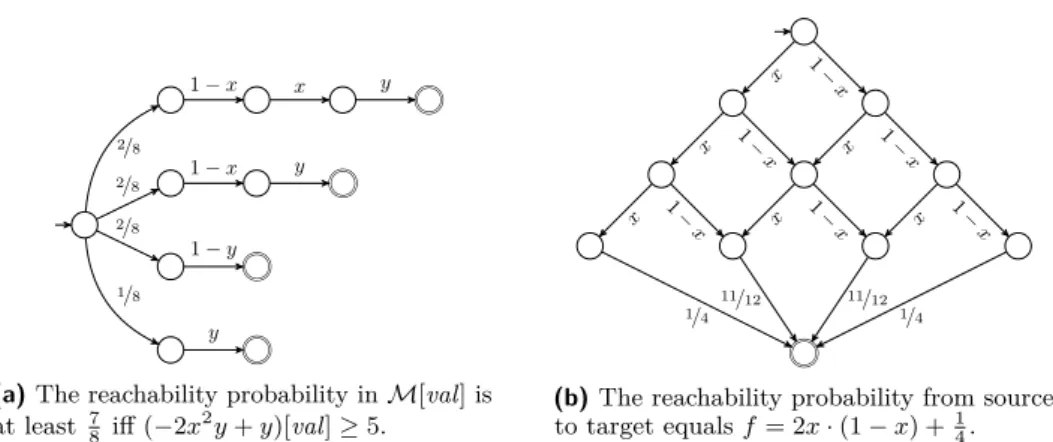
I Example 21. Consider the inequality −2x2y+y
> 5. We reformulate this to: 2 · ((1−x)xy+ (1−x)y+ (1−y)−1)+y>5 and then to 2·(1−x)xy+2·(1−x)y+2·(1−y)+y> 7. Observe that both sides now only contain positive coefficients. Furthermore, observe that we wrote the left-hand side as sum of products over{x,1−x, y,1−y}. After rescaling (with
1
8), we can construct the pMCMdepicted in Fig. 2a and setλ= 7 8.
Checking a bound on a given polynomial overX thus is equivalent to checking a bound on a reachability probability in a simple acyclic pMC overX. For the fixed parameter case, this gives rise to the following equivalence relating arbitrary pMCs to simple acyclic pMCs. ITheorem 22. For any non-simple pMCMwithPMgp= (0,1)Xthere exists a simple acyclic pMCM0 such that
{val ∈ PMgp|PrM[val](♦T)./ λ}={val ∈ P gp
M0 |PrM0[val](♦T)./ λ}. In the fixed parameter case,M0 can be computed in polynomial time.
The proof is constructive: one first computes the (rational function)solM, reformulates that as a polynomial constraint, and casts that into a simple acyclic pMC using Lemma 20.
The goal of the rest of this section is to prove a result which is, in a sense, a stronger version of Lemma 20. In particular, we want to describe polynomials bysolM for an acyclic pMC. We call a polynomialf ∈Q[X]adequateif 0< f[val]<1 for allval:X→(0,1) and 0≤f[val]≤1 for all val:X →[0,1]. Note that solM is an adequate polynomial if M is both simple and acyclic, and there is no acyclic pMCM(with a single parameter) such that
2/8 2/8 2/8 1/8 1−x x y 1−x y 1−y y
(a)The reachability probability inM[val] is at least 78 iff (−2x2y+y)[val]≥5.
x 1−x x 1−x x 1−x x 1−x x 1−x x 1−x 1/4 11/12 11/12 1/4
(b)The reachability probability from source to target equalsf = 2x·(1−x) +14.
Figure 2 Examples for the strong connection between polynomial (inequalities) and pMCs.
Transitions to the sink are not depicted for conciseness.
ITheorem 23. Letf ∈Q[x] be a (univariate) adequate polynomial. There exists a simple acyclic pMCM with a target stateT such that f =solM.
Our construction of a pMC for some adequate polynomial is based on the following result: ILemma 24(Handelman’s theorem [30]). Letβ1≥0, . . . , β`≥0be linear constraints that
define a compact convex polyhedron P⊆Rn with interior. If a polynomial f ∈
R[x1, . . . , xn]
is strictly positive on P, thenf may be written as
f = k X i=1 λihi (4) wherehi=βei,1 1 ·. . .·β ei,`
` for some natural exponents ei,j and real coefficientsλi>0. Form (4) is called aHandelman representation off w.r.t.β1, . . . , β`. The next lemma states
the existence of a specific Handelman representation which we can map to a pMC. ILemma 25. Letf ∈Q[x] be an adequate polynomial. There exists ann≥0 such that
f = n X k=0 pk· n k
·xn−k·(1−x)k with pk ∈[0,1]for all 0≤k≤n (5)
IExample 26. Consider f = 2x·(1−x) + 14 which is strictly positive on [0,1] and already in a Handelman representation. Following the proof of Lem. 25, we find that
f =1 4 0 3 x3+11 12 1 3 x2(1−x) +11 12 2 3 x(1−x)2+1 4 3 3 (1−x)3
The construction (described in the proof of Thm. 23) yields the pMC depicted in Fig. 2b.
6
The complexity of reachability in pMCs
We improve lower bounds for∃Reach problems. The results depend on the comparison type: Nonstrict inequalities. This paragraph is devoted to proving the following theorem: ITheorem 27. ∃Reach≤∗,∃Reach≥∗ are all ETR-complete (even for acyclic pMCs).
sx1 s 0 x1 sx2 s 0 x2 . . . s 0 xn sι 1−x1 x1 1−x2 xn x1 1−x1 x2 1−xn
Figure 3Gadget for the proof of Lemma 32.
IDefinition 28. The decision problem modified-closed-bounded-4-feasibility(mb4FEAS-c) asks: Given a (non-negative) quadric polynomial f, ∃val: X →[0,1] s.t.f[val]≤0? The modified-open-bounded-4-feasibility(mb4FEAS-o) is analogously defined with val ranging over(0,1).
This problem easily reduces to its≥-variant by multiplying f with−1. ILemma 29. The problems mb4FEAS-c and mb4FEAS-o are ETR-hard.
Essentially, one reduces from the existence of common roots of quadratic polynomials lying in a unit ball, which is known to be ETR-complete [47, Lemma 3.9]. The reduction to mb4FEAS follows the reduction2between unconstrained variants (i.e., variants in which the position of the root is not constrained) of the same decision problems [48, Lemma 3.2]. IRemark 30. Observe that there may be exactly one satisfying assignment to mb4FEAS-o/c, which may be irrational. In contrast, if there exists a satisfying assignment forf >0, then there exist infinitely many satisfying (rational) assignments. To the best of our knowledge, the complexity of a variant of mb4FEAS-o/c with strict bounds is open. Therefore, we have no ETR-hardness for∃Reach with strict bounds. In general, conjunctions of strict inequalities are also ETR-complete [48]. We exploit this in the proof of Thm. 37 on page 12.
Proof of Thm. 27. The reduction from mb4FEAS-c to∃Reach≤wd is a straightforward
ap-plication of Lemma 20 with µ = 0 andλ = 12. For ∃Reach≤gp, we reduce from the open variant and notice that as the construction in Lemma 20 preserves all satisfying instantiations val:X →[0,1] it, in particular, also preserves them on the graph-preserving parameter space.
For≥, we apply Lemma 20 on−f. J
The tight complexity class shows that the assumption of simplicity is not a real restriction. Furthermore, a similar construction can be used for (sufficiently large3, linear) subsets of the
parameter space. In particular, methods [18, 44] targeted at a variant of∃Reach considering a so-called-preserving parameter space ([, 1−]k) target an ETR-complete problem.
Strict inequalities. In this paragraph, the main result is: ITheorem 31. ∃Reach>* and∃Reach<* are NP-hard.
The gadget in Fig. 3 ensures that for any graph non-preserving instantiation, the probability to reach the target is 0, while it does not affect reachability probabilities for graph-preserving instantiations. Together with semi-continuity of the solution function, we deduce that assuming graph-preservation is equivalent to not making this assumption:
ILemma 32. There are polynomial-time Karp reductions among ∃Reach>gp and∃Reach>wd.
2 Essentially the polynomialf in mb4FEAS is constructed by taking the sum-of-squares of the quadratic
polynomials, and further operations are adequatly shifting the polynomial.
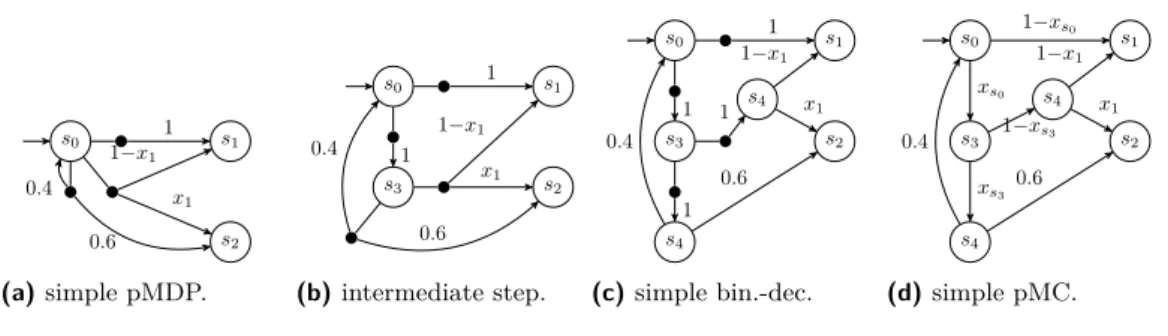
s0 s1 s2 1 1−x1 x1 0.4 0.6 (a)simple pMDP. s0 s1 s2 s3 1−x1 x1 0.4 0.6 1 1 (b)intermediate step. s0 s1 s2 s3 s4 s4 1−x1 x1 0.4 0.6 1 1 1 1 (c)simple bin.-dec. s0 s1 s2 s3 s4 s4 1−x1 x1 0.4 0.6 1−xs3 xs3 1−xs0 xs0 (d)simple pMC.
Figure 4From simple pMDP to simple pMC.
We may thus turn our attention to well-defined parameter spaces: The decision problem ∃Reach≥wd1 ⇐⇒ ∃valdef ∈ Pwd
M. PrM[val](♦T)≥1
is NP-complete [16, Thm. 3]. A more refined analysis of the 3SAT-reduction yields: ITheorem 33. ∃Reach>wd and∃Reach<wd are NP-hard.
Proof of Thm. 31. Lem. 32, Thm. 33, and Lem. 9 together imply Thm. 31. J
This concludes our complexity analysis for pMCs.
7
The complexity of reachability in pMDPs
7.1
Exists-exists reachability
By definition, every pMC is a pMDP. Conversely, from any pMDP we can construct a pMC such that their∃∃Reach./wd problems coincide. A similar construction relates pMCs to the existence of optimal randomised memoryless strategies in partially observable MDPs [37]. ILemma 34. There are polynomial-time Karp reductions among∃Reach./wd and∃∃Reach./wd. We outline the steps in Fig. 4 and in the description below.
Binary-decision pMDPs. The first step of the translation consists in restricting the non-determinism resolved by a scheduler to (at most) two options from every state. A binary-decision pMDP is a pMDP such that|Act(s)| ≤2 for all statess∈Sand if|Act(s)|= 2 then ∀a ∈Act(s),∀s0 ∈S, P(s, a, s0) ∈ {0,1}. Any pMDP can be transformed (in polynomial time) into a binary-decision pMDP by introducing auxiliary states and simulating k-ary non-deterministic choice using a binary-tree-like scheme in which all non-Dirac transitions are pushed to the leaves (see, e.g., [37, 44, 49]). Such a construction preserves simplicity. From non-determinism to parameters. For a given binary-decision pMDP M, we may replace all non-determinism by parameters, inspired by [28, 37]. We introduce fresh variables XS ={xs|s∈S}. InM, for any stateswithAct(s) ={a, a0}we replace
the unique transitionP(s, a, s0) = 1 byP(s, a, s0) =x
s the unique transitionP(s, a0, s0) = 1 byP(s, a0, s0) = 1−xs.
The outcome is a simple pMCM0. To translate instantiations into schedulers, and vice versa, it is helpful to consider randomised schedulers. Observe that, by Rem. 5, instantiations which translate into such schedulers are always dominated by deterministic ones.
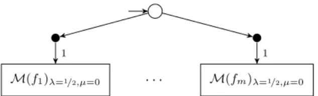
. . .
M(f1)λ=1/2,µ=0 M(fm)λ=1/2,µ=0
1 1
Figure 5Construction for the proof of Thm. 37.
ILemma 35. For all simple pMDPsM one can construct in polynomial time a (linearly larger) simple pMCM0 s.t. ∃val ∈ Pwd M,∃σ∈Σ. Pr σ M[val](♦T)./ 1 2 ⇐⇒ ∃val ∈ Pwd M0. PrM0[val](♦T)./ 1 2 .
ICorollary 36. There are polynomial-time Karp reductions among∃∃Reach>gpand∃Reach>wd.
Proof. Minor adaptions in the proofs of Lemma 34 and Lemma 32. J
7.2
Exists-forall reachability
Contrary to pMCs, we obtain ETR-completeness in pMDPs for any comparison relation: ITheorem 37. ∃∀Reach./∗ are all ETR-complete (even for acyclic pMDPs with a single non-deterministic state).
For the strict relations, we use a different problem to reduce from.
IDefinition 38. The decision problem bounded-conjunction-of-inequalities(bcon4INEQ-c) asks: Given a family of quadric polynomialsf1, . . . , fm,∃val :X →[0,1]s.t.
Vm
i=1fi[val]<0?
The open variant (bcon4INEQ-o) can be defined analogously. By a reduction from mb4FEAS (adapted from [48, Thm 4.1]): ILemma 39. The bcon4INEQ-o/c problems are ETR-hard.
Proof sketch of Thm. 37. ETR-hardness for non-strict inequalities follows from Thm. 27.
For strict inequalities, we reduce from bcon4INEQ-o/c: Generalise the construction from Thm. 27: Build a pMDP as in Fig. 5 with pMCsM(fi)λ=1/2,µ=0 created by Lemma 20. J
Relation to stochastic games
We argue that pMDPs are – in a sense – a generalisation ofConcurrent Stochastic Reachability Games (CSRG), a model which has been extensively studied [11, 12, 20, 31, 52].
Playing a stochastic game. A CSRG is a two-player gameG played on a finite set S of states. The objective of player I is to reach a target states T ⊆S while player II has to avoid ever reaching a state inT. A play of Gbegins in an initial state sι and proceeds as follows: In states, both players I and IIconcurrently select an actiona∈As (resp.b∈Bs), the finite set of actions available to player I (resp. II) in states. The game then picks a successor states0 according to a fixed probability distributionP(·|s, a, b) overS, and the play continues ins0. The transition fromstos0 is called around ofG. Player I wins Gonce a state inT is reached. Otherwise, if a target is never reached, then II wins.
A strategyσof a player is, in essence, a scheduler. However, strategies in a CSRG map state-action sequencess0(a0, b0). . . sk−1(ak−1, bk−1)sk to a probability distribution over the
actionsAsk (resp. Bsk) available in the current statesk. We callσ astationary strategy
if it does not depend on the history but only on the current state, i.e. it is a randomised memoryless scheduler. Let Σi denote the set of stationary strategies for playeri∈ {I,II}.
Instantiations and MDPs. Theinstantiation Gσ ofG with a stationary strategy for player I is the structure obtained by forcing player I to followσ. Notice thatGσ is a finite MDP
M. Its transition probability functionPMis obtained by letting
PM(s, b, s0) =
X
a∈As
σ(a|s)P(s0|s, a, b) (6)
for all s, s0 ∈ S and actions b ∈ B
s of player II. (Instantiations are defined completely symmetrically for strategies of player II.) Conversely, every MDP may be viewed as a CSRG where|As|= 1 (or|Bs|= 1) for alls∈S, i.e. one of the players does never have any choice.
Value of a CSRG. Let Prσ,τG (♦T) be the probability thatT is reached if player I plays accord-ing toσand player II according toτ. ThevalueofGis defined asV(G) := supσinfτPr
σ,τ
G (♦T) where the sup and inf range over all strategies of both players respectively. Intuitively, it is the maximal winning probability of player I that can be guaranteed against all strategies of player II. The existence of stationary optimal strategies for player II [32, 41] allows us to encode a CSRG in a pMDP by replacing the universal player II with parameters:
ITheorem 40. For any given CSRGG, there exists a simple pMDP Msuch that
V(G) = min τ∈ΣIImaxσ∈ΣIPr σ,τ G (♦T) = min val∈Pwdmaxσ∈ΣPr σ M[val](♦T)
andMcan be computed in polynomial time (in the size ofG). As a direct consequence, we obtain CSRG-hardness.
ICorollary 41. Determining whetherV(G)λ, for λ∈Q, reduces to∃∀Reachwd. It follows from [11, Thms. 6 and 12] that optimal rational instantiations may be complex. ITheorem 42. There are pMDPs for which rational optimal andε-optimal parameter values minimising the valuemaxσ∈ΣPrσM[val](♦T)require exponentially-many bits to be written as
a binary-encoded integer-pair.
8
Robust reachability
In this section, we briefly consider pMDPs in which we focus on obtaining (robust) schedulers rather than (robust) parameter values: We swap the quantification order from theQ1Q2Reach
problem. Intuitively, we ask whether some scheduler gives guarantees on the maximal or minimal probability of all instantiations of the pMDP eventually reachingT. Formally, for eachQ1,Q2∈ {∃,∀}and./∈ {≤, <, >,≥}, let
Q1Q2RobReach./wd def
⇐⇒ Q1σ∈Σ, Q2val ∈ Pwd. PrσM[val](♦T)./
1 2.
We adopt the same conventions as for the Q1Q2Reach problem when considering
graph-preserving instantiations. Variants which use the same quantifier twice, or consider pMCs yield the same results as for Reach./, and are therefore omitted.
Robust strategies have been widely studied in the field of operations research (see, e.g., [40, 57]) and are the main focus ofreinforcement learning [55]. It is known that the robust-reachability problem as defined above is not the most general question one can ask. Indeed, we restrict our attention tomemoryless schedulers while, in general, optimal robust schedulers require memory and randomisation [1].
Our interest in the robust-reachability problem is twofold. First, it naturally corresponds to the quantifier-swapped version of the reachability problem. Second, memoryless schedulers are desirable in practice for their comprehensibility and ease of implementation.
ITheorem 43. In the fixed parameter case,∃∀RobReach</>
∗ are NP-complete. NP-hardness holds even for acyclic pMDPs with a single parameter.
Proof sketch. Membership in NP is analogous to Lem. 13. NP-hardness is based on a
reduction from 3-SAT, with a construction similar to Fig. 5. J
IProposition 44. The decision problems∃∀RobReach./∗ are NP-hard and coNP-hard, and in PSPACE. For non-strict inequalities, the problems are coETR-hard.
Proof. NP-hardness follows from Thm. 43, coNP/coETR-hardness follows from Thm. 31,
Thm. 33, and Thm. 27, respectively. Iterating over all (finitely many) schedulers, check each
scheduler in ETR or in coETR (and thus in PSPACE). J
Consequently, it is unlikely that either of the problems are in ETR or coETR, as then ETR and coETR would coincide (which is not impossible, but unlikely [48]).
9
Conclusions
We have studied the complexity of various reachability problems forsimplepMCs and pMDPs. All the problems we have considered are easily seen to be solvable in PSPACE via reductions to the existential theory of the reals. We have complemented this observation with lower bounds, i.e. ETR hardness for several versions of the problem both for (tree-like) pMCs and pMDPs. These lower bounds naturally extend to general pMCs and pMDPs, and to expected reward measures.
We have given an NP decision procedure for pMDPs with a fixed number of parameters. The exact complexity of pMDP reachability problems with this restriction remains open, and our upper bounds do not straightforwardly generalise beyond simple pMDPs (see Rem. 3). Finally, we have established a tight connection between polynomials and pMCs (even beyond [16]). However, our results do not allow us to conclude whether there always are “small” pMCs for every polynomial. Such a result would provide more evidence of ETR being
the right framework to solve problems for our parametric models.
References
1 Sebastian Arming, Ezio Bartocci, and Ana Sokolova. SEA-PARAM: exploring schedulers in parametric MDPs. InQAPL@ETAPS, volume 250 ofEPTCS, pages 25–38, 2017.
2 Christel Baier and Joost-Pieter Katoen.Principles of model checking. MIT Press, 2008. 3 Ezio Bartocci, Radu Grosu, Panagiotis Katsaros, C. R. Ramakrishnan, and Scott A. Smolka.
Model Repair for Probabilistic Systems. InTACAS, volume 6605 ofLNCS, pages 326–340. Springer, 2011.
4 Saugata Basu, Richard Pollack, and Marie-Françoise Roy. Existential theory of the reals.
5 Daniel S. Bernstein, Robert Givan, Neil Immerman, and Shlomo Zilberstein. The Complexity of Decentralized Control of Markov Decision Processes. Math. Oper. Res., 27(4):819–840, 2002. 6 Luca Bortolussi and Simone Silvetti. Bayesian Statistical Parameter Synthesis for Linear
Temporal Properties of Stochastic Models. InTACAS (2), volume 10806 ofLNCS, pages 396–413. Springer, 2018.
7 John F. Canny. Some Algebraic and Geometric Computations in PSPACE. InSTOC, pages 460–467. ACM, 1988.
8 Milan Ceska, Frits Dannenberg, Nicola Paoletti, Marta Kwiatkowska, and Lubos Brim. Precise parameter synthesis for stochastic biochemical systems. Acta Inf., 54(6):589–623, 2017. 9 Krishnendu Chatterjee. Robustness of Structurally Equivalent Concurrent Parity Games. In
FOSSACS, volume 7213 ofLNCS, pages 270–285. Springer, 2012.
10 Krishnendu Chatterjee, Martin Chmelik, and Jessica Davies. A Symbolic SAT-Based Algorithm for Almost-Sure Reachability with Small Strategies in POMDPs. InAAAI, pages 3225–3232. AAAI Press, 2016.
11 Krishnendu Chatterjee, Kristoffer Arnsfelt Hansen, and Rasmus Ibsen-Jensen. Strategy Complexity of Concurrent Safety Games. InMFCS, volume 83 ofLIPIcs, pages 55:1–55:13. Schloss Dagstuhl - Leibniz-Zentrum fuer Informatik, 2017.
12 Krishnendu Chatterjee and Thomas A. Henzinger. A survey of stochastic omega-regular games.
J. Comput. Syst. Sci., 78(2):394–413, 2012.
13 Taolue Chen, Yuan Feng, David S. Rosenblum, and Guoxin Su. Perturbation Analysis in Verification of Discrete-Time Markov Chains. InCONCUR, volume 8704 ofLNCS, pages 218–233. Springer, 2014.
14 Taolue Chen, Ernst Moritz Hahn, Tingting Han, Marta Z. Kwiatkowska, Hongyang Qu, and Lijun Zhang. Model Repair for Markov Decision Processes. InTASE, pages 85–92. IEEE Computer Society, 2013.
15 Taolue Chen, Tingting Han, and Marta Z. Kwiatkowska. On the complexity of model checking interval-valued discrete time Markov chains. Inf. Process. Lett., 113(7):210–216, 2013. 16 Ventsislav Chonev. Reachability in Augmented Interval Markov Chains.CoRR, abs/1701.02996,
2017. arXiv:1701.02996.
17 Anne Condon. Computational models of games. ACM distinguished dissertations. MIT Press, 1989.
18 Murat Cubuktepe, Nils Jansen, Sebastian Junges, Joost-Pieter Katoen, and Ufuk Topcu. Synthesis in pMDPs: A Tale of 1001 Parameters. InATVA, volume 11138 ofLNCS, pages 160–176. Springer, 2018.
19 Conrado Daws. Symbolic and Parametric Model Checking of Discrete-Time Markov Chains. InICTAC, volume 3407 ofLNCS, pages 280–294. Springer, 2004.
20 Luca de Alfaro, Thomas A. Henzinger, and Orna Kupferman. Concurrent reachability games.
Theor. Comput. Sci., 386(3):188–217, 2007.
21 Christian Dehnert, Sebastian Junges, Nils Jansen, Florian Corzilius, Matthias Volk, Harold Bruintjes, Joost-Pieter Katoen, and Erika Ábrahám. PROPhESY: A PRObabilistic ParamEter SYnthesis Tool. InCAV (1), volume 9206 ofLNCS, pages 214–231. Springer, 2015.
22 Christian Dehnert, Sebastian Junges, Joost-Pieter Katoen, and Matthias Volk. A Storm is Coming: A Modern Probabilistic Model Checker. InCAV (2), volume 10427 ofLNCS, pages 592–600. Springer, 2017.
23 Karina Valdivia Delgado, Scott Sanner, and Leliane Nunes de Barros. Efficient solutions to factored MDPs with imprecise transition probabilities. Artif. Intell., 175(9-10):1498–1527, 2011.
24 Antonio Filieri, Giordano Tamburrelli, and Carlo Ghezzi. Supporting Self-Adaptation via Quantitative Verification and Sensitivity Analysis at Run Time. IEEE Trans. Software Eng., 42(1):75–99, 2016.
25 Paul Gainer, Ernst Moritz Hahn, and Sven Schewe. Accelerated Model Checking of Parametric Markov Chains. InATVA, volume 11138 ofLNCS, pages 300–316. Springer, 2018.
26 Sergio Giro, Pedro R. D’Argenio, and Luis María Ferrer Fioriti. Distributed probabilistic input/output automata: Expressiveness, (un)decidability and algorithms. Theor. Comput. Sci., 538:84–102, 2014.
27 Robert Givan, Sonia Leach, and Thomas Dean. Bounded-parameter Markov decision processes.
Artif. Intell., 122(1-2):71–109, 2000.
28 Ernst Moritz Hahn, Tingting Han, and Lijun Zhang. Synthesis for PCTL in Parametric Markov Decision Processes. InNASA Formal Methods, volume 6617 ofLNCS, pages 146–161. Springer, 2011.
29 Ernst Moritz Hahn, Holger Hermanns, and Lijun Zhang. Probabilistic reachability for parametric Markov models. STTT, 13(1):3–19, 2010.
30 David Handelman. Representing polynomials by positive linear functions on compact convex polyhedra. Pacific Journal of Mathematics, 132(1):35–62, 1988.
31 Kristoffer Arnsfelt Hansen, Michal Koucký, and Peter Bro Miltersen. Winning Concurrent Reachability Games Requires Doubly-Exponential Patience. InLICS, pages 332–341. IEEE Computer Society, 2009.
32 CJ Himmelberg, Thiruvenkatachari Parthasarathy, TES Raghavan, and FS Van Vleck. Exist-ence of p-equilibrium and optimal stationary strategies in stochastic games.Proceedings of the American Mathematical Society, 60(1):245–251, 1976.
33 Lisa Hutschenreiter, Christel Baier, and Joachim Klein. Parametric Markov Chains: PCTL Complexity and Fraction-free Gaussian Elimination. InGandALF, volume 256 ofEPTCS, pages 16–30, 2017.
34 Nils Jansen, Florian Corzilius, Matthias Volk, Ralf Wimmer, Erika Ábrahám, Joost-Pieter Katoen, and Bernd Becker. Accelerating Parametric Probabilistic Verification. In QEST, volume 8657 ofLNCS, pages 404–420. Springer, 2014.
35 Bengt Jonsson and Kim Guldstrand Larsen. Specification and Refinement of Probabilistic Processes. InLICS, pages 266–277. IEEE Computer Society, 1991.
36 Sebastian Junges, Erika Abraham, Christian Hensel, Nils Jansen, Joost-Pieter Katoen, Tim Quatmann, and Matthias Volk. Parameter Synthesis for Markov Models. CoRR, abs/1903.07993, 2019. arXiv:1903.07993.
37 Sebastian Junges, Nils Jansen, Ralf Wimmer, Tim Quatmann, Leonore Winterer, Joost-Pieter Katoen, and Bernd Becker. Finite-State Controllers of POMDPs using Parameter Synthesis. InUAI, pages 519–529. AUAI Press, 2018.
38 Marta Z. Kwiatkowska, Gethin Norman, and David Parker. PRISM 4.0: Verification of probabilistic real-time systems. InCAV, volume 6806 ofLNCS, pages 585–591. Springer, 2011. 39 Ruggero Lanotte, Andrea Maggiolo-Schettini, and Angelo Troina. Parametric probabilistic transition systems for system design and analysis. Formal Asp. Comput., 19(1):93–109, 2007. 40 Arnab Nilim and Laurent El Ghaoui. Robust Control of Markov Decision Processes with
Uncertain Transition Matrices. Operations Research, 53(5):780–798, 2005.
41 Thiruvenkatachari Parthasarathy. Discounted and positive stochastic games.Bulletin of the American Mathematical Society, 77(1):134–136, 1971.
42 Alberto Puggelli, Wenchao Li, Alberto L. Sangiovanni-Vincentelli, and Sanjit A. Seshia. Polynomial-Time Verification of PCTL Properties of MDPs with Convex Uncertainties. In
CAV, volume 8044 ofLNCS, pages 527–542. Springer, 2013. 43 Martin L. Puterman.Markov Decision Processes. Wiley, 1995.
44 Tim Quatmann, Christian Dehnert, Nils Jansen, Sebastian Junges, and Joost-Pieter Katoen. Parameter Synthesis for Markov Models: Faster Than Ever. InATVA, volume 9938 ofLNCS, pages 50–67, 2016.
45 James Renegar. On the Computational Complexity and Geometry of the First-Order Theory of the Reals, Part I: Introduction. Preliminaries. The Geometry of Semi-Algebraic Sets. The Decision Problem for the Existential Theory of the Reals. J. Symb. Comput., 13(3):255–300, 1992.
46 Stuart J. Russell and Peter Norvig. Artificial Intelligence - A Modern Approach. Pearson Education, 2010.
47 Marcus Schaefer. Realizability of Graphs and Linkages, pages 461–482. Springer New York, 2013.
48 Marcus Schaefer and Daniel Stefankovic. Fixed Points, Nash Equilibria, and the Existential Theory of the Reals. Theory Comput. Syst., 60(2):172–193, 2017.
49 Roberto Segala and Andrea Turrini. Comparative Analysis of Bisimulation Relations on Alternating and Non-Alternating Probabilistic Models. InQEST, pages 44–53. IEEE Computer Society, 2005.
50 Koushik Sen, Mahesh Viswanathan, and Gul Agha. Model-Checking Markov Chains in the Presence of Uncertainties. InTACAS, volume 3920 ofLNCS, pages 394–410. Springer, 2006. 51 Sven Seuken and Shlomo Zilberstein. Formal models and algorithms for decentralized decision making under uncertainty. Autonomous Agents and Multi-Agent Systems, 17(2):190–250, 2008. 52 Lloyd S. Shapley. Stochastic Games. PNAS, 39(10):1095–1100, 1953.
53 Eilon Solan. Continuity of the value of competitive Markov decision processes. Journal of Theoretical Probability, 16(4):831–845, 2003.
54 Jeremy Sproston. Qualitative Reachability for Open Interval Markov Chains. InRP, volume 11123 ofLNCS, pages 146–160. Springer, 2018.
55 Richard S. Sutton and Andrew G. Barto. Reinforcement learning - an introduction. Adaptive computation and machine learning. MIT Press, 1998.
56 Nikos Vlassis, Michael L. Littman, and David Barber. On the Computational Complexity of Stochastic Controller Optimization in POMDPs. TOCT, 4(4):12:1–12:8, 2012.
57 Wolfram Wiesemann, Daniel Kuhn, and Berç Rustem. Robust Markov Decision Processes.
Math. Oper. Res., 38(1):153–183, 2013.
58 Di Wu and Xenofon D. Koutsoukos. Reachability analysis of uncertain systems using bounded-parameter Markov decision processes. Artif. Intell., 172(8-9):945–954, 2008.