Elsevier Editorial System(tm) for Expert Systems With Applications
Manuscript Draft Manuscript Number: ESWA-D-16-03702R1
Title: Efficient Heuristics for the Parallel Blocking Flow Shop Scheduling Problem
Article Type: Full length article
Keywords: Parallel flow shop; distributed permutation flow shop; blocking flow shop; scheduling
Corresponding Author: Professor Imma Ribas, Ph.D
Corresponding Author's Institution: Universitat Politecnica de Catalunya First Author: Imma Ribas, Ph.D
Order of Authors: Imma Ribas, Ph.D; Ramon Companys, PhD; Xavier Tort-Martorell, PhD
Efficient Heuristics for the Parallel Blocking Flow Shop
Scheduling Problem
Imma Ribas
1,a, Ramon Companys
b, Xavier Tort-Martorell
ca, Departament d’Organització d’Empreses, DOE – ETSEIB - Universitat Politècnica de Catalunya. BarcelonaTech, Avda. Diagonal, 647, 7th Floor, 08028 Barcelona, Spain. E-mail: [email protected] b, CDE - EPSEB - Universitat Politècnica de Catalunya. BarcelonaTech, Gregorio Marañón 44-50, 3rd
Floor, 08028 Barcelona, Spain. E-mail: [email protected]
c, Departament de Estadística e investigación Operativa- ETSEIB - Universitat Politècnica de Catalunya. BarcelonaTech, Avda. Diagonal, 647, 6th Floor, 08028 Barcelona, Spain. E-mail: [email protected]
Abstract
We consider the NP-hard problem of scheduling n jobs in F identical parallel flow shops, each consisting of a series of m machines, and doing so with a blocking constraint. The applied criterion is to minimize the makespan, i.e., the maximum completion time of all the jobs in F flow shops (lines). The Parallel Flow Shop Scheduling Problem (PFSP) is conceptually similar to another problem known in the literature as the Distributed Permutation Flow Shop Scheduling Problem (DPFSP), which allows modeling the scheduling process in companies with more than one factory, each factory with a flow shop configuration. Therefore, the proposed methods can solve the scheduling problem under the blocking constraint in both situations, which, to the best of our knowledge, has not been studied previously. In this paper, we propose a mathematical model along with some constructive and improvement heuristics to solve the parallel blocking flow shop problem (PBFSP) and thus minimize the maximum completion time among lines. The proposed constructive procedures use two approaches that are totally different from those proposed in the literature. These methods are used as initial solution procedures of an iterated local search (ILS) and an iterated greedy algorithm (IGA), both of which are combined with a variable neighborhood search (VNS). The proposed constructive procedure and the improved methods take into account the characteristics of the problem. The computational evaluation demonstrates that both of them –especially the IGA– perform considerably better than those algorithms adapted from the DPFSP literature.
Keywords:
Parallel flow shop,
distributed permutation flow shop; blocking flow shop; scheduling
1 Corresponding author.
E-mail address: [email protected]
Highlights
New Constructive heuristic for both the PBFSP and the DBFSP Combination of IGA and ILS methods with two types of VNS A MILP model solved for small-sized instances
The proposed methods are very effective
Efficient Heuristics for the Parallel Blocking Flow Shop
Scheduling Problem
Imma Ribas
1,a, Ramon Companys
b, Xavier Tort-Martorell
ca, Departament d’Organització d’Empreses, DOE – ETSEIB - Universitat Politècnica de Catalunya. BarcelonaTech, Avda. Diagonal, 647, 7th Floor, 08028 Barcelona, Spain. E-mail: [email protected] b, CDE - EPSEB - Universitat Politècnica de Catalunya. BarcelonaTech, Gregorio Marañón 44-50, 3rd
Floor, 08028 Barcelona, Spain. E-mail: [email protected]
c, Departament de Estadística e investigación Operativa- ETSEIB - Universitat Politècnica de Catalunya. BarcelonaTech, Avda. Diagonal, 647, 6th Floor, 08028 Barcelona, Spain. E-mail: [email protected]
Abstract
We consider the NP-hard problem of scheduling n jobs in F identical parallel flow shops, each consisting of a series of m machines, and doing so with a blocking constraint. The applied criterion is to minimize the makespan, i.e., the maximum completion time of all the jobs in F flow shops (lines). The Parallel Flow Shop Scheduling Problem (PFSP) is conceptually similar to another problem known in the literature as the Distributed Permutation Flow Shop Scheduling Problem (DPFSP), which allows modeling the scheduling process in companies with more than one factory, each factory with a flow shop configuration. Therefore, the proposed methods can solve the scheduling problem under the blocking constraint in both situations, which, to the best of our knowledge, has not been studied previously. In this paper, we propose a mathematical model along with some constructive and improvement heuristics to solve the parallel blocking flow shop problem (PBFSP) and thus minimize the maximum completion time among lines. The proposed constructive procedures use two approaches that are totally different from those proposed in the literature. These methods are used as initial solution procedures of an iterated local search (ILS) and an iterated greedy algorithm (IGA), both of which are combined with a variable neighborhood search (VNS). The proposed constructive procedure and the improved methods take into account the characteristics of the problem. The computational evaluation demonstrates that both of them –especially the IGA– perform considerably better than those algorithms adapted from the DPFSP literature.
Keywords:
Parallel flow shop,
distributed permutation flow shop; blocking flow shop; scheduling
1 Corresponding author.
E-mail address: [email protected]
Manuscript
1
Introduction
The parallel flow shop scheduling problem can be decomposed into two subproblems: first, assigning each job to one of the F flow shops; then, scheduling the jobs in each flow shop in order to minimize the maximum completion time of jobs, i.e., the global makespan. This problem was studied by He, Kusiak and Artiba (1996) for the purpose of applying it in the glass industry. The manufacturing environment under consideration was an F parallel flow shop with two machines in each. They proposed using mixed integer programming and an efficient heuristic to deal with the problem. Vairaktarakis and Elhafs (2000) analyzed the deterioration in the makespan performance when the two-machine hybrid flow shop problem is assimilated with a parallel two-machine flow shop problem. They concluded that the deterioration of the makespan performance was less than 3%, which, in the case studied, justified the design of a parallel flow shop (i.e., independent manufacturing cells) instead of a hybrid flow shop configuration, as the former is easier to manage. They proposed a O(nP3)-time dynamic programming algorithm for optimally solving 2 flow shops in parallel with two machines. (Cao & Chen, 2010) developed a mathematical model and a Tabu Search algorithm for the PFSP with two machines. Al-Salem (2004) proposed a polynomial-time algorithm to minimize the makespan in two-machine parallel flow shops with proportional processing time. Zhang and Van De Velde (2012) developed approximation algorithms with worst-case performance guarantees for scheduling jobs in 2 and 3 flow shops that are in parallel with 2 machines. Notice that these papers only consider flow shops with two machines, which is the simplest case.
However, the PFSP is conceptually similar to another problem that is known in the literature as the Distributed Permutation Flow Shop Scheduling Problem (DPFSP), which considers a multi-factory production network with a flow shop configuration in each factory. In this environment, the scheduling problem deals with the allocation of jobs to factories and the scheduling of jobs in each plant. The DPFSP was first presented by Naderi & Ruiz (2010). After this publication, several authors proposed various heuristics to solve this problem ((Fernandez-Viagas & Framinan, 2014; Gao & Chen, 2012; Gao, Chen, & Deng, 2013; Gao, Chen, Deng, & Liu, 2012; Gao, Chen, & Liu, 2012; Lin, Ying, & Huang, 2013; Liu & Gao, 2010; Bahman Naderi & Ruiz, 2014; Wang, Wang, Liu, & Xu, 2013; Xu, Wang, Wang, & Liu, 2013)). In these papers, the number of machines in each plant (i.e., each flow shop) is not limited. Therefore, the methods proposed can be used to solve the PFSP with more than two machines in each flow shop. However, neither in the literature about the PFSP nor in that about the DPFSP is the blocking constraint considered.
The blocking flow shop scheduling problem allows many production systems to be modeled when there are no buffers between consecutive machines. In general, it is useful for those
two consecutive stations at pre-established times. Some industrial examples can be found in the iron and steel industry (Gong, Tang, & Duin, 2010); in the treatment of industrial waste and the manufacture of metallic parts (Martinez, Dauzère-Pérès, Guéret, Mati, & Sauer, 2006); and in the use of robotic cells, where a job may block a machine while waiting for the robot to pick it up and move it to the next stage (Sethi, Sriskandarajah, Sorger, Blazewicz, & Kubiak, 1992). The blocking constraint tends to increase the completion time of jobs, because the processed job cannot leave the machine if the next machine is busy. Therefore, the heuristics designed to schedule jobs in this environment have to consider this fact in order to minimize the idle time of machines due to possible blockage. The Parallel Blocking Flow Shop Problem (PBFSP) and the Distributed Blocking Flow Shop Scheduling Problem (DBFSP) deal with the allocation and scheduling of jobs in parallel flow shops and in a multi-factory production network with the blocking constraint included in the manufacturing system. It is interesting to study these problems in order to design specific procedures for them, since other procedures that have been adapted from PFSP and DPFSP probably perform worse as a result of not having been designed to minimize the blocking conditions.
In this paper, we propose new constructive procedures that are built using two different approaches, and some improvement heuristics to solve these problems. The computational evaluation shows not only the good performance of the presented improvement heuristics –in particular the iterated greedy algorithm (IGA) combined with a variable neighborhood search (VNS)– but also the effectiveness of the proposed constructive procedures that help the heuristics achieve good solutions.
2
Problem definition
The problem is defined as follows: n jobs have to be scheduled in one of the F identical flow shops with m machines. Each flow shop (factory) is able to process all jobs. The jobs assigned to a flow shop have to be processed by all machines in the same order, from machine 1 to machine
m. Each job i, i ϵ {1,2,. . .,n} requires a fixed non-negative processing time pj,ion every machine
j, j ϵ {1,2,. . .,m}, which does not change from line to line. Setup times are considered to be included in the processing time. The objective is to schedule the jobs to the different flow shops such that the maximum makespan (Cmax) among them is minimized. We denote σf as the sequence of the nf jobs assigned to flow shop f, and fmax as the flow shop with the maximum makespan. Therefore, a solution is formed by the sequence of jobs in each flow shop (=( σ1, σ2, …, σf)).
Next, we introduce additional notation in order to define the mathematical program associated with this problem: let cj,k,f be the departure time of a job that occupies position k in machine j at flow shop f, and let Cmax be the maximum completion time of the last job processed in any of the
parallel flow shops. Notice that, with the blocking constraint, a job cannot leave the machine until the next machine is free, even if it has finished its operation.
Therefore, according to this notation, the mathematical program can be formalized as follows: max C Min (1) n i x F f n k f i k 1 1,2, 1 1 , ,
(2)
n k F f x n i f i k 1 1,2, 1,2, 1 , ,
(3)
F f n k p x c c n i i f i k f k f k 1,2,. 1,2, 1 , 1 , , , 1 , 1 , , 1
(4)
F f n k m j p x c c n i i j f i k f k j f k j 2,3,, 2,3,. 1,2, 1 , , , , , 1 , ,
(5)
F f n k m j c cj,k,f j1,k1,f 2,3,, 1 2,3,. 1,2,(6)
F f m j cj,0,f 0 1,2, 1,2,,(7)
F f n k c0,k,f 0 1,2,, 1,2,(8)
F f c Cmax m,n,f 1,2,,(9)
k n i n f F xk,i,f 0,1 1,2,, 1,2, 1,2,(10)
F f n i n k cj,k,f 0 1,2,, 1,2, 1,2,(11)
The decision variables are the binary variables xk,i,f ,which take value 1 if job i occupies position k in the sequence of flow shop f. Other variables are the continuous variable cj,k,f and
Cmax .
The objective function is set in equation (1). Constraint set (2) ensures that every job must be exactly at one position and only at one factory. Constraint set (3) ensures that only one job at most can be allocated to each position at a factory. Constraint set (4) defines the departure time of the job which occupies position k in the first machine at factory f. Constraint set (5) specifies the relationship between the departure times of each job in two successive machines at the assigned factory. Constraint set (6) calculates the departure time of a job under the blocking conditions by considering that the next machine has to be available. Constraint sets (7) and (8) are the initial conditions. Constraint set (9) defines the makespan. Finally, constraint sets (10) and (11) define the domain of the decision variables.
3
Constructive Heuristics
As stated before, both the PBFSP and the DBFSP need to deal with two related decisions: the allocation of jobs to flow shops (factories) and the sequence of jobs assigned to each line (plant). To the best of our knowledge, no paper has been published regarding these problems, but some ideas can be taken from the DPFSP literature, particularly the constructive heuristics proposed in Naderi & Ruiz (2010), which consist of jobs being sequenced according to an ordering rule before they are assigned to a facility in accordance with an allocation rule. In this paper, we propose a new method for allocating and sequencing the jobs as well as three new procedures, each of which uses a different approach for solving the problem.
The new allocation method consists of dividing the job sequences into F fractions by assigning a similar load (ΣPi/F) to each flow shop (line). Then, the sequence of jobs assigned to each line is improved by an insertion procedure similar to that used in the second step of NEH (Nawaz, Enscore Jr, & Ham, 1983).
This allocation method has been combined with the following ten sequencing rules. Some of them are used in the Permutation Flow Shop Scheduling Problem (PFSP) and some others were specially designed for the Blocking Flow Shop Scheduling Problem: Shortest Processing Time (SPT), Largest Processing Time (LPT), Johnson’s rule (Johnson, 1954), Palmer’s heuristic (Palmer, 1965), CDS (Campbell, Dudek, & Smith, 1970), NEH (Nawaz et al., 1983), Trapeziums (TR) (Companys, 1966), PF (McCormick, Pinedo, Shenker, & Wolf, 1989), PW (Pan & Wang, 2012) and HPF2 (Ribas & Companys, 2015). The resulting heuristics are named as the sequencing rule plus the number 3, following the notation used in (Naderi & Ruiz, 2010). Therefore, these heuristics are named SPT3, LPT3, Johnson3, Palmer3, CDS3, NEH3, TR3, PF3, PW3 and HPF23.
In the TR rule, two indexes are calculated for each job (S1i and S2i), according to (12) and (13), respectively. Next, jobs are scheduled by applying the Johnson algorithm considering S1i as the processing time of job i in the first machine and S2i as the processing time of i in the second machine.
m j i j i m j p S 1 , ) 1 ( 1 (12)
m j i j i j p S 1 , ) 1 ( 2 (13)It is worth noting that ordering jobs in increasing order of S3i=S1i-S2i obtains the sequence given by Palmer’s heuristic.
The HPF2 procedure is divided into two steps. The first step selects a job to be the first job in the sequence, which minimizes the bicriteria index R(i) according to equation (14).
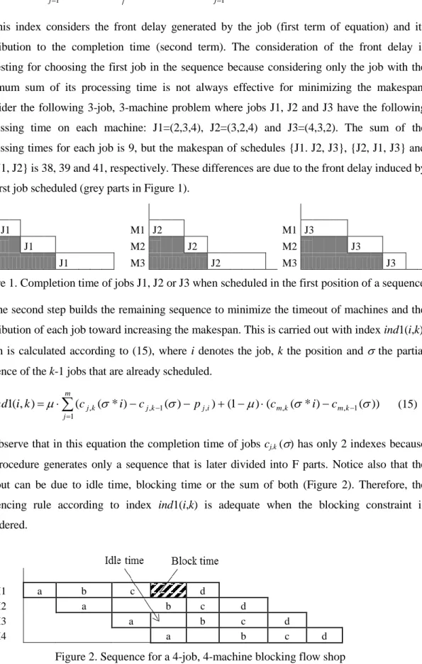
m j i j m j i j m p p j m i R 1 , 1 , ( 1) (1 ) ) ( 2 ) ( (14)This index considers the front delay generated by the job (first term of equation) and its contribution to the completion time (second term). The consideration of the front delay is interesting for choosing the first job in the sequence because considering only the job with the minimum sum of its processing time is not always effective for minimizing the makespan. Consider the following 3-job, 3-machine problem where jobs J1, J2 and J3 have the following processing time on each machine: J1=(2,3,4), J2=(3,2,4) and J3=(4,3,2). The sum of the processing times for each job is 9, but the makespan of schedules {J1. J2, J3}, {J2, J1, J3} and {J3, J1, J2} is 38, 39 and 41, respectively. These differences are due to the front delay induced by the first job scheduled (grey parts in Figure 1).
M1 J1 M1 J2 M1 J3 M2 J1 M2 J2 M2 J3 M3 J1 M3 J2 M3 J3 Figure 1. Completion time of jobs J1, J2 or J3 when scheduled in the first position of a sequence
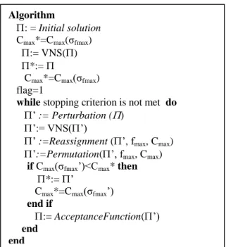
The second step builds the remaining sequence to minimize the timeout of machines and the contribution of each job toward increasing the makespan. This is carried out with index ind1(i,k), which is calculated according to (15), where i denotes the job, k the position and the partial sequence of the k-1 jobs that are already scheduled.
)) ( ) * ( ( ) 1 ( ) ) ( ) * ( ( ) , ( 1 , 1 , , , 1 1 ,
m jk ji mk mk j k j i c p c i c c k i ind (15)Observe that in this equation the completion time of jobs cj,k() has only 2 indexes because the procedure generates only a sequence that is later divided into F parts. Notice also that the timeout can be due to idle time, blocking time or the sum of both (Figure 2). Therefore, the sequencing rule according to index ind1(i,k) is adequate when the blocking constraint is considered. M1 a b c d M2 a b c d M3 a b c d M4 a b c d
Hence, HPF2 can be described as follows:
Step 1: Select the job with minimum R(i), calculated as in (14), and put it in the first position in sequence σ. Set k=1.
Step 2: While k<n, calculate index ind1(i,k) according to equation (15) for each unscheduled job i. Select the job with minimum ind1(i,k). In case of ties, select the job which leads to the partial sequence with minimum makespan. k=k+1.
The new procedures designed specifically for this problem consider both the jobs and lines together. According to this philosophy, we have implemented three methods, which are named RC1_1, RC1_m and RC2.
The RC1_1 and RC1_m procedures are also divided into two steps: the selection of the first job of each line and the building of the remaining sequence according to
i
nd2(i,k,f), calculated as (16), where f is the sequence of jobs already sequenced in line f.
m j i j i j f f k j f m j f k j i c p p c f k i ind 1 , , , , 1 , 1 , ( * ) ( ) ) (1 ) ( ) , , ( 2 (16)In this case, the line is first selected in step 2 in order to proceed with the other jobs. In RC1_1, the line selected is the one which has the first machine available earlier, whereas the line selected in RC1_m is the one which has the last machine available sooner.
RC1_1 and RC1_m can be described as follows:
Step 1: For w=1 to F, select the job with minimum R(i) and put it in the first position in sequence σf. Set k=F.
Step 2:
o (RC1_1): While k<n, select the line f which has the first machine available earlier. Calculate index ind2(i,k,f), as in equation (16), for each unscheduled job
i. Select the job with minimum ind2(i,k,f). In case of ties, select the job which leads to the partial sequence with minimum makespan. k=k+1
o (RC1_m): While k<n, select the line f which has the last machine available sooner. Calculate index ind2(i,k,f) as in equation (16) for each unscheduled job i. Select the job with minimum ind2(i,k,f). In case of ties, select the job which leads to the partial sequence with minimum makespan. k=k+1.
Observe that ind2(i,k,f) weights the timeout with the workload of each job. Therefore, once the line is selected, choosing a job that minimizes this index is adequate for minimizing the makespan under the blocking constraint.
In RC2, the first job assigned to each line is also selected with index R(i); but, to build the remaining sequence, the job and line are selected at the same time in order to minimize index
) ) * ( ( ) 1 ( ) ) ( ) * ( ( ) , , ( 3 , , , , , 0 1 , 1 , i c p c i c c f k i ind f jk f f ji mk f f m j f k j
(17)where f is one of the lines, f is the sequence of jobs already sequenced in line f and c0 is the current minimum makespan of any line.
Therefore, the RC2 procedure can be described as follows:
Step 1: For w=1 to F, select the job with minimum R(i) and put it in the first position in sequence σf. Set k=F.
Step 2: While k<n, select each unscheduled job one by one and calculate ind3(i,k,f)
for
each line, as in equation (17). Select the job and the line that leads to minimumind3(i,k,f). In case of ties, select the job and line which leads to the partial sequence with
minimum makespan.k=k+1.
Observe that ind3(i,k,f) weights the timeout and the difference between the partial makespan (completion time obtained with the jobs already sequenced in this line) as well as the minimum partial makespan obtained in any of the lines. By trying to minimize the second term, the workload of the lines tends to be similar, which is adequate for minimizing the maximum makespan among lines.
The third step in RC1_1, RC1_m and RC2 tries to improve the sequence of each line by using an insertion procedure similar to the one used in heuristic NEH.
Notice that HPF2, RC1_1, RC1_m and RC2 have two parameters (λ and µ) that must be determined adequately. Their calibration is addressed in Section 5.
4
Improvement Heuristics
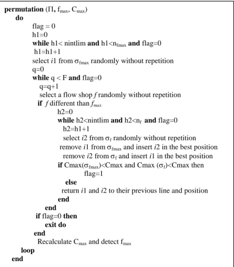
Two simple but effective heuristics for dealing with this problem are presented: an iterated local search algorithm (ILS) and an iterated greedy algorithm (IGA). Both algorithms have a similar scheme. They start with an initial solution, which is improved by applying to the sequence of each line a variable neighborhood search (VNS) based on swap and insert neighborhood structures –named LS1 and LS2, respectively– then, their order is randomly chosen. Next, the solution goes into the main part of the algorithm in order to iteratively apply three procedures that consist of: a Perturbation Mechanism, which modifies the current solution σ and leads to an intermediate solution σ’; an Improvement phase, which tries to improve the current solution by using two neighborhood structures based on the insert and swap movements of jobs between lines (Reassignment and Permutation functions, respectively); and, finally, an
Acceptance function, which chooses the solution to which the next perturbation is applied. The
In the following sections, we explain the different parts of these algorithms, whose main differences are found in the Perturbation Mechanism. The perturbation of IGA is more elaborated than the one used in the ILS, as we will explain later.
Figure 3. Outline of the ILS and IGA algorithm
4.1 Description of the VNS Procedure
The VNS uses two local searches sequentially (named LS1 and LS2),which explore the swap and insert neighborhoods of the current sequence at each flow shop (factory). The neighborhood to be explored first is selected randomly. After exploring the neighboring solutions of current solution σf, the local optimum σf ′ is compared with σf. If the solution has improved, σf′ replaces
σf and the search continues in the other neighborhoods. This process continues until the current solution is no longer improved. Next, the local optimum σf′ is compared with the best solution
σf * in terms of the quality of the solution. If Cmax(σf′) is less than Cmax(σf *), σf′ replaces σf *.
The LS1 procedure is described as follows. For each job in the sequence, neighbors are
generated by swapping a job with all jobs that follow it in the sequence. If the best neighbor (σf′) is better than the current solution (σf), it becomes the new current solution σf, and the process continues until all jobs have been considered. To prevent the neighborhoods from always being explored in the same order, the jobs are selected randomly.
In contrast, LS2 functions as follows. For each job in the sequence, neighbors are generated by removing the job from its position and inserting it into all other possible positions. If the best neighbor (σf ′) is better than the current solution (σf), it becomes the new current solution σf,and the process continues until all jobs have been considered. As in LS1, jobs are selected randomly.
Algorithm
: = Initial solution Cmax*=Cmax(σfmax)
:= VNS() *:=
Cmax*=Cmax(σfmax)
flag=1
while stopping criterion is not met do
’ := Perturbation ()
’:= VNS(’)
’ :=Reassignment (’, fmax, Cmax)
’:=Permutation(’, fmax, Cmax)
if Cmax(σfmax’)<Cmax* then
*:= ’
Cmax*=Cmax(σfmax’)
end if
:= AcceptanceFunction(’)
end end
4.2 Perturbation Mechanism
The implemented Perturbation Mechanism randomly selects a job from one factory and inserts it into the best position of another plant that has been randomly selected. This procedure is repeated d times. Figure 4 shows the outline of the procedure.
Figure 4. Outline of the perturbation mechanism
The perturbation mechanism of IGA goes deeper than the one used in ILS, since it tries to assign each job removed from its line to all the other lines in order to find the factory and position that leads to the minimum makespan among lines. The outline of this procedure can be seen in Figure 5.
Figure 5. Perturbation mechanism of IGA
4.3 Improvement Phase
The Improvement Phase is a variable local search between lines (factories) based on two
neighborhood structures that insert and swap movements of jobs between lines. They are referred to here, respectively, as reassignment and permutation.
Perturbation Mechanism_ILS()
for h=1 tod
Select a job i randomly without repetition fold:= flow shop of job i
fnew:= flow shop selected randomly
Remove job i from fold
Test job i in any possible position σfnew and place it
in the position that leads to the lowest Cmax(σfnew)
nexth
end
Perturbation Mechanism_IG ()
Select d jobs randomly without repetition and put them in sequence Remove the d jobs from their flow shop
for k=1 to d
i:= job of position k in C0=infinite
forf=1 to F
insert i in the best position of f calculate Cmax(f) if Cmax(f)<C0 then C0= Cmax(f) f’=f end nextf f=f’ nextk Calculate Cmax end
The permutation procedure consists of selecting a job randomly from the plant which has the maximum makespan (fmax) and then inserting it into the best position of another randomly selected plant, i.e., the position that leads to a minimum makespan of this line. If the Cmax diminishes, the sequence is kept and the procedure is repeated again with the line that now has the maximum makespan. If the movement does not improve the Cmax, a new job from fmax is selected and the process begins again. This part finishes either when all jobs in the critical line have been selected or after a limited number of iterations (nlimit) are reached. The outline of this procedure is shown in Figure 6.
Figure 6. Outline of permutation procedure.
permutation (, fmax, Cmax)
do
flag= 0 h1=0
while h1< nintlim and h1<nfmax and flag=0
h1=h1+1
select i1 from fmax randomly without repetition
q=0
while q < F and flag=0
q=q+1
select a flow shop f randomly without repetition if f different than fmax
h2=0
while h2<nintlim and h2<nf and flag=0
h2=h1+1
select i2 from f randomly without repetition remove i1 from fmax and insert i2 in the best position
remove i2 from f and insert i1 in the best position
if Cmax(fmax)<Cmax and Cmax (f)<Cmax then
flag=1
else
return i1 and i2 to their previous line and position end
end if flag=0 then exit do end
Recalculate Cmax and detect fmax
loop
The reassignment procedure consists of swapping two jobs: one from fmax and another from another randomly selected line. If the maximum makespan among lines (Cmax) diminishes, the change is kept and the procedure is repeated with the line that now has the maximum makespan. In the same way as the permutation procedure, if the movement does not improve the Cmax, a new job from fmax is selected and the process begins again. The search finishes either when all jobs in the critical line have been selected or after a limited number of iterations (nlimit) are reached. Then the process iterates over each neighborhood to find improvements. The outline of this procedure is shown in Figure 7.
Figure 7. Outline of the reassignment procedure
4.4 Acceptance Function
The Acceptance Function uses a criterion that is similar to the one used in the simulated annealing algorithm. In this case, we use a scheme that is similar to the one used in (Fernandez-Viagas & Framinan, 2014).
5
Experimental Evaluation
In this section, we show the computational evaluation of the constructive procedures and the heuristics methods presented.
The first step was to calibrate and evaluate the constructive procedure in order to select the
reassignment (, fmax, Cmax)
do
flag= 0 h=0
while h< nintlim and h<nfmax and flag=0
h=h+1
select i from fmax randomly without repetition
q=0
while q < F and flag=0
q=q+1
select a line f randomly without repetition if f different than fmax
insert i in the bestposition of f obtaining f’
if Cmax(f’) < Cmax then
flag=1 end end if flag=0 then exit do end
Modify by changing f for f’ and removing i from fmax
Recalculate Cmax and detect fmax
loop
the selected procedures. We then analyzed the general performance of the heuristics by using a set of small-sized instances in which most of the optimal solutions had been found by the proposed mathematical model. Then, finally, we compared them with other adapted heuristics proposed for the DPFSP.
5.1
Calibration of Constructive Procedures
As stated before, HPF2, RC1_1, RC1_m and RC2 have two parameters that must be calibrated. Parameters λ and µ of each heuristic were selected by measuring the performance of the algorithm, which itself was done by combining several λ and µ values. The values of λ and µ
ranged from 0 to 1 in increments of 0.05. Therefore, we tested 21 values for each parameter.
For this test, we used 600 generated instances. 100 instances were grouped into 20 sets of size
n x m (5 instances per set), where n= {25, 50, 100, 200, 400} and m = {5, 10, 15, 20}. All these 100 instances were considered with a different number of factories. We had F={2,3,4,5,6,7}, which gave us 600 instances in total.
The performance was measured by the Relative Percentage Deviation (RPD) from the best solution (minimum makespan), which was obtained during the experiment using all combinations of values. Therefore, RPD is calculated as in (18):
max , 100 k k k h Best Best C RPD (18)
where Cmaxh,k is the makespan obtained in instance k by heuristic h, which is the heuristic that results from combining given values of λ and µ; and Bestk is the minimum Cmax obtained in this instance by any combination of values.
For each procedure, we conducted an Analysis of Variance by including the following terms in the model: F, μ, λ, and their interactions F*μ, F*λ and μ* λ. This allowed us to check the effects of the two parameters while also seeing via their interactions with F whether or not their best values were dependent on the number of factories. The result from the four cases indicated a dominating, very strong and highly significant effect of μ and significant but very weak effects
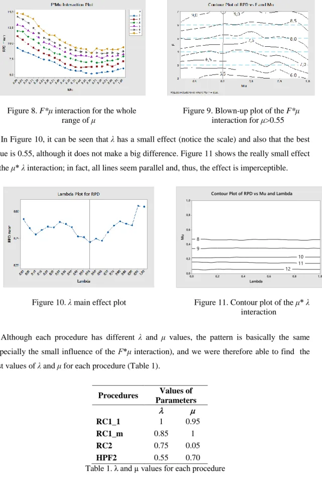
of , λ, F*μ and μ* λ. As an example, Figure 8 shows the F*μ interaction for the whole range of
μ. The dominating effect of μ is clear. To find the best μ value (0.7 in this case), a blown-up plot of the best region was produced (Figure 9).
Figure 8. F*μ interaction for the whole range of μ
Figure 9. Blown-up plot of the F*μ
interaction for μ>0.55
In Figure 10, it can be seen that λ has a small effect (notice the scale) and also that the best value is 0.55, although it does not make a big difference. Figure 11 shows the really small effect of the μ* λ interaction; in fact, all lines seem parallel and, thus, the effect is imperceptible.
Figure 10. λ main effect plot
12 11 10 9 8 Lambda M u 1 ,0 0,8 0,6 0,4 0,2 0,0 1 ,0 0,8 0,6 0,4 0,2 0,0
Contour Plot of RPD vs Mu and Lambda
Figure 11. Contour plot of the μ* λ interaction
Although each procedure has different λ and μ values, the pattern is basically the same (especially the small influence of the F*μ interaction), and we were therefore able to find the best values of λ and μ for each procedure (Table 1).
Procedures Values of Parameters RC1_1 1 0.95 RC1_m 0.85 1 RC2 0.75 0.05 HPF2 0.55 0.70 Table 1. λ and µ values for each procedure
5.2
Computational Evaluation of Constructive Heuristics
In this section, we compare the presented procedures against other constructive procedures proposed in the literature for the DPFSP. These procedures consist of combining the two allocation methods proposed in Naderi and Ruiz (2010) with six sequencing rules: Shortest Processing Time (SPT), Largest Processing Time (LPT), Johnson’s rule (Johnson, 1954), Palmer’s heuristic (Palmer, 1965), CDS (Campbell et al., 1970) and NEH (Nawaz et al., 1983). Therefore, the jobs are first ordered according to the sequencing rule, and they are then assigned to the factories according to the allocation method. The two allocation methods are:
(1) Assign job j to the factory with the lowest current Cmax, not including job j. (2) Assign job j to the factory which completes it at the earliest time.
These heuristics are identified by the name of the sequencing rule plus 1 or 2, depending on the allocation rule used. We have added the sequencing rules TR, PF, PW and HPF2 to these groups of heuristics. As a result, we implement 33 constructive procedures, 12 of which were presented in Naderi & Ruiz (2010): (SPT1, LPT1, Johnson1 (J1), Palmer1 (PA1), CDS1, NEH1, SPT2, LPT2, Johnson2 (J2), Palmer2 (PA2), CDS2, NEH2). Another 8 procedures resulted from combining the two allocation methods with the four added rules (TR1, PF1, PW1, HPF21, TR2, PF2, PW2 and HPF22). The remaining 13 procedures are those presented in this paper: SPT3, LPT3, Johnson3, Palmer3, CDS3, NEH3, TR3, PF3, PW3, HPF23, RC_1, RC_m and RC2.
All the algorithms were coded in the same language (QB64) and tested on the same computer, a 3 GHz Intel Core 2 Duo E8400 CPU with 2 GB of RAM.
The comparison was made using the well-known Taillard’s benchmark (Taillard, 1993). These instances were generated to test algorithms for the permutation flow shop problem with makespan criterion, although they have also been used under other criteria and conditions. In particular, these instances were adapted to the DPFSP in Naderi nad Ruiz (2010) and used later in Fernandez-Viagas and Framinan (2014) and Naderi and Ruiz (2014) to test their algorithms for the same problem. The benchmark comprises 12 sets of 10 instances ranging from 20 jobs and 5 machines to 500 jobs and 20 machines, where n ϵ {20, 50, 100, 200, 500} and m ϵ {5, 10, 20}, although not all combinations of n and m are available. In particular, sets 200x5, 500x5 and 500x10 are missing. These 120 instances were augmented with six values of F ϵ {2, 3, 4, 5, 6, 7}.
The heuristic performance was measured by the Relative Percentage Deviation (RPD) calculated as in (18), where Cmaxh,kis the average makespan obtained by heuristic h in instance
k in 5 runs, and Bestk is the best known solution (minimum makespan) obtained during this research. The values can be found at http://hdl.handle.net/2117/85477.
In order to perform a comprehensive analysis of the results, we separated the heuristics into groups. We first compared the procedures in each group, and then we selected from each group the two best algorithms in terms of minimum overall ARPD, which was done in order to compare them with the two best heuristics from the other groups.
The first group consists of sequencing rules combined with allocation methods 1 and 2.
Heuristics Number of Flow shops
2 3 4 5 6 7 All SPT1 25.15 27.32 28.14 29.09 30.00 29.53 28.21 LPT1 24.70 26.39 27.07 27.38 27.72 27.41 26.78 JOHN1 17.92 17.62 17.50 17.50 17.24 17.10 17.48 PAL1 21.52 21.24 20.89 21.57 21.06 20.29 21.10 CDS1 15.95 16.85 17.19 17.64 18.07 18.07 17.30 NEH1 14.63 17.36 18.79 19.89 20.39 20.70 18.62 TR1 15.93 15.56 15.19 15.15 14.97 14.53 15.22 PF1 22.91 27.19 28.61 30.35 31.46 31.75 28.71 HPF21 23.05 27.15 29.25 30.53 31.52 32.05 28.93 PW1 22.44 27.30 29.36 30.77 31.81 32.48 29.02 SPT2 24.18 25.34 25.96 26.29 26.69 26.49 25.82 LPT2 23.30 23.55 23.44 23.28 23.04 22.03 23.11 JOHN2 16.65 15.63 14.63 14.22 13.66 13.11 14.65 PAL2 20.25 19.23 17.83 17.33 16.53 16.09 17.87 CDS2 14.86 14.87 14.47 14.07 13.66 13.46 14.23 NEH2 13.72 15.57 16.34 16.50 16.65 16.28 15.84 TR2 14.61 13.32 12.61 11.93 11.07 10.67 12.37 PF2 22.52 25.99 27.92 28.32 28.65 28.33 26.96 HPF22 22.94 26.59 27.63 28.42 28.51 28.34 27.07 PW2 22.12 25.73 27.57 28.19 28.34 28.03 26.66 Table 2. ARPD values by heuristic and number of factories in group 1
Table 2 shows the ARPD calculated for each procedure and the number of flow shops. As can be seen, the best performing heuristic of this group is TR2, with an overall ARPD of 12.37 (number in bold). Notice that NEH2 is better for F=2, but TR2 shows the best performance for the remaining number of lines. The second best heuristic in this group is CDS2. Observe that, by comparing the procedures one by one, allocation method 2 leads to better results than method 1, as was stated in Naderi and Ruiz (2010) for the DPSFP.
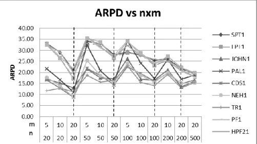
On the other hand, we can observe in Figures 12 and 13 the behavior of these procedures with the size of the instance (nxm). Figure 12 shows the performance of the heuristics with allocation method 1, and Figure 13 shows the group of heuristics using allocation method 2. Notice that the most influential factor in both groups is the number of machines per flow shop (m). When m
Figure 12. Behavior of heuristics with allocation method 1, with n x m
Figure 13. Behavior of heuristics with allocation method 2, with n x m
With respect to the heuristics using allocation method 3, Table 3 shows the ARPD for each heuristic and number of factories. Here, the best heuristic ranking has changed. Remember that, in this case, the sequence of jobs is divided into F parts, and each of these parts is assigned to one line. This situation is totally different from that which used the two allocation methods in the previous group. This explains the good performance of the three sequencing rules proposed for the blocking flow shop problem (PF, HPF2 and PW) as compared to the others proposed for the DPFSP. These methods sequence the jobs in order to minimize the idle time of machines, and
this order is maintained in the segment assigned to each line. From this group, we select PF3 and HPF23, which have similar performance. The overall ARPD is 10.50 and 10.55, respectively.
Heuristics Number of Flow shops
2 3 4 5 6 7 All SPT3 9.51 12.26 13.01 14.16 15.54 15.60 13.34 LPT3 9.84 11.86 13.21 13.92 15.11 14.88 13.14 JOHN3 11.16 14.22 16.39 17.22 17.85 18.75 15.93 PAL3 11.87 14.59 16.31 17.18 17.81 17.93 15.95 CDS3 11.49 14.36 16.20 17.15 17.88 17.82 15.82 NEH3 8.87 11.21 12.58 13.88 14.12 14.78 12.57 TR3 12.09 14.98 16.80 18.19 19.00 18.96 16.67 PF3 7.51 9.02 10.56 11.37 12.44 12.41 10.55 HPF23 7.16 8.92 10.26 11.39 12.51 12.75 10.50 PW3 8.61 10.46 11.82 13.30 13.81 14.15 12.03 Table 3. ARPD values by heuristic and number of factories in group 2
By analyzing the performance of this group of heuristics with respect to the size of the problem, we could see behavior that was similar to that in the heuristics with allocation methods 1 and 2. Their performance was mostly influenced by the size of m. They performed better for 20 machines than for 5, although we could also observe a slight effect of n, since their performance slightly improved when n increased.
Finally, the ARPD of the last group of heuristics is shown in Table 4. As can be seen, heuristics RC1_1 and RC1_m perform better than RC2. In particular, RC1_m is the one with a smaller ARPD. This means that, during the allocation process of jobs, it is better to select the flow shop which has the last machine available sooner.
Heuristics Number of Flow shops
2 3 4 5 6 7 All
RC1_1 7.71 10.63 12.14 13.58 14.27 15.13 12.24 RC1_m 7.74 9.74 11.29 12.80 14.30 14.55 11.74 RC2 9.72 11.76 13.06 13.73 15.77 16.21 13.38 Table 4. ARPD values by heuristic and number of factories in group 3
For this last group, in analyzing the performance of the heuristics with respect to the size of the problem, we saw behavior that was similar to that in the previous groups, except for the set of instance with n=100, where the performance is better for m=5 than for m=20. The improvement in this group when the number of jobs increases is more evident than in the other groups.
It is worth noting that the RPD values obtained in this test are very high, which indicates that the solutions obtained by these procedures are far from the best solutions used in this research. However, these best solutions were obtained by the ILS and IGA heuristics presented in this
Next, in order to compare the best two heuristics of each group, we carried out a multifactorial ANOVA on the results of these heuristics and all instances. The hypotheses of ANOVA were checked and satisfied. The response variable is the RPD, and the factors are the
Heuristics, n, m and F. This test shows us that all factors were significant (p-value=0.00).
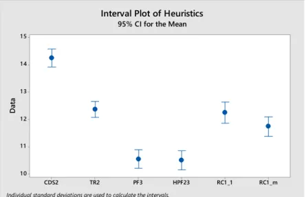
To analyze the differences between heuristics, we built the corresponding mean plot with the confidence interval at 95% for the heuristic factor (Figure 14), which is the most significant. As can be seen, the best heuristics are PF3 and HPF23. There are no statistically significant differences between them, because their confidence intervals overlap; nor are there significant differences between RC1_m, RC1_1 and TR2.
Figure 14.Interval Plot of compared heuristics at 95% confidence
A second analysis is necessary for evaluating heuristic efficiency, and that concerns the CPU time required for reaching the solution. Table 5 shows the average CPU time in milliseconds for each procedure and number of factories. The algorithms that consume the least time are those that use allocation methods 1 and 2. Next is the RC1 group. Finally, the algorithms that consume the most time are those that use allocation method 3. Remember that, in this method, the segment of the original sequence is first assigned to each plant, and then the insertion procedures are applied in order to improve the sequence. This helps in obtaining a high quality solution, but the required CPU time increases considerably.
RC1 _m RC1 _1 HPF23 PF3 TR2 CDS2 1 5 1 4 1 3 1 2 1 1 1 0 D at a
95% CI for the Mean
Individual standard deviations are used to calculate the intervals.
Heuristics Number of Factories 2 3 4 5 6 7 All TR1 2.6 2.6 2.5 3 3 3 2.7 CDS1 7.2 7.2 7.2 7.2 7.2 7.2 7.2 TR2 3 3 2.9 2.9 2.9 2.9 2.9 CDS2 7.2 7.2 7.2 7.2 7.2 7.2 7.2 PF3 226 103 59.6 39.3 28.3 22.4 79.6 HPF23 238 114 70.1 49.8 38.9 32.5 90.5 RC1_1 10.2 10.1 10.5 44.8 34.2 27.1 22.8 RC1_m 10.1 10.1 10.2 44.9 34.2 27.4 22.8
Table 5. Average CPU time in milliseconds, by heuristic and number of factories.
Hence, from the overall ARPD point of view, we could select HPF23 or PF3 as the best heuristics. However, RC1_m and TR2 cannot be discarded as initial heuristic solution procedures, because they obtain quite good solutions with less CPU time. Therefore, we implement three variants for each ILS and IG algorithm. Each variant uses HPF23, RC1_m and TR2, respectively. We denoted each variant with the name of the improvement heuristic plus the name of the constructive procedure used.
5.2
Experimental Parameter Adjustment of ILS and IG Algorithms
The proposed ILS and IGA have four parameters to be adjusted: the number of iterations in the
Reassignment and Permutation functions (nintlim), the number of jobs extracted from the current
solution in the Perturbation Mechanism (d), the Temperature in the Acceptance Function (Temp) and the initial solution procedure (solini).
The instances used in this experiment were a subset of the instances used in the calibration of the constructive heuristics. In this case, we used 100 instances grouped into 20 sets of size n x m, 5 instances per set, where n= {25, 50, 100, 200, 400} and m = {5, 10, 15, 20}. All these 100 instances were considered with a different number of parallel flow shops F={2, 4, 6}, which gave us 300 instances in total.
Both algorithms used the CPU time as the stopping criterion and limited it to 20•n2•m
milliseconds. The performance of the algorithms was measured with the RPD index calculated as (18). In this case, Cmaxh,k is the average makespan obtained by heuristic h, which is the heuristic that results from combining given values of parameters, in 5 runs in instance k, and Bestk is the minimum makespan obtained in this instance by any combination of parameters.
At this point, there are 60 combinations of n (5), m (4) and F (3) to be considered, as well as a number of parameters to adjust and a lack of any previous knowledge about their behavior; therefore, we decided to adjust the parameter values by employing a sequential experimentation
experiments based on the results of this first one will allow better adjustment than when running a single macro experiment.
Notice that –from the experiment’s point of view– n, m and F are basically blocking factors. We include them in the design because we want to get rid of the variability they introduce in the response when estimating the effect of the parameters.
For the initial experiment, we considered the following parameter levels for each algorithm (Table 6).
IGA ILS
Parameter Low level High level Low level High level
nintlim 50 75 50 75
d 5 6 6 7
Temp 0.4 0.6 0.4 0.6
Solini HPF23 RC1_m HPF23 RC1_m
Table 6. Parameter level for the first design
Given the 60 combinations of n, m and F, the 5 instances for each of combination and the 16 combinations of the parameters of interest (four parameters at two levels), a full factorial experiment implies 4800 runs.
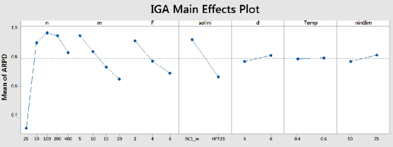
For the IGA algorithm, the results can be summarized in the main effects plot in Figure 15.
Figure 15. Main effects plot for IGA parameters
Aside from n, m and F being significant (as expected), the initial solution procedure (solini) is the only factor with a large effect, and it is clear that HPF23 is much better than RC1_m. The effects of d and nintlim are also significant, although small; and Temp appears to be inert. The only significant interactions, again as expected, are the ones involving n, m and F with some of the parameters. However, there are no significant interactions among the parameters. This is an important finding for setting up the second experiment.
Figure 16. Main effects plot for ILS parameters
A similar analysis for the ILS algorithm (Figure 16) provides the following conclusions: Again, aside from n, m and F, the initial solution (solini) is the only factor with a large effect and, again, it is clear that HPF23 is much better than RC1_m. This time, nintlim and Temp are inert, and d has a very small but significant effect. Again, there are no significant interactions among the parameters.
Given that the first experiment provided very similar results for both algorithms, we decided to use the same follow-up design in both cases. The idea was to use the findings from the first experiment to design a new set of trials that will help optimize the algorithms further. To do so, we took into consideration that solini does not interact with other parameters and fixed it at the best level while Temp, which is clearly inert, was also fixed. d and nintlim were the two parameters that deserved further attention, as they were significant but with a small effect. Then, the idea was to test more levels (3) that were also farther apart in order to see whether this would allow us to obtain larger effects that help optimize the algorithm further. The new levels are shown in Table 7.
Algorithm IGA ILS
Parameter Low Middle High Low Middle High
nintlim 30 40 50 30 40 50
d 3 4 5 4 5 6
Table 7. Parameter values for each algorithm
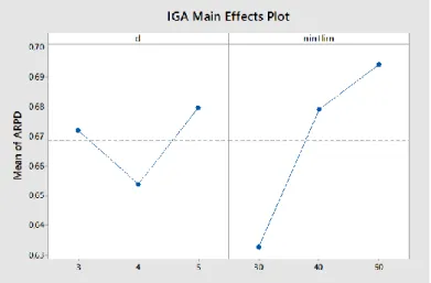
The results for the IGA algorithm, which is summarized in Figure 17, show that nintlim is very significant (p-value = 0.000) while significance is not so clear for d (p-value = 0.069). The two parameters do not interact, and thus their levels can be fixed at 4 for d and 30 for nintlim. The interaction between n, d and nintlim is significant, although with a very small effect that does not affect the conclusions.
Figure 17. Main effects of nintlim and d. Second experiment.
For the ILS algorithm, the results are simpler and contrariwise: d is highly significant (p-value
= 0.000) and nintlim is not significant (p-value = 0.229). There is a significant interaction between n and d, but it does not affect the conclusion that d=4 is the best one for all n. Figure 18 shows the results.
Figure 18. ILS effects plot
5.3
Computational Evaluation of the Heuristics
In this section we evaluate the general performance of the algorithms on two sets of instances. The first set includes small-sized instances that were also solved by the mathematical model proposed in this paper. The second set allows us to test the general performance against a larger benchmark; in this case, we once again used the well-known Taillard benchmark. We implemented the MILP model in CPLEX 11.1 commercial solver. All of the algorithms were encoded in the same language (QB64) and were tested on the same computer: an Intel Core 2 Duo E8400 CPU, with 2.5GHz and 2GB RAM memory.
5.3.1 Evaluation of the algorithms in small-sized instances
The general performance of the algorithms was evaluated with a set of small-sized instances that were generated ad-hoc. These instances were combinations of n={8,10,12, 14, 16}, m={2,
3, 4} and F={2, 3, 4}. There were 45 combinations of n, m, F. We generated 5 instances of each combination for a total of 225 instances. The processing time was uniformly distributed over [1, 99], as is normally done in the scheduling literature.
The model was run with a maximum CPU time of 5 hours, since our objective was to obtain the greatest number of optimal solutions in order to be able to compare the algorithms against them.
The heuristics were encoded in the same language (QB64) and were tested on the same computer: an Intel Core 2 Duo E8400 CPU, with 2.5GHz and 2GB RAM memory. To make a fair comparison, all heuristics adopted the CPU time limit as a stopping criterion, which was fixed at 30•n2•m•10-5 s. In each test, 30 runs were carried out for each algorithm on all 225 instances in order to see the differences between them. To analyze the experimental results obtained, we measured the RPD from the optimal solution if it was obtained by the model; otherwise, it was measured from the best known solution obtained by any of the algorithms in any run.
We found the optimal solution for all instances with 8, 10, 12 and 14 jobs and any combination of m and F. However, the instances with 16 jobs were the hardest; hence, we could solve only 60% of the instances within the maximum CPU time given. Therefore, from the 225 instances, we obtained 207 optimal solutions.
Table 8 shows the main results of this test. Notice that we have summarized the 1350 results for each set of n (45 instances per set x 30 runs each instance). The rows labelled “# of non-optimal” indicates the number of times the algorithm could not find the optimal solution. Those labelled “Mean RDP” are the average RPDs obtained in each set of 1350 results. Observe that, for the instances of 8, 10 and 12 jobs, almost all heuristics reach the optimal solution each time; and that it is for the instances with 14 and 16 jobs where we can see some differences between them. On top of the very high proportion of times in which the optimal solution was attained by all heuristics, it is worth noting the very low values of RPD obtained by those that did not reach the optimum.
Moreover, although the differences between heuristics are small and at this point non-significant, Table 8 also indicates that the IGA have a tendency to perform better than ILS.
n Legend IGA HPF23 IGA RC1_m IGA TR2 ILS HPF23 ILS RC1_m ILS TR2 8 # of non-optimal 0 0 0 0 0 0 Mean RPD 0 0 0 0 0 0 10 # of non-optimal 0 0 0 5 3 2 Mean RPD 0 0 0 0 0 0.0015 12 # of non-optimal 0 1 0 4 3 3 Mean RPD 0 0 0 0.0002 0.0005 0 14 # of non-optimal 18 11 9 34 26 40 Mean RPD 0.0036 0.0013 0.0008 0.0055 0.0068 0.0077 16 # of non-optimal 56 77 70 126 130 159 Mean RPD 0.0277 0.0234 0.0150 0.0400 0.0261 0.0417 All # of non-optimal 74 89 79 169 162 204 Mean RPD 0.0062 0.0049 0.0032 0.0092 0.0067 0.0102
Table 8. Summarized results of heuristics for
n
5.3.2 Evaluation of the algorithms in large-sized instances
Finally, we have analyzed the general performance of the heuristics with a set of large-sized instances. In this test, the heuristics were compared with two algorithms proposed for the DPFSP, which have been adapted to deal with the blocking constraint. They are the IGA proposed in Fernandez-Viagas and Framinan (2014) (named here IGA0) and the Scatter Search (SC) proposed in Naderi and Ruiz (2014). These algorithms were also coded in QB64 and were tested on the same computer. Once again, the comparison was made using the well-known Taillard’s benchmark. To make a fair comparison, all algorithms adopted the CPU time limit as a stopping criterion, which was fixed at k•n2•m•10-5 s, with k set to 15 and 30 in order to analyze the performance of these algorithms for two levels of CPU time. In each test, five runs were carried out for each algorithm on all instances. To analyze the experimental results obtained, we measured the RPD from the best known solution obtained during this research.
Table 10 shows the average RPD for each algorithm and number of parallel flow shops (F) when k=15. Notice that these results are considerably better than those obtained with the constructive procedures (Tables 4, 5 and 6), which indicate the good performance of the improvement phase that leads to better solutions. From these results, we can see that the three presented IGA perform better than the ILS. Moreover, one can observe that these three ILS perform similarly, with a slight advantage being had by the one that uses the RC1_m procedure to generate the initial solution. However, the differences between the presented IGA are greater, with an advantage being had by the one that uses the HPF23 to generate the initial solution. Notice that any variant of the presented ILS and IGA performs better than the algorithms IGA0 and SC that were proposed for the DPFSP, which we have further adapted in order to deal with the blocking constraint.
One of the main differences between the IGA0 and the IGA proposed here is the initial solution procedure. IGA0 uses NEH2, which did not show good performance for the blocking case when compared with the procedures that are presented here and which, in addition, take into account the characteristics of the problem. Another difference is that our IGAs use a variable neighborhood search to improve the sequence of jobs assigned to each line, not only when the initial solution is created but also after the perturbation mechanism is implemented, which helps to obtain a better solution. Finally, the type of search in the reassignment is also different. In IGA0, the local search is exhaustive, i.e., when it tries to insert a job into another factory, all positions are tested and the best is kept; whereas, with our method, the first position that leads to a better makespan is kept and the search begins again. The non-exhaustive search is more efficient when the time is limited, because it allows conducting more trials, which allows exploring a larger neighborhood area.
F IGA0 IGA HPF23 IGA RC1_m IGA TR2 ILS HPF23 ILS RC1_m ILS TR2 SC 2 1.811 0.934 1.392 1.277 1.413 1.295 1.711 2.424 3 1.798 0.861 1.203 1.118 1.313 1.167 1.383 2.677 4 1.778 0.813 1.083 0.994 1.269 1.168 1.263 2.999 5 1.404 0.765 0.932 0.845 1.214 1.122 1.135 3.063 6 1.355 0.873 0.854 0.773 1.173 1.121 1.095 3.144 7 1.326 0.818 0.809 0.691 1.143 1.105 1.047 3.160 Average 1.579 0.844 1.046 0.949 1.254 1.163 1.272 2.911
Table 9. Average RPD by algorithm and number of factories with k=15
To confirm the results of Table 9 and to study the convergence of algorithms, we ran all the algorithms again while allowing more CPU time. In this case, we set it at k=30. Table 10 shows the obtained average RPD by number of factories. As can be observed, all of them improved their performance considerably, especially the presented IGAs. Notice that IGA_HPF23 has better performance with a lower ARPD; but when the number of lines to consider increases, its efficiency decreases slightly. This is the opposite of IG_TR2, which performs better with a larger number of parallel flow shops.
F IGA0 IGA HPF23 IGA RC1_m IGA TR2 ILS HPF23 ILS RC1_m ILS TR2 SC 2 1.528 0.659 0.977 0.899 1.141 1.050 1.327 2.005 3 1.502 0.596 0.815 0.779 1.053 0.942 1.095 2.279 4 1.526 0.552 0.741 0.685 1.010 0.952 1.022 2.547 5 1.128 0.517 0.616 0.588 0.986 0.926 0.912 2.644 6 1.132 0.622 0.589 0.525 0.965 0.935 0.902 2.716 7 1.160 0.572 0.536 0.484 0.949 0.928 0.865 2.805
To perform a deeper analysis, the results were analyzed by means of a multiway analysis of variance (ANOVA), where n, m and F were non-controllable factors. To check the ANOVA model hypothesis (normality, homoscedasticity and independence), the standardized residuals were analyzed and no major departure from the assumption was found. The test showed us that
n, m, F, Heuristics and their interactions were significant (p-value=0), which means that the heuristics do not have the same behavior for each group of n, m and F values, as we already saw in Tables 9 and 10.
Figure 19 shows the main effects plot for ARPD. In this figure, we can see that the heuristics obtain better results on average. These results are close to the best known makespan for lower values of n and for larger values of m, which is a result already found in the permutation flow shop problem, i.e., where F=1. Moreover, as we see in Table 9 and 10, the heuristics perform better on average when F increases. This is probably due to each line having a lower number of jobs to schedule, which leads to a better solution even though the complexity increases during the search as a result of there being more lines to reassign the jobs during the improvement phase.
Figure 19. Main effects plot for ARPD
Finally, Figure 20 shows the confidence interval plot of RPD for the three IGAs presented in this paper. Remember that the only difference between them is the implemented initial solution procedure. Notice that the differences between the algorithms are significant. From these results, we can confirm that IGA_HPF23, whose initial solution was specifically designed for the problem on hand, is the best performing algorithm for this problem. This indicates that the
blocking constraint makes quite an important difference with respect to the permutation problem, which implies that the algorithms need to be designed especially for dealing with it.
Figure 20. Interval plot for RPD by each IG variant.
6
Conclusions
This paper presents and compares some constructive procedures and heuristic algorithms for dealing with both the parallel blocking flow shop problem (PBFSP) and the distributed blocking flow shop problem (DBFSP). The procedures for solving these problems have to not only consider rules for sequencing the jobs, but also assign them to the parallel flow shops (factories). The implemented constructive procedures have allowed us to test three different strategies, two of them designed especially for dealing with the blocking. From the analysis of results, we have concluded that one good strategy is to generate a sequence of jobs by trying to minimize the front delay and the timeout of machines, and to then divide the sequence with segments that have a similar workload in order to assign each job to one of the factories (HPF23). Another strategy is to consider the job and the line at the same time in order to assign the job to the line with the last machine available before all the others (RC1_m).
The heuristic procedures presented here are variants of an iterated greedy algorithm (IGA) and an iterated local search (ILS) algorithm, both of which are combined with a variable neighborhood search (VNS). The variants consist of different constructive procedures for generating the initial solution. In particular, we have selected three constructive procedures from among the ones that have been implemented, i.e., the best one from each strategy tested. As, to the best of our knowledge, this is the first attempt to propose heuristics for the PBFSP (DBFSP), we adapted two algorithms proposed for the DPFSP in order to compare our algorithms against
IGA_TR2 IGA_RC1 _m IGA_HPF23 0.75 0.70 0.65 0.60 0.55 D at a
95% CI for the Mean
Individual standard deviations are used to calculate the intervals.