Bioinformatics analyses of alternative splicing, est-based and machine learning-based prediction

(1)

BIOINFORMATICS ANALYSES OF ALTERNATIVE

SPLICING, EST-BASED AND MACHINE LEARNING-BASED

PREDICTION

by

JING XIA

B.E., Shanghai Jiaotong Univeristy, China, 2006

A THESIS

submitted in partial fulfillment of the

requirements for the degree

MASTER OF SCIENCE

Department of Computing and Information Sciences

College of Arts and Sciences

KANSAS STATE UNIVERSITY

Manhattan, Kansas

2008

Approved by:

Major Professor William Hsu

(2)

Copyright

Jing Xia

(3)

Abstract

Alternative splicing is a mechanism for generating different gene transcripts (called iso-forms) from the same genomic sequence. Finding alternative splicing events experimentally is both expensive and time consuming. Computational methods in general, and EST analy-sis and machine learning algorithms in particular, can be used to complement experimental methods in the process of identifying alternative splicing events. In this thesis, I first iden-tify alternative splicing exons by analyzing EST-genome alignment. Next, I explore the predictive power of a rich set of features that have been experimentally shown to affect al-ternative splicing. I use these features to build support vector machine (SVM) classifiers for distinguishing between alternatively spliced exons and constitutive exons. My results show that simple, linear SVM classifiers built from a rich set of features give results comparable to those of more sophisticated SVM classifiers that use more basic sequence features. Finally, I use feature selection methods to identify computationally the most informative features for the prediction problem considered.

(4)

List of Figures

1.1 Chemical structure of DNA helix . . . 5

1.2 Illustration of main stages of gene expressions . . . 6

1.3 Illustration of the splicing process . . . 7

1.4 Example of alternatively spliced genes in C. elegans . . . 9

1.5 Illustration of five kinds of alternative splicing patterns . . . 10

2.1 Illustration of support vectors and marginBur98 _{. . . .} ₁₇

2.2 Linear hyperplane for non-linear separable case . . . 21

2.3 Example of mapping input spaces to feature spaces . . . 22

2.4 Example of weighted degreeed kernel . . . 24

2.5 Example of weighted degree kernel with shifts . . . 25

4.1 Comparison of ROC curves with different combination of features . . . 39

4.2 AUC score comparison between data set with different features . . . 40

4.3 AUC scores comparison between data sets with features of secondary struc-ture and data sets without feastruc-tures of secondary strucstruc-ture . . . 41

(7)

List of Tables

1.1 A brief history of genetics . . . 3

1.2 Basic steps of gene expression . . . 6

2.1 Programs for spliced-sequence to genome DNA alignment . . . 14

4.1 Number of occurrences and percentage for each alternative splicing event. . . 34

4.2 Intersection between MAST motifs and ISR motifs . . . 35

4.3 Results of alternatively spliced exons classification. All features, but ISR motifs, are included. . . 37

4.4 Results of alternatively spliced exons classification. All features, including ISR motifs are used. . . 38

4.5 Weight importance of the following features . . . 40

4.6 List of mastk, esek and irsk motifs found by choosing nodes which occur in all decision tree classifiers . . . 42

(8)

Acknowledgments

I would like to thank Dr. Doina Caragea as my committee member for continuous support. Also, I would like to thank Dr. William H. Hsu as my major professor for guiding my thesis workwith his helpful advice. I also want to be grateful to Dr. Susan Brown at KSU for her guide in my thesis work. This work will not be done without their support. Furthermore, I want to thank Hee Shin Kim at the Bioinformatics Center at Kansas State University, Dr. Caragea and Wesam Elshamy for proof reading the draft and for helpful discussions. I acknowledge the support from the KDD group at Kansas State University. Part of this work was supported by the National Science Foundation under Grant No. 0711396. Last, but not least, I want to thank my little girlfriend Wen for being the greatest.

(9)

Dedication

(10)

Preface

Hereby, I would like to record my research experience during my master graduate study. The work described in this thesis started as a class project forthe Introduction to Bioinfor-matics course that I took at Kansas State University in Spring, 2007. I clearly remember Dr. Caragea (at KSU) mentioning in her class that there are still many open problems in current bioinformatics research and therefore great need for dedicated researchers. Being fascinated by biological pheonomena, I chose one of these topics, pre-mRNA Alternative Splicing, as my class project and continued to work on same problem during my master studies.

Pre-mRNA splicing is a complicated process through which genes remove specific pieces from their sequence, so-called ”non-use” RNA, in order to form the final coding messenger RNA. Then, the mRNA is transported to cytoplasm for protein formation. The whole procedure is highly regulated by signals and regulators, known or unknown to scientists, in a single cell. The splicing process can vary a lot under different conditions, resulting in different final products (i.e. which pieces of RNA will be removed can be dependant on different environments).

It is fundamental because around 50% genes of human beings undergo alternative splic-ing, but there is still no theory for predicting and interpreting the process. What is known is that a number of aspects of the sequence are correlated to AS. For an example, features such as exon and flanking intron size, splice site strength, mRNA secondary structure, or RNA editing, etc, can affect the AS products. With respect to computational approaches, there are exisitng algorithms in machine learning used to guide the computers to learn to predict alternative splicing events. Getting inspiration from two aspects, we tried to incorporate these biological background knowledge into computational approaches, in hope of getting a better classifier. And the results are published as a regular paper in the proceedings of BIBM 2008XCB08_.

(11)

Chapter 1

Introduction

In this chapter, we will provide the biological background underlying the process of alter-native splicing and then we will present the problems addressed in this work.

1.1

Overview

As well-known, DNA is the genetic code for human heritage. As many species’ genomes have been sequenced, the next question is how to find useful knowledge which explains biological phenomenon from these treasure. Central dogma of molecular biology is a process in which gene are transformed from DNA sequence to functional protein products with regulation rules and mechanism involved. One of the steps in the gene expression process is pre-mRNA splicing which refers to the process through which ”pieces” of the DNA sequence are removed or retained However, the splicing process is variable, depending on the type of tissue, where it takes place, conditions and so on. Under certain situations, pre-mRNa will remove different pieces from its sequence and splicing together alternatively. Thus, the same gene can result in several different mRNA isoforms products, which are translated into different gene products. Such biological phenomenon is defined as,Alternative Splicing (AS). Furthermore, some genes undergo AS events, while others do not. Understanding how to distinguish constitutively spliced genes1_{; from alternatively spliced genes is an important}

open research topic that scientists are interested in. This involves understanding the effect

(12)

of the environment in addition to understanding the internal mechanism of AS. The process of AS is one of significant problems which have not been fully understood. Here come the questions: how can we distinguish a AS gene from a constitutively spliced gene how to formalize external environment and internal mechanism in gene splicing and so on.

Thus, identifying AS events using wet lab experiments is both time consuming and ex-pensive, computational approaches have been often used to facilitate the research of AS problems in a different aspect. Here, we apply computational methods, in particular, Sup-port Vector Machines (SVM), to address an imSup-portant AS problem, specifically, the problem of distinguishing AS genes from constitutively spliced genes. The main idea in this work is to incorporate biological background knowledge of alternative splicing into computational approaches by using an appropriate biological feature representation. Further, we train an inducer to learn to classify genes into two classes, i.e. constitutively and non-constitutively spliced exons. More specifically, here we only consider constitutively and non-constitutively spliced genes in terms of skipped exons, one of AS patterns, i.e. we only consider whether genes contain exons can be skipped during splicing process.

1.2

Biological Background

The modern science of genetics traces its roots to Mendel, who started a new branch in biology,Genetics. In 1944, Oswald Theodore Avery, etc. identified the molecule responsible for the transformation of genetics bydeoxyribonucleic acid (DNA)AMM44_{. James D. Watson}

and Francis Crick determined the structure of DNA in 1953. One important development was chain-termination DNA sequencing in 1977 by Frederick Sanger: this technology allows scientists to read the nucleotide sequence of a DNA molecule. Recently, the completion of sequencing the genome of the nematode Caenorhabditis elegans at the end of 1998 and the first draft sequence of the human genome in June 2000 are significant milestone in history. Table 1.1 is a list of important events in history of genetics.

(13)

ex-1865 Genes are particulate factors 1903 Chromosomes are hereditary units 1910 Genes lie on chromosomes

1913 Chromosomes contain linear arrays of genes 1927 Mutations are physical changes in genes 1931 Recombination is caused by crossing over 1944 DNA is genetic material

1945 A gene codes for a protein 1953 DNA is double helix

1958 DNA replicates semiconservatively 1961 Genetic code is triplet

1977 DNA can be sequenced 1997 Genomes can be sequenced

1998 Completion of the genome of the Caenorhabditis Elegans 2000 ’Working Draft’ of the human genome announced

Table 1.1: A brief history of geneticsSRJM02

ist two kind of organisms in nature, eukaryotes and prokaryotes. The difference between eukaryotic and prokaryotic organisms is that the cells of eukaryotes contain nuclei and a cytoskeleton, while these are not present in prokaryotes. Eukaryotes are considered to be higher organisms since their biological mechanism is much more complicated than those of prokayotes. Human as well as C. elegans belong to the class of eukaryotes. Further, in nuclei, genetic information is conserved in form of chromosomes. The whole set of chro-mosomes, referred as genome, is organized as a collection of discrete, separable information packets, called genes. That means some pieces of chromosomes are non-informative or have unknown functionPea06. For instance, C. elegans has six pairs of chromosomes, one pair of which determines the sex. Hermaphrodite C. elegans, i.e. which has both male and female reproductive organs, has a matched pair of sex chromosomes (XX); the rare males have only one sex chromosome (X0). More detailed, a series of genes on chromosome X, not the whole chromosome, is correlated to sex determinationBre74.

Each chromosome is made of a long deoxyribonucleic acids (DNA) chain, which is the carrier of genes and regulatory elements. The DNA chain is constructed by millions of

(14)

pair-wise DNA bases, connecting together pair by pair to form a long double-stranded sequence. The backbone structure of connecting DNAs is made of phosphate and sugar residues. The sugar in DNA is a 2-deoxyribose and pentose (five-carbon) sugar. The sugars are joined together by phosphate groups that form phosphodiester bonds between the third and fifth carbon atoms of adjacent sugar rings. These asymmetric bonds give direction to a strand of DNAs has a direction. In addition to sugar and phosphate, there exist four kinds of nucleotide bases Adenine, Thymine, Guanine and Cytosine in DNA. In Fig. 1.1, there shows a chemical structure of DNA helix. As can be seen in the Figure, only the base pair Adenine-Thymine and Guanine-Cytosine may form by hydrogen bonds. And these pairs, connecting by phosphodiester bonds, form a double helix in 3D structure. The 5’ position of one pentose ring to the 3’ position of the next 3’ pentose ring gives a direction, which is written in 5’ to 3’ direction. And the two ends of the strand refers to 5’ ends and 3’ ends with respect to the direction of the strand. Due to the complementary base pairing, the two strands are anti-parallel, cf. Fig. 1.1.

A DNA sequence is a long chain of base pairs (i.e. A-T, C-G) which wrap up and compress, and eventually form a chromosome. A gene can be defined as a piece of region DNA sequence which controls a certain hereditary characteristic. However, most regions on the DNA sequence are non-genetic regions while the current estimated that genes in the human genome is just under 3 billion base pairs and about 20,000 ∼ 25,000 protein-coding genes. However, the gene density on the human genome is roughly 12∼15 genes per one megabase pairs. Having explained the DNA structure, next we will briefly introduce the following concepts:

1. the main steps of the gene expression process in eukaryotes

2. biological phenomena of alternative splicing which can be seen as the exception to the standard splicing steps in genes expression process.

At high-level, the process of gene expression in eukaryotes consists the following main steps, Activation of proximal promoters, initiation of transcription, transcription and

(15)

ter-Figure 1.1: The chemical structure of DNA helix. Four basic DNA molecules, Adenine, Thymine, Guanine, Cytosine, form two pairs (A-T, C-G) which connect through hydrogen bonds,. The two sugar rings on one-stranded side form the backbone which is held together through phosphate bonds. Each strand has a direction. The left-sided strand is from 5’ to 3’ while the right strand is from 3’ to 5’ and they are anti-parallel.

mination, splicing, translocation, and translation. Table 1.2 comments the steps of the gene expression process and the products in their corresponding phase. These steps will be described into more details in what follows.

Unlike DNA replication, transcription does not need a primer to start. RNA polymerase binds to the DNA with other cofactors, and unwinds the DNA to create a bubble that makes it possible for RNA polymerase to read one of the double-stranded DNA template. In eukaryotes, a collection of proteins called transcription factors mediate the binding of RNA polymerase and the initiation of transcription. Only after certain transcription fac-tors are attached to the promoter, RNA polymerase can also bind. With the proceeding of the RNA polymerase bubble, staring from the Transcriptional Starting Site (TSS) to termination point, a copy of DNA, called precursor messenger ribonucleic acid (pre-mRNA)

(16)

Stages Products 1. Activation of proximal (core) promoters Initialized DNA

and initiation of transcription

2. Processing of transcription and termination pre-mRNA

3. Post-transcriptional modification mRNA in nucleus 4. Translocation of mRNA to cytoplasm mRNA in cytoplasm 5. Translation of mRNA into proteins protein

Table 1.2: Basic steps of gene expression

is synthesized; However, the base Thymine in the DNA template is replaced by the base Uracil (U) in the pre-mRNA synthesis.

exon intron exon intron exon

5’UTR GT AG GT AG 3’UTR

exon intron exon

5’UTR TSS ATG cap GU intron exon AG ATG GT AG _3’UTR DNA Trasncription pre−mNRA mRNA protein Splicing Translation

Figure 1.2: Illustration of main stages of gene expressions

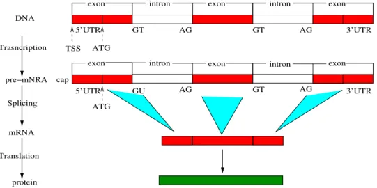
The next step in the process is the post-transcriptional stage in which the pre-mRNA is transformed into mature mRNA through theSplicing mechanism. The pre-mRNA contains non-coding regions calledintrons which are interspersed among coding regions called exons. The pre-mRNA sequence starts with an exon and followed by an intron, and then another exon, etc. and it ends with the last exon. Fig. 1.2 shows the main stages of the gene expression process. As we can see, the boundaries between exons and introns, called splice sites, have strong consensus sequences. The exon-intron splice sites (i.e., 5’ splice sites of introns), called donor sites, show a consensus sequence, GU, while the other end of

(17)

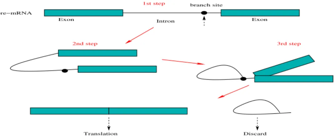
introns (i.e., 5’ splice sites of introns), called acceptor sites, have the sequence of consensus of AG. The major process of splicing is a series of protein complexes, called spliceosomes as catalysts. With the help of spliceosomes, an intron is bent and move to 3’ splice site, forming a loop structure. Next, the 5’ splice site is cleaved and bound to one specific site in the intron, called branch site, resulting in the formation of an intron lariat structure. The branch site shows a consensus base,Aand is nearly upstream the 3’ splice site. Further, the 3’ splice site is further cleaved and the two exons are ligated with the help of spliceosomes. At last, the spliced intron is released and the mRNA is synthesized. Fig. 1.3 illustrates briefly how an intron is spliced out from the sequence.

Exon Intron Exon

1st step

pre−mRNA

branch site

2nd step 3rd step

Translation Discard

Figure 1.3: Illustration of the splicing process

After the pre-mRNA is transformed into mRNA, it will be transported from nucleus to cytoplasm where ribosomes are located. Ribosomes are chemical complexes which surround the mRNAs and function as catalysts in the process of translating the mRNA template into the final products,proteins. The mRNA is read in a sequence of triplets, calledcodons. While reading the codon codes, the ribosome and transfer RNA (tRNA) translate the codons into a chain of amino acids until the termination codon is reached. The amino acids join together to form protein, which is a long polypeptide, held together by peptide bonds. Sixty one out of a total sixty four (43 _{= 64) possible codon code for twenty amino acids, while the}

(18)

the process of DNA transcription, translation also starts at the start codon AUG, called translation initiation site (TIS). We end here our brief description of the gene expression process and will focus an exception to this process next.

As many precesses, the process of gene expression has a lot of exceptions in nature, and pre-mRNA alternative splicing is among one of these well-known exceptions. For years, it was believed that one gene corresponds to one protein, but the discovery of alternative splicingGil78 _{provided a mechanism for generating different gene transcripts (isoforms) from}

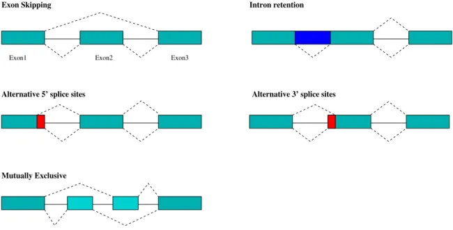
the same genomic sequence. Fig.1.5illustrates five main kinds of AS patterns and shows how isoforms differentiate from each other. Years after its discovery, alternative splicing was still seen more as the exception than the ruleAst04_{. Recently, however, it has become obvious that}

a large fraction of genes undergoes alternative splicingGra01_{. Early analyses suggested that at}

least 50% of human genes undergo alternative splicingint,ven_{. More recently, approximately}

75% of human genes appear to be alternatively splicedJCGE+₀₃

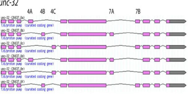
. Alternate splicing occurs in many other organisms. Approximately 20% of the predicted genes in Drosophila species have been shown to undergo alternative splicingLTR04, some of which can produce a very large number of isoforms. For example, Drosophila’s Dscam gene could in principle produce up to 38,016 isoformsSCS+00 and this diversity is essential for neuronal wiring and self-recognitionDEH+07. Another example is the unc-32O gene in model organism, C. elegans that can be alternatively spliced to six different transcripts isoforms (1.4). As shown in the figure, exon 4 can undergo three different mutually exclusive AS, while two for exon 7 leading to six possible transcriptsZah05. On the other hand, aberrant splicing has been linked to pathological states such as cancerKTB+02. These results underscore the importance of alternative splicing, both in normal and aberrant conditions. However, the task of accurately identifying alternative splicing isoforms is particularly intricate, as different transcriptional isoforms can be found in different tissues or cell types, at different development stages or induced by external stimuli.

(19)

Figure 1.4: Example of alternatively spliced genes in C. elegans. Illustration of unc-32 in C. elegans undergo six alternative splicing. Images are taken from Wormbase genome browser

1.3

Problem specification

The task of accurately identifying alternative splicing isoforms is particularly intricate, as different transcriptional isoforms can be found in different tissues or cell types, at different development stages, or can be induced by external stimuli. Experimental methods for find-ing alternative splicfind-ing events are expensive and time consumfind-ing. Therefore, computational methods that can complement experimental methods are needed. Traditional computational methods rely on aligning expressed sequence tags (ESTs) and complementary DNA (cDNA) to genomic DNA to identify alternative splicing eventsNGR06,KRGS01_. _{The basic idea of the}

approach is based on the alignment transcripts to genome sequences, which identifies the gene loci and structures. AS events can be identified through further scanning the bound-aries of the genes. However, this approach is limited to both the quality and the coverage of the transcripts. More recently, machine learning approaches is used to predict alternative splicing events through ”learning” various sequence featuresRSS05a,WM06,SSC+04.

(20)

Exon1 Exon2 Exon3

Exon Skipping

Mutually Exclusive

Intron retention

Alternative 5’ splice sites Alternative 3’ splice sites

Figure 1.5: Illustration of five kinds of alternative splicing patterns. Lower-level dash lines connect exons, forming constitutively spliced isoforms, while upper-level dash lines connect exons alternatively, making an alternative spliced isoforms. According to its different spliced structure, five AS patterns are Exon Skipping, Intron Retention, Alternative 3’ Splice Sites, Alternative 5’ Splice Sites and Exon Mutually Exclusive

Although several types of alternative splicing events exist (e.g., alternative acceptor, alternative donor, intron retention), in this thesis we focus on the prediction of cassette ex-ons, one particular type of splicing event, where an exon is a cassette exon (or alternatively spliced) if it appears in some mRNA transcripts, but does not appear in all isoforms. If an exon appears in all isoforms, then it is called a constitutive exon. Several basic sequence fea-tures have been used to predict if an exon is alternatively spliced or constitutive, including: exon and flanking introns lengths and the frame of the stop codon. In particular, G. R¨atsch et al.RSS05a _{have proposed a kernel method, which takes as input a set of local sequences}

represented using such basic features and builds a classifier that can differentiate between alternatively spliced and constitutive exons. In the process of building the classifier, this method identifies and outputs predictive splicing motifs, which are used to interpret the results. In this context, a motif is a sequence pattern that occurs repeatedly in a group of related sequences. The method in the workRSS05a is essentially searching for motifs within a

(21)

certain range around each base. This range needs to be carefully chosen in order to obtain good prediction resultsHO08_.

Finding motifs that explain alternative splicing of pre-mRNA is not surprising as it has been experimentally shown that alternative splicing is highly regulated by the interaction of intronic or exonic RNA sequences (more precisely, motifs that work as signals) with a series of splicing regulatory proteinsHO08_{. Such splicing motifs can provide useful}

informa-tion for predicting alternative splicing events, in general, and cassette exons, in particular. Generally, computational identification of splicing motifs can be derived from patterns that are conserved in another organismKBSM+_{06,SA03,DSS05b}

. However, since some exons and most introns are not conserved, it is desirable to identify such motifs directly from local sequences in the organism of interest.

In addition to motifs, several other sequence features have been shown to be informative for alternative splicing predictionHO08_{. Among these, pre-mRNA secondary structure has}

been investigated to identify patterns that can affect splicingHZBS07,PYR02. It has been found that the pre-mRNA exhibits local structures that enhance or inhibit the hybridization of spliceosomal snRNAs to the pre-mRNA. In other words, the structure can affect the selec-tion of the splice sites. As another feature, the strength of the general splice sites is very important with respect to the splicing process, as strong splice sites allow the spliceosomes to recognize pairs of splice sites between long intronsWM06,FH07. When the splice sites degen-erate and weaken, other splicing regulatory elements (exon/intron splicing enhancers and silencers)PMS07 are needed. At last, one other feature that has been shown to be correlated with the spicing process is given by the base content in the vicinity of splice sitesHO08.

Although the method in the workRSS05a can output motifs that explain the classifier results, to the best of our knowledge there is no study that explores motifs (derived ei-ther using comparative genomics or local sequences) and oei-ther alternative splicing features (pre-mRNA secondary structure, splice site strength, splicing enhancers/silencers and base content) together as inputs to machine learning classifiers for predicting cassette exons.

(22)

In this thesis, we use the above mentioned features with state-of-the-art machine learning methods, specifically the SVM algorithm, to generate classifiers that can distinguish alterna-tively spliced exons from constitutive exons. We show that the classification results obtained using all these features with simple linear SVMs are comparable and sometimes better than those obtained using only basic features with more complex non-linear SVMs. To identify the most discriminative features among all features in our study, we use machine learning methods (SVM feature importance and information gain) to perform feature selection.

1.4

Organization

The rest of the thesis is organized as follows: We have introduced biological background relevant to our issue in Chapter 1.2, we will introduce computational methods to identify alternative splicing events, the machine learning algorithms used to predict alternatively spliced exons and to perform feature selection. In Chapter 3, we describe the data set used in our experiments and explain how we construct the features considered in our study. We present experimental results in Chapter 4 and conclude with a summary and ideas for future work in Chapter 5.

(23)

Chapter 2

Methods

2.1

Identifying AS events by analyzing EST data

Expressed sequence tags (EST) are short, around 200 ∼ 800 nucleotide bases in length, unedited, randomly selected single-pass sequence reads derived from cDNA libraryNGR06_.

Due to both the cost-effectiveness of generating ESTs and the value of the biological infor-mation, high-throughout of ESTs are used in a wide area of biology (gene discovery, gene structure identification, alternative transcripts detection, complement of genome annota-tion, single nucleotide polymorphism characterization and facilitation of proteome analy-sis)NGR06_{. On the other hand, the error-prone property of ESTs (caused by single pass and}

errors toward the ends of the reads) might cause false prediction of knowledge.

When ESTs are used to investigate alternative splicing, EST-mRNA comparisons, EST-genome alignment comparisons, andEST-genome multiple alignment comparisons are three computational methods and the latter two being more robust with respect to prediction accuracyBRP06_{. Overall, the main idea underlying all three kinds of methods is 1) to identify}

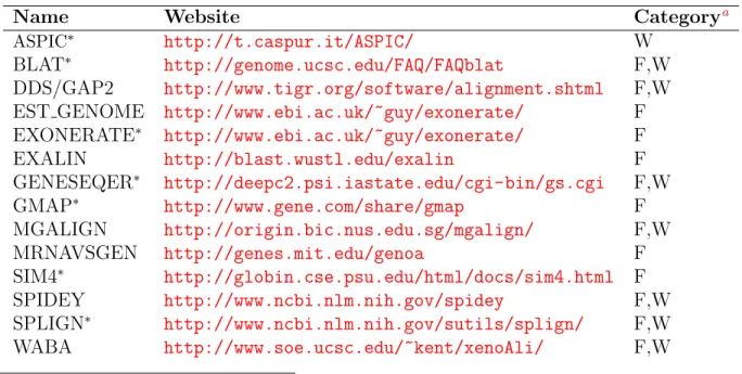
the gene structure by alignments of ESTs with genomic or transcript sequences, and then 2) to predict alternative splicing by looking for different transcript isoforms (i.e. patterns of alternative splicing) of one gene structure. A number of tools are available for automating the procedure of alignment of ESTs to genomic DNA (listed in Tabel2.1). The key algorithm underlying the sequence alignment is dynamic programming, DP, which can compute the

(24)

Name Website Categorya

ASPIC∗ http://t.caspur.it/ASPIC/ W

BLAT∗ http://genome.ucsc.edu/FAQ/FAQblat F,W

DDS/GAP2 http://www.tigr.org/software/alignment.shtml F,W EST GENOME http://www.ebi.ac.uk/~guy/exonerate/ F EXONERATE∗ http://www.ebi.ac.uk/~guy/exonerate/ F EXALIN http://blast.wustl.edu/exalin F GENESEQER∗ http://deepc2.psi.iastate.edu/cgi-bin/gs.cgi F,W GMAP∗ http://www.gene.com/share/gmap F MGALIGN http://origin.bic.nus.edu.sg/mgalign/ F,W MRNAVSGEN http://genes.mit.edu/genoa F SIM4∗ http://globin.cse.psu.edu/html/docs/sim4.html F SPIDEY http://www.ncbi.nlm.nih.gov/spidey F,W SPLIGN∗ http://www.ncbi.nlm.nih.gov/sutils/splign/ F,W WABA http://www.soe.ucsc.edu/~kent/xenoAli/ F,W

a_{F, free for academic users; W, web server avaiable; *, investigated in the research}

Table 2.1: Programs for spliced-sequence to genome DNA alignment

optimal sequence alignment in quadratic runtime and memory complexity. For an example, given an mRNA sequence and a genomic sequence, DP finds an alignment of the mRNA to the genomic sequence, which allows long gaps insertion into the mRNA sequence. Thus, gap penalties should be based on intron length distribution, and gaps following the rules of splice sites should be more preferredHO08_.

After genome-wide alignments are performed, the next step is the identification of consti-tutive and alternative exons as one type of alternative splicing patterns. Consticonsti-tutive exons are in default splicing isoforms, while exons that are as annotated alternatively spliced, should meet specific conditions. After identifying the splicing junctions (i.e. putative splic-ing sites), one can order them with respect to gene loci to construct a matrix of splicsplic-ing junctions, in which exons are considered as nodes and splicing junctions as edges connecting nodes. Traversing through this adjacent-matrix graph will capture the alternative splicing eventsKSG02_.

(25)

This approach based on ESTs analysis is widely used for identifying AS events. However, there are some limitations to the approach, which are mainly from both the error-prone property of ESTs and the limited coverage of ESTs for newly sequenced genome. These limitations will result in making false positive identification of AS events and missing AS events. And this approach can not be used to predict AS events for genes. Thus, ,ore recently, machine learning based approaches are used to do the task of predicting AS events. Next, we will introduce one of the machine learning algorithms, Support Vector Machines (SVM) and how to adapt this advanced algorithm to the problem of predicting AS events.

2.2

Support Vector Machine Classifiers

The support vector machine (SVM) algorithmVap99 _{is one of the most effective machine}

learning algorithms for many complex binary classification problems, including a wide range of bioinformatics problemsGWBV02,LEC+_{03,BHB03,PMS07}

, and has been recently used to detect splice sitesRS04,RSS05a,SSP+₀₇

. The SVM algorithm takes as input labeled data from two classes and outputs a model (a.k.a., classifier) for classifying new unlabeled data into one of those two classes. SVM can generate linear and non-linear models.

Let E = {(x1, y1),(x2, y2),· · · ,(xl, yl)}, where xi ∈ Rp and yi ∈ {−1,1}, be a set of training examples. Suppose the training data is linearly separable. Then it is possible to find a hyperplane that partitions the pattern space into two half-spaces. Suppose there is one for the linearly-separable data set. The classifier is defined as a function f :x→ {−1,+1} that predicts the labelyi of anyxi ∈Rp . SVM algorithm learns to construct above defined decision function from the set of training examples, E in the form of a linear separating hyperplane. We have

f(x,w, b) = sign(w·x+b) (2.1)

The set of such hyperplanes is given by {x|x·w+b= 0}, wherexis thep-dimensional data vector and w is the normal to the separating hyperplane. The learning task is to find the normal weights w and the biasb.

(26)

2.2.1

The Separable Case

Firstly, we assume that the training examples can be separated by a linear hyperplane as defined in Eq. (2.1). SVM selects among the hyperplanes that correctly classify the training set, the one that maximizes the margin between positive and negative examples, subject to certain constraints such that:

w·x+b≥+1 f or yi = +1 (2.2)

w·x+b ≤ −1f or yi =−1 (2.3)

⇒yi(xi·w+b)≥ ±1f or yi =±1 (2.4)

We denote the plus hyperplane as H1 and minus hyperplane as H2, both of which are

parallel to the decicsion boundary H=x·w+b = 0.

H1 : w·x+b = +1

H2 : w·x+b=−1

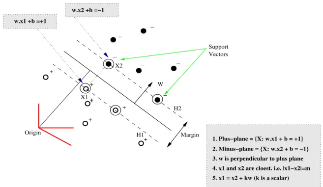
The perpendicular distance between these hyperplanes is given by _||w||2 , which is called margin. SVM chooses one minimal normal ||w|| which maximizes the margin and also satisfies the constraint Eq. 2.4. For an example of support vector machines, Fig 2.1 shows maximal margin between the hyperplanes of two classes. We derive formula _||w||2 , the distance

What we know: Induction: Induction Cont. : (1) w·x1+b = +1 Based on (1) & (3) Based on (4) & (5) (2) w·x2+b =−1 ⇒w·(x2+λw) +b= 1 M =|x1−x2|=|λw| (3) x1 =x2+λw ⇒w·x2+b+λw·w= 1 =λ|w|=λ√w·w (4) |x1−x2|=M ⇒ −1 +λw·w= 1 = 2 √ w·w w·w = 2 √ w·w ⇒λ= _w·w2 (5) = _|w|2

(27)

W H1 H2 Margin Origin Support Vectors _ _ _ _ _ _ + + + + + + + X1 X2 w.x1 +b =+1 w.x2 +b =−1 5. x1 = x2 + kw (k is a scalar) 3. w is perpendicular to plus plane 2. Minus−plane = {X: w.x2 + b = −1} 1. Plus−plane = {X: w.x1 + b = +1}

4. x1 and x2 are cloest. i.e. |x1−x2|=m

Figure 2.1: Illustration of support vectors and marginBur98

Maximum margin reasons 1) Intuitively, the larger the margin is, the safer it is. 2) If we have made a small error in the location of the boundary, maximum margin gives us the least chance of causing a misclassification. 3) Make leave-one-out cross-validation (LOOCV) easy because the model is immune to removal of any non-support-vector data points. 4) Theory using Vapnik-Chervonenkis (VC) dimension supports the proposition that maximum margin is good. 5) Empirically it works very well. 6) For linear classifiers without bias, i.e. b = 0, it has been proven in the workBSt that the test error has an upper boundary given by a term of the sum of the fraction of training examples within a certain marginρand proportional to a term of R_ρ (Rdenotes the smallest radius of a sphere containing all samples). Therefore, with a fixed R, the test error will be minimized when the SVM chooses a maximum margin for a certain number of training examples.

To maximise the margin ||w||₂ 2 with respect to the constraints in Eq. (2.4). We need to solve the following convex quadratic optimisation problem:

(28)

be-maximize ||w||₂ 2

subject to constraints ci ≡yi(xi·w+b)−1≥0, i= 1, ..., l

cause 1) the reformation is easier to handle in terms of mathematics than the formulation with constraints in Eq. (2.4). 2) The training samples will only appear in the form of dot products between vectors and make the same approach feasible when the data is the non-linearly separable.

The algorithm assigns a weight αi ≥ 0, i = 1, ..., l called positive Lagrange multipliers, to each constraints ci,, i = 1, ..., l . Mathematically, each constraint equations, i.e. ci, are multiplied by αi and subtracted from the objective function

||w||2

2 , to form the Lagrangian

formulation. LP ≡ 1 2||w|| 2₋ l X i=1 αiyi(xi·w+b) + l X i=1 αi (2.5)

To achieve maximum margin, LP must be minimized with respect tow,b, which means the derivative of LP with respect to all αi to equal zero, subject the constraints αi ≥0.

Because the above problem is a convex quadratic programming problem, and the ob-jective function is itself convex. And those points which satisfy the constraints also form a convex, proof results that the problem can be equivalently solved as a dual problem: max-imize LP, subject to the constraints that the ∂LP_∂_w = 0 and ∂LP_∂b = 0, also subject to the constraints that all αi ≥0. To distinguish it from the previous one, it is denoted as LD. It has a property called ”Wolfe’s Dual” that the solution to maximize LD in the form of w,b,

α has the same value as the primary problem which minimize the LP. Based on the above constraints that the gradient of LP with respect to wand b vanish, we get the conditions:

w=X i αiyixi (2.6) X i αiyi = 0 (2.7)

Since the property of dual problems, (i.e. equality constraints ), Eq. 2.6 and Eq. 2.7 can be substituted into Eq. 2.5 and we get:

(29)

LD = 1 2|| X i αiyixi||2− l X i=1 αiyi(xi· X i αiyixi) + l X i=1 αi = 1 2( X i αiyixi· X i αiyixi)− X i αiyixi· X i αiyixi+ X i αi =X i αi− 1 2 X i,j αiαjyiyjxi·xj

The remaining task is to maximize LD with respect to theαi ≥0, subject ot constraints

2.7. As mentioned, each training data has a weight αi. After support vector training, each weights are assigned a value. The points having non-zero weight are called support vectors and lie either on the hyperplane H1 or H2. Those points of which weights are non-zero lie

on either side of H1 or the side of H2.

2.2.2

The Karush-Kuhn-Tucker Conditions

The Karush-Kuhn-Tucker Conditions (KKT) are very importance for any constrained op-timization problems (convex or not), with any kind of constraints and thus for the primal problem (i.e. LP) mentioned above, the KKT conditions are stated as:

∂ ∂wv LP =wv− X i αiyixiv = 0 v = 1, ..., d (2.8) ∂ ∂bLP =− X i αiyi = 0 (2.9) yi(w·xi+b)−1≥0 i= 1, ..., l (2.10) αi ≥0 ∀i (2.11) αi(yi(w·xi+b)−1) = 0 ∀i (2.12)

As the necessary and sufficient conditions for any solutions to SVM, the KKT conditions hold for all support vector machines? _{and this fact results in a set of methods to find} the solution. For example, while w needs to be found during the training procedure, the

(30)

threshold bcan be derived from KKT conditions, using ”complementarity” condition of Eq.

2.12. By choosing one k for which αk 6= 0, we get

αk(yk(w·xk+b)−1) = 0 αk 6= 0 ⇒yk(w·xk+b)−1 = 0

⇒b = 1

yk

−w·xk yk6= 0

The separating hyperplane is defined as a weighted sum of support vectors. Thus, w = Pl

i=1(αiyi)xi =

Ps

i=1(αiyi)xi, where s is the number of support vectors, yi is the

known class for example xi, and αi are the support vector coefficients that maximize the margin of separation between the two classes. The classification for a new unlabeled example can be obtained from

fw,b(x) = sign(w·x+b) = sign(w·x−w·xk+ 1 yk ) = sign(w·(x−xk) + 1 yk ) = sign l X i=1 αiyixi·(x−xk) + 1 yk !

2.2.3

The Non-separable Case

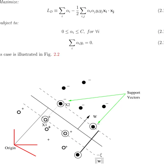
If the goal of the classification problem is to find a linear classifier for a non-separable training set (e.g., when data is noisy and the classes overlap), we can relax the constraints

2.2 and 2.3 by introducing a set of slack variables, ξi,i = 1, ..., l to allow for the possibility of examples violating the constraints yi(xi·w+b)≤1. Then we have:

w·x+b ≥+1−ξi f or yi = +1 (2.13)

w·x+b ≤ −1 +ξi f or yi =−1 (2.14)

ξi ≥0 f or ∀i (2.15)

In this case the margin is maximized, paying a penalty proportional to the cost C of con-straint violation, i.e.,CPl

(31)

The objective function to be minimized will be changed from ||w||2 _to _||_w_||2 ₊_C₍P

iξi) k_, whereC is a parameter to be chosen by the user and a largerC indicates to assign a higher penalty to errors. Here, for any positive integerk, the above optimization problem is a con-vex programming problem. However, if we choose k= 1, it is also a quadratic programming problem and furthermore the Lagrangian formulation in the Wolfe dual problem does not have the terms of ξi, which becomes:

Maximize: LD ≡ X i αi− 1 2 X i,j αiαjyiyjxi·xj (2.16) subject to: 0≤αi ≤C, f or∀i (2.17) X i αiyi = 0. (2.18)

This case is illustrated in Fig. 2.2

W Origin Support Vectors _ _ _ _ _ _ + + + + + + X1 X2 + −ξ ||w||

(32)

2.2.4

Nonlinear Support Vector Machines

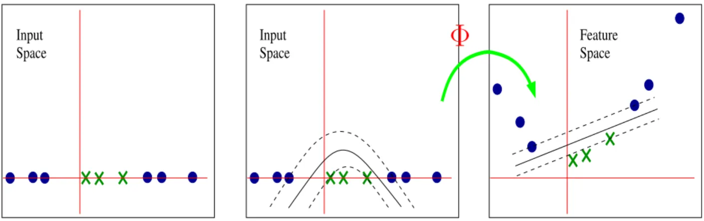
If the decision function is not a linear function of the data, the SVM works by mapping the training set into a higher dimensional feature space, Φ :_RD _→ _H_{, where the data becomes} linearly separable, using an appropriate kernel function K.

Input Space Input Space Feature Space

Φ

Figure 2.3: Example of mapping input spaces to feature spaces. The leftmost figure shows that the data set is in one dimension, which can not be separated by a linear hyperplane; the middle one shows that a non-linear hyperlane separates the data set with no errors. When mapped to a two-dimenion space, the data set is separated by a linear hyperlane in rightmost picture.

Since in the training procedure and in the decision function only dot products Φ(xi)· Φ(xj) need to be calculated, we only need to know what the dot product is, without need of even knowing what is the mapping function, Φ. Thus, we defineK, the so-called ”kernel function” such that K(xi,xj) = Φ(xi)·Φ(xj) and Eq. 2.16 transforms to

LD ≡ X i αi− 1 2 X i,j αiαjyiyjK(xi,xj) (2.19)

and the decision function changes to

fw,b(x) = sign( X i αiyiΦ(xi)·Φ(x) +b) = sign( X i αiyiK(xi,x) +b) (2.20)

(33)

there exists a mapping Φ and an expansion K(x,y) =X i

Φ(xi)Φ(yi) if and only if, for any

g(x) such that R g(x)2dxis finite, thenR K(x,y)g(x)g(y)dxdy≥0 Kernel Examples

1. Polynomial kernel:

K(x,y) = (x·y+ 1)p (2.21)

2. Gaussian radial basis function (RBF) kernel:

K(x,y) =e−||x−y)||/2σ2 (2.22)

For specific computational problems, the choice of a good kernel function is of importance. For alternative splicing, in previous workDSS05b _{use linear kernel with some basic biological}

features (we will state more about feature in next chapter) to get a good result. To achieve a more higher accuracy, in the workRSS05a_{, a kernel function, called as} _{shift weighted degree}

kernel, preforms well in predicting one specific isoform of alternative splicing. We use the LIBSVM implementation of SVM, available athttp://www.csie.ntu.edu.tw/~cjlin/ libsvm/, in our study.

2.2.5

Weighted Degree Kernel

The weighted degree kernel is a kind of measure for the similarity of pairwise sequence. The more similar two DNA sequences are, the higher the value of the kernel function is. The main idea is to count the number of occurrences of kmers appearing in both sequences s1 and s2, which share the same length L. The degree, denotedd, is defined as the maximum length of kmers matches between two sequences (i.e. k ∈ {1, ..., d}). The weights capture the idea that longer matches ofkmers contribute more significance to the kernel value. With respect to above ideas, the initial mathematical formulation introduced in the workSSP+₀₇

, given in 2.23 k(s_i,sj) = d X k=1 βk L−k+1 X l=1 I(uk,l(si) =uk,l(sj)) (2.23)

(34)

S2 S1

k(S1,S2) = w1 + w2 + w3 + w4+ w5

CCTCACTGCATACTCCCCGAGGAGTTAGG AGTCACTGAGTCGAGCCGATGGAATTAAA

Figure 2.4: Given two sequences of same length s1 and s2, the kernel value is the sum of all weights, each of which has a value depending on the length of matches, where longer matches contribute more value than smaller ones.

Here, the identity function I(term) is defined as: if term’s value equals true, then I = 1 otherwise I= 0. (uk,l(s) is the kmer starting from position l of the sequence s). Thus the inner summation corresponds to counting the matching occurrences ofkmer. Andβk is the weight coefficients assigned to each kmer, where mathematically βk = 2(d−k+ 1)/(d(d+ 1))SRS05_{. A note should be mentioned that} _β

k is a decreasing function of k (d is constant). This property of βk does not violate the assumption that longer matches contribute more strongly than smaller ones because long matches implies all summation of β of the shorter matches in 2.23. Furthermore, another trick for speeding up the kernel computation can be derived from the above observation: instead of calculating βk in 2.23 for each matches, the maximal length of kmer can be found first and an overall weight coefficient, so-called reward rb can be assigned to the maximal block. Figure 2.4 shows an example of how to compute the kernel value based on the two sequences. We give formulation of rb here.

rb =

(

(b(3db+ 3d−b2_{+ 1)}_/₃_d₍_d_{+ 1))} _for _b_≤_d

(b−d)(3−1/3) for b > d. (2.24) The WD kernel works well when the positions of two motifs are approximately same on two sequences. However, if one of the two motifs shifts one base in the sequence, the WD kernel will miss the matching. Therefore, in the workRSS05b _{the authors extend WD kernel}

in order to find such matching motifs with some-base shifts (Fig. 2.5illustrates the situation in which two motifs shift each other). The weighted degree kernel with shifts is defined as

(35)

S2 S1

k(S1,S2)

AGTCACTGAGTCGAGCCGATGGAATTAAA TCACTGCCCATACTCGCCGAGGAGTTAGG

Figure 2.5: Given two sequences of same length s1 and s2, the motifs have shifted each other in extent of several bases.

k(s_i,sj) = d X k=1 βk L−k+1 X l=1 γl S(l) X s=0 s+l≤L δSµk,l,s,si,sj (2.25) µk,l,s,si,sj =I(uk,l+s(si) = uk,l(sj)) +I(uk,l(si) = uk,l+s(sj)) (2.26)

where βk is the same as before; γl is the weights over the position l, SVM learns γl during the training process; δs = 1/(2(s+ 1)) is the weight assigned to shifts of distance s, where 0≤ s ≤S(l) subject to s+l ≤ L; andS(l) determines the shift range over the position l.

µk,l,s,si,sj is the extended function which compare each base in extent of shifts s.

2.3

Feature Selection Methods

Feature selection methods are used to select the most informative features with respect to a prediction or classification problem. Eliminating redundant or uninformative features helps to enhance the generalization capability of machine learning algorithms and to improve the model interpretability. In our study, we used two feature selection methods: (1) SVM feature importanceGWBV02 _{and (2) information gain}XJK01_{, to identify the most relevant}

features for distinguishing alternatively spliced exons from constitutive exons. The weight vectorw={|w0|,|w1|, ...,|wn|}(wheren is the dimension of the feature vector) determined by the SVM algorithm is used as a heuristic to identify important features using the SVM feature importance method.

The information gain criterion also provides a simple way to determine feature impor-tance. The information gain is the expected reduction in entropy caused by partitioning the

(36)

training examples into classes, according to a certain feature (where the entropy measures the impurity of a sample E of training examples). One can rank all features in the order of decreasing information gain and select relevant features conservativelyXJK01_{. A more robust}

way of identifying important features is to use a decision tree algorithm, which iteratively selects the feature with the highest information gain at each node of the tree. The features that are nodes in the final decision tree are considered to be more informative than the others.

(37)

Chapter 3

Data Set and Feature Construction

3.1

Data Set

3.1.1

Tribolium Castaneum

EST Data Set

The use of Tribolium castaneum for developing our methods. We have used data from the red flour beetle (Tribolium castaneum) for developing and testing algorithms and tools for identifying and analyzing alternative splicing in insects. Tribolium has become the second most powerful arthropod (after Drosophila) for genetic and molecular genetic studies. It has a genome sequence of approximately 200 Mbp in 10 chromosomes. The genome sequence is well established; the third assembled version was released recently by the Human Genome Research Center of Baylor College of Medicine. In addition, approximately 56,000 ESTs (most contributed by scientists from KSU and the USDA ARS GMPRC,) from five stage-specific or tissue-enriched cDNA libraries are available for Tribolium (namely, adult hindgut and Malpighian tubules; ovary; adult head; larval carcass, including fat body; and mixed-stage, whole larvae).Previous studies have shown the importance of alternative splicing in Tribolium. For instance, TcCHS1 chitin synthaseAHZ+04 and TcLac2 laccase-2 genesAMB+05 are found that these genes are alternatively spliced. They have compared the alternative splicing events for the same enzymes in several species.

With the EST data sets, we will design our experiments during which data sets will be cleaned, specifically, removing redundant ESTs. Then, we will align this cleaned EST data

(38)

sets to the genomic sequences of T. castaneum by using alignment tools. And then the algorithm of identifying AS events will be implemented

3.1.2

Alternative Splicing Data Set for Recognition

The data set used in our SVM prediction experiments contains alternatively spliced and constitutive exons in C.elegans. The methods to derive this data set has been introduced in section 2.1. It has been used in related workRSS05a _{and is available at} _http://www.

fml.tuebingen.mpg.de/raetsch/projects/RASE. A detailed description of how this data set was generated can be found in the wrokRSS05a_{. Briefly,} _C.elegans _{EST and full length}

cDNA sequences were aligned against theC.elegans genomic DNA to find the coordinates of exons and their flanking introns. After finding these coordinates, pairs of sequences which shared 3’ and 5’ boundaries of upstream and downstream exons were identified, such that one sequence contained an internal exon, while the other did not contain that exon. This procedure resulted in 487 alternatively spliced exons and 2531 constitutive exons. The final data set was split into 5 independent subsets of training and testing files for cross validation purposes.

3.2

Feature Construction

Six classes of features that affect alternative splicing are considered in our study: (1) pre-mRNA splicing motifs, specifically (1a) motifs derived from local sequences using MAST (MAST) and (1b) intronic regulatory splicing (IRS) motifs derived using comparative ge-nomics methods; (2) pre-RNA secondary structure related features, specifically (2a) the optimal folding energy (OFE) and (2b) a reduced motif set (RMS) obtained by taking the secondary structures into account; (3) exon splicing enhancers (ESE); (4) splice site strength (SSS); (5) GC-content (GCC) in introns; and (6) basic sequence features (BSF) used in the workRSS05a_{, specifically exon and flanking introns lengths and stop codon frames.}

(39)

3.2.1

Splicing Motifs

We used the MEMEBWML06 _{and MAST}BG98 _{tools available at} _{http://meme.sdsc.edu/}

meme/intro.html to detect motifs based on local sequences. MEME is a statistical tool for discovering unknownmotifs in a group of related DNA or protein sequences. Its underlying algorithm is an extension of the expectation maximization algorithm for fitting finite mixture modelsBE94_{. Optimal values for parameters such as the motif width and the number of motif}

occurrences are automatically found by MEME. Contrary to MEME, MAST is a tool for searching sequences with a group ofknownmotifs. A match score is calculated between each input sequence and each given motif. To use the MEME/MAST system, we first constructed local sequences by considering (-100, +100) bases around the donor sites (splice sites of upstream introns) and acceptor sites (splice sites of downstream introns) of the sequences in the original data set. Then, we ran MEME to obtain a list of 40 motifs (20 motifs for donor sites and 20 motifs for acceptor sites). MAST was used to search each sequence with these 40 motifs to obtain their location in each sequence and the corresponding p-values. Finally, we represented each sequence as a 40-dimensional feature vector. Each dimension corresponds to one of the 40 MEME motifs and indicates how many times that specific motif appears in the sequence.

In addition to motifs identified by MEME/MAST based on local sequences, we also considered intronic regulatory (IRM) motifs found by comparative genomics in Nema-todesKBSM+₀₆

. The basic idea of the comparative genomics procedure here is to identify alternatively spliced exons whose flanking introns exhibit high nucleotide conservation be-tween C.elegans and C.briggsae. Then, the most frequent pentamers and hexamers are extracted from the conserved introns. In our case, this procedure resulted in a list of 60 intronic regulatory motifs, 30 motifs for upstream introns and 30 motifs for downstream in-trons. For each sequence, we scanned the upstream intron with the upstream intronic motifs to find the number of occurrences of each motif. Each upstream intron is represented as a 30-dimensional vector, where each dimension indicates how many times the motif appears

(40)

in the sequence. The same approach is applied to the downstream introns of each exons. Altogether, this set of features is represented as a 60-dimensional vector.

3.2.2

Structural Konwledge

It is known that the splicing of exons can be enhanced or repressed by specific local pre-mRNA secondary structures around the splice sitesHZBS07,PYR02_. _{As shown in previous}

workHZBS07_{, motifs in single-stranded regions have more effect on the selection of splice}

sites than those in double-stranded regions. Following these ideas, we used the mfold

softwareMSZT99 _{available at} _{http://mfold.bioinfo.rpi.edu/} _{to predict the pre-mRNA}

folding (secondary structure formation) within a 100-base window around the acceptor and donor sites of each exon. Mfold parameters were chosen to prevent the formation of global double stranded base pairs. Thus, rather than folding the whole sequence, only local foldings were allowed. Two sub-classes of features related to the pre-mRNA secondary structure were considered in our study: (a) The Optimal Folding Energy, which roughly reflects the stability of the RNA folding; and (b) A reduced motif set derived, under the assumption that motifs on single stranded sequences are more effective than those on helices, from the set of MAST motifs by removing the motifs that are located on double stranded sequences with a probability greater than a threshold.

3.2.3

Splicing Regulators

Although splicing regulators have been identified in both introns and exons, exon splic-ing regulators (ESR) are more common and better characterized than intron splicsplic-ing reg-ulatorsCCK02. Exon splicing enhancers (ESE) affect the choice of splicing sites through recruiting arginine/serine dipeptide-rich (SR) proteins, which in turn bind other spliceo-somal components through protein-protein interactions. We adopted the approach in the workPMS07to search for specific ESEs in our data. Since recent studies show that ESEs tend to be less active outside the close vicinity of splice sitesPMS07, we used a 50-base window around the splice sites to search for ESEs. We also considered the following two assumptions

(41)

made in the RESCIE-ESE algorithmFYSB02,PMS07 _{in our search: (1) ESEs appear much more}

frequently in exons than in introns and (2) ESEs appear much more frequently in exons with weak splice sites than in exons with strong splice sites. The following two difference distribu-tions were computed in our study: (1){|fh

E−fIh||h∈all possible hexamers}, wherefEh is the frequency of a given hexamer h in exon regions within the 50-base windows, and fh

I is the frequency of a given hexamer hin intron regions; (2){|fh

W−fSh||h∈all possible hexamers}, where fh

W is the frequency of a given hexamer in exons with weak splice sites, and fSh is the frequency of a given hexamer in exons with strong splice sites. Given these two difference distributions, we set a threshold and obtained 77 hexamers with high frequency in the two difference distributions. We scan the exon of each sequence for these motifs and represent the sequence as a 77-dimensional vector, where each dimension indicates how many times the corresponding hexamer appears in the sequence.

3.2.4

Characteristics of Splicing Sites

Another feature we used in our study is given by the strength of the splice sites, as the strength has been shown to be informative for identifying alternatively spliced ex-onsTS03,WM06_{. More precisely, the strength is expected to be lower for alternatively spliced}

sites compared to constitutive splice sites. We used a position specific scoring-based ap-proachFH07_{to model the strength of splice sites, according to the following formula:} _score₌

X

i

logF(Xi)

F(X), where F(Xi) is the frequency of the nucleotide X at position i, and F(X) is the background frequency of the nucleotide X. As already known, in C.elegans the back-ground frequency is 66% AT. We extracted a range of (-3, +7) around donor sites (3 exon bases and 7 intron bases) and a range of (-26, +2) around acceptor sites (26 intron bases and 2 exon bases), and used the formula above to obtain scores for the strength of the acceptor and donor sites. The two ranges above are chosen to cover the main AG dinucleotides, which are bound by splicing factors around acceptor sites and the adjacent polypyrimidine tracts (PPT)WM06. Because the acceptor and donor sites can be seen as a pair, their scores are

(42)

summed together to obtain the overall splice site strength, which is represented as another feature.

3.2.5

Sequence Features

The GC content of a sequence is another feature correlated with the selection of splice sites. Alternatively spliced exons occur more frequently in GC-poor flanking sequencesTS03_{. We}

take into account this property by using a sliding window method to scan the GC content of each sequence within a range of (+100, -100) around donor and acceptor sites. The window size is set to 5, resulting in a 40-dimensional feature vector for each splice site. Each position indicates the ratio of GCs to the window size.

Last but not the least, sequence length has been shown to be a feature that can help distinguish alternatively spliced exons from constitutive exonsSSC+_04,DSS05b

. InRSS05a_{, a}

fea-ture vector consisting of upstream intron length, exon length, downstream intron length and the frame of the stop codon was constructed for each exon and its flanking introns. The length features were discretized into a logarithmically spaced vector consisting of 30 bins. The frame of the stop codons is represented using a 3D vector. In this study, we call this last set of features basic features.

(43)

Chapter 4

Experimental Results

4.1

EST-based Analysis of Alternative Splicing in

Tri-bolium

.

Pipeline for EST data analysis.

EST data analysis is an essential first step for all EST projects. Several EST data analysis pipelines are available as web-servers, e.g. ESTpassLHB+07_{, EGassembler}MNTK+06

and ESTexplorerNDGR07_{. However, they all have limitations, e.g., with respect to the amount}

of data that can be uploaded at once or the type and format of the annotations and statistics they provide. Given the increasing number of EST projects at KSU and the limitations of the publicly available pipelines, we have developed a local ArthropodEST pipeline for EST analysis (CPK+07 _{http://129.130.115.231/www_est/i3.html} _{within the KSU domain),}

using existing open source software tools. A prototype of browsable ArthropodEST database has been created and will be refined in the near future. Other tools for annotation will be added to the pipeline and customized statistics will be available.

Alternative splicing analysis in Tribolium.

We have taken the first steps towards the analysis of alternative splicing inTribolium. We have used the traditional approach to identifying alternative splicing, that is, aligning ESTs to the genome using GMAPWW05 _{and Exonerate}SB05_{. So far, we have analyzed GMAP}

(44)

analysis finds five types of alternative splicing events: alternative donor (AltD), alternative acceptor (AltA), alternative donor and acceptor (AltP), exon skipping (ExS) and intron retention (IntR). A total of 357 events are found in 213 Triboliumgenes based on our EST data. Our preliminary analysis (Table4.1) shows that intron retention is the most common type of alternative slicing event in Tribolium, followed by exon skipping.

Total AltD AltD% AltA AltA% AltP AltP% ExS ExS% IntR IntR%

357 45 13% 40 11% 27 7% 109 31% 136 38%

Table 4.1: Number of occurrences and percentage for each alternative splicing event.

ASpipe found 5809 expressed genes and estimated that approximately 4% of the genes in Triboliumundergo alternative splicing. Given that we have a relatively small number of ESTs, we expect that in reality many more Triboliumgenes are alternatively spliced. Cross-species EST to genome alignments and tiling arrays are expected to improve this initial estimate. The results of the ASpipe analysis have been displayed using ASviewWOBY08. The alternative events are marked in the viewer and are linked to the actual alignments, so that one could easily judge the correctness of the events found. Tools like ASview will prove invaluable for the manual analysis necessary to validate results of this bioinformatics approach. A preliminary examination of the results using ASview showed interesting splicing events. A more careful examination is needed to draw definite conclusions.

4.2

Alternative Splicing Prediction suing SVM

4.2.1

Motif Evaluation

The purpose of the motif evaluation in this section is to identify the splicing motifs that appear in several different sets, as those motifs are probably the most informative for alterna-tive splicing. To do that, we first compared the set of 40 motifs identified by MEME/MAST with the set of putative motifs found inRSS05a _{and the ISR motifs found in}KBSM+06_{. The}

(45)

Table 4.2: Intersection between MAST motifs, motifs found inRSS05a _{and ISR motifs found} inKBSM+₀₆

. MAST motifs 1-20 are around 5’ splice sites, while motifs 21-40 are around 3’ splice sites. ISR motifs are italicized.

MAST motifs E-value Contained Number

(Multilevel expression) hexamers

TTTTTTTTTCA 4.8e-046 tttttt mast2

GTGAGTTTTTT 4.6e-033 tttttt mast3

A

AAAAATTTTAAATTTTCAGG 3.9e-030 tttttt, atatat mast4

TT TTAAAATTT A tatata

ATTTTTCAAATTTTT 1.6e-026 tttttt mast6

T C T A C

GCCGGTGGAGCTGTCGTAGG 3.6e-026 gttgtc,catcgc mast9

A A CC CC GC GTAGC A gtgttg

AGCCGCCGAAGCCCTTGCCA 1.0e-018 gttgtc ,ccctgg mast14

CATT TA C AAAGCC GAG catcgc, cactgc

CAGCACCAACAGCACCACCA 1.4e-049 cagcag mast22

TC TG G TT G A

TTTTTTTTTTCAAAATTTTA 3.3e-038 tttaaa, aatttt mast23

(46)

two-level consensus sequences in Table 4.2. Upper-level bases have scores higher than or equal to the lower-level bases. A base is conserved if there is no lower-level base in its column. Eight motifs are found in all three sets compared, some of them (e.g., mast2 and mast3) being highly conserved among the C.elegans sequences in our data set.

Second, we compared the 77 ESE hexamers, found as described in Section 3.2.3., with two sets of candidate human and mouse ESE hexamers proposed inRES_{. Thirty two out}

of the 77 putative C.elegans ESE hexamers occur also in the human and mouse ESE sets, suggesting that the regulation of splicing, as well as the splicing process itself, are highly conserved in metazoans. Furthermore, a set of experimentally confirmed A. thaliana ESE ninemersPMS07 _{was used for comparison. The 32 conserved ESE hexamers are shown below;}

the A. thaliana ESE ninemers containing some of these hexamers are listed in brackets:

aatgga, aacaac,aagaag[GAAGAAGAA, GAGAAGAAG, TTGAAGAAG],aaggaa [GAAG-GAAGA],aaggag[AAAGGAGAT], attgga, atgatg, atggaa, atggat, acaaga, agaaga [GAA-GAAGAA, GAGAAGAAG], agaagc, tcatca, tgaaga, tgatga, tggaag, tggatc,caagaa [CAA-GAAACA], cagaag [GAGCAGAAG], cgacga, gaaagc, gaagaa [GAAGAAGAA, GAGAA-GAAG, GAAGAAAGA, TTGAAGAAG], gaagat [GAAGATGGA, GAAGATTGA], gaa-gag [GAAGAGAAA],gaagga[GAAGGAAGA], gatgat,gatgga[GAAGATGGA], gagaag, gaggag, ggaaga [GAAGGAAGA], ggagaa[ATGGAGAAA], ggagga.

It is worth mentioning that our study finds no intersection between the ISR motifs and the ESE motifs in C.elegans, suggesting that the two sets are functionally different.

4.2.2

Model Selection

The performance of a classifier depends on judicious choice of various parameters of the algorithm. For the SVM algorithm there are several inputs that can be varied: the cost of constraint violation C (e.g., C = 1), tolerance of the termination criterion (e.g., = 0.01), type of kernel used (e.g., linear, polynomial, radial or Gaussian), parameters of the kernel (e.g., the degree or coefficients of the polynomial kernel), etc.

(47)

Table 4.3: Results of alternatively spliced exons classification. All features, but ISR motifs, are included.

C Validation Score Test score

fp 1% AUC fp 1% AUC Split1 0.05 35.36% 86.99% 44.44% 89.32% Split2 0.05 36.50% 88.56% 46.92% 87.57% Split3 0.1 35.27% 86.91% 47.31% 88.59% Split4 0.01 37.56% 88.36% 26.88% 86.60% Split5 0.1 39.80% 88.03% 29.47% 86.98%

G. R¨atsch et al.RSS05ahave used basic features with several types of customized kernels, as well as an optimal sub-kernel weighting to learn SVM classifiers that differentiate between alternatively spliced and constitutive exons, and to identify motifs that can be used to interpret the results. In this section, we show that simple linear kernels can be used to obtain similar results if motifs are used as input features. In order to tune the costC, we use 5-fold cross-validation for each training set, with C ∈ {0.01,0.05,0.1,0.5,1,2}. We choose the value of C for which the area under curve (AUC) is maximized during the cross-validation. AUC is a global measurement which takes true positive ratio and false positive ratio into account. True positive ratio is the number of positively labeled examples classified by the algorithm as positive divided by the total number of positive examples. False positive ratio is the number of negatively labeled examples classified as positive divided by the number of negatively labeled examples.

Table 4.3 shows the results of classification of exons using all features described in Sec-tion 3, except conserved ISR motifs that need addiSec-tional informaSec-tion from closely related organisms to be determined. Table 4.4 shows the results when the conserved ISR motifs described in Section 3.2 are also included.

From Tables 4.3 and 4.4, we notice that on the average, the performance improves in terms of true positive rate at 1% false positive rate when ISR motifs are included, which means that ISR motifs conserved among several species contribute to better classification performance. Furthermore, the results are comparable and sometimes better than the results

(48)

Table 4.4: Results of alternatively spliced exons classification. All features, including ISR motifs are used.

C Validation Score Test score

fp 1% AUC fp 1% AUC Split1 0.05 32.45% 86.55% 56.48% 90.05% Split2 0.05 39.33% 88.32% 52.04% 89.04% Split3 0.1 37.56% 87.76% 38.71% 87.97% Split4 0.01 40.86% 89.02% 37.63% 84.42% Split5 0.1 36.48% 87.50% 35.79% 85.69%

obtained by G. R¨atsch et al.RSS05a_{. For example, when testing on the first data set we obtain}

a true positive rate of 56.48% at a fp rate of 1% and the AUC is 90.05%, thus improving the previous results of tp 51.85% at fp 1% and AUC 89.90%.

To evaluate how much the mixed features improve the performance of classification of alternatively spliced exons, we compared the AUC scores of classifiers trained on data sets with and without mixed features, respectively. Figure 4.1 shows the result of comparison between a data set with basic features only and a data set that includes the other features (except conserved ISR motifs).

Figure 4.2 shows a comparison of the AUC scores for each data set. It can be seen that the SVM classifiers using MAST motif features return higher AUC scores than those considering only basic sequence features.

In order to evaluate the effect of pre-mRNA secondary structure features on classification of alternatively spliced exons, we performed two experiments, one using data sets considering pre-mRNA secondary structure features obtained as described in Section 3.2 and the other using data sets without secondary structure features. Figure4.3 shows the results of the two experiments in which the classifiers were trained using 5-fold cross-validation with optimal cost parameters listed in Table 4.3. We can see the improvement obtained when considering secondary structure features.

(49)

0 0.1 0.2 0.3 0.4 0.5 0.6 0.7 0.8 0.9 1 0 0.2 0.