Periodic cycles of social outbursts of activity
H. Berestyckia, L. Rossi∗a, and N. Rodr´ıguezb
aEcole des Hautes Etudes en Sciences Sociales, PSL Research University, CNRS,
Centre d’Analyse et Math´ematiques Sociales, 190 - 198 avenue de France F-75244 Paris Cedex 13, France
bUNC Chapel Hill, Department of Mathematics, Phillips Hall, CB#3250, Chapel Hill, NC 27599-3250, USA
May 26, 2016
Abstract
We study the long-time behavior of a 2×2 continuous dynamical system with a time-periodic source term which is either of cooperative-type or activator-inhibitor type. This system was recently introduced in the literature [2] to model the dynamics of social outbursts and consists of an explicit field measuring the level of activity and an implicit field measuring theeffective
tension. The system can be used to represent a general type of phenomena in which one variable exhibits self-excitement once the other variable has reached a critical value. The time-periodic source term allows one to analyze the effect that periodic external shocks to the system play in the dynamics of the outburst of activity. For cooperative systems we prove that for small shocks the level of activity dies down whereas, as the intensity of the shocks increases, the level of activity converges to a positive periodic solution (excited cycle). We further show that in some cases there is multiplicity of excited cycles. We derive a subset of these results for the activator-inhibitor system.
1
Introduction
We study the convergence of trajectories of a 2×2 continuous dynamical system with a time-periodic source to limit cycles when the system is either cooperative or of activator-inhibitor type. The particular system we consider here is:
ut(t) =r(v(t))G(u(t))−ωu(t), (1a)
vt(t) =−h(u(t))v(t) +S(t), (1b)
satisfied for t > 0 and with non-negative initial data. This system has been introduced in [2] as a model for the dynamics of social outbursts. We provide a motivation to study this system in Section 1.1 by discussing a few examples of social phenomena that could be modeled by (1). The unknown u can represent, for example, the level of rioting activity and v measures the effective social tension in a system. The functionGis of KPP-type ([10]) and models self-excitement in the system. Specifically, we assume that Gis of classC3 and satisfies
G00<0, G(0) = 0, G(z)<0 forz large enough, r(0)G0(0)< ω < G0(0).
∗
However, we consider systems where the self-excitement in the system is negligible until the tension
v reaches a sufficiently large value; this switch mechanism is described by the function r which is a sigmoid function:
r(z) = 1
1 +e−β(z−a). (2)
The parameter β > 0 provides a measure of the transition slope between the relaxed state (non-excited) and the excited state. In other words, it provides a measure of how fast the transition is between a system that does not include the self-excitement and a system with the full-force of these factors. The critical tension, here denoted by a≥0, provides a measure of how large the tension needs to be before the switch (from relaxed to excited) is made. Note that in the limit β → ∞,
r approaches the step function 1[a,∞), in which case the self-excitement factors are in full-force as
soon as the tension is above the critical thresholda. We further assume that external events, which increase the tension v, occur with period T >0 and intensity A >0, leading to the source term
S(t) =A
∞
X
j=1
δ(t−T j), (3)
where δ is the Dirac mass at 0. Finally, the effect that the level of activityu has on the tensionv
is modeled by the term h(u), where
h: [0,∞)→(0,∞) is of class C1,
and it is either monotone increasing or decreasing 1. Note that the monotonicity of h determines whether (1) is of cooperative or activator-inhibitor type. For reason which will become apparent below we refer to (1) in the case when h is decreasing as a tension-enhancing system and in the case when his increasing as atension-inhibitive system. The case when his constant decouples the system. Considering the two cases allows us to differentiate between two different types of outbursts of activity from the modeling perspective. A typical example to have in mind is
h(u) = θ
(1 +u)p, θ >0, (4)
which is tension enhancing ifp >0 and tension inhibiting if p <0.
We treat the tension enhancing and the tension inhibitive systems separately as they lend them-selves to different analysis. In fact, in the former case we use heavily the fact that the system is monotone and thus a comparison principle is available. This property has been widely investigated in the literature and a complete theory of monotone systems is available. We recall some of its basic results in Section 1.2. However, exploiting the particular structure of the system, we will derive results which go beyond the ones provided by the general theory. The tension inhibitive case is no longer monotone, leading to some mathematical difficulties. To our knowledge, very few general results are known in such case.
Outline: We begin with a motivation from the application perspective, followed by a quick liter-ature overview on monotone systems and the statement of the main results of the paper. Section 2 is devoted to the existence and stability of the u ≡0 solution for both the tension enhancing and inhibitive systems. In Section 3 we focus on the tension enhancing case, where we are able to
1
characterize the existence and the bifurcation of excited cycles, as well as the long-time behavior of arbitrary solutions. We conclude the section with the simple case where his constant. In Section 4 we show the existence of excited cycles for the tension inhibitive system; we further derive some convergence results to excited cycles whenr is a step function and illustrate this numerically.
1.1 Motivation
System (1) models phenomena where there is an underlying potential field which accumulates energy and once this energy reaches a critical level then action is realized. This action in turn influences the field. This scenario occurs in multiple social phenomena where external factors lead to an increase in the potential field (we refer to it as the tension value) eventually leading to action. Then, internal factors maintain and increase the level of action for some period of time. We discuss briefly a number of applications which we have in mind.
System (1) was derived in [2] in the context of rioting activity. Riots and protests are complex social events that have been pervasive throughout history and which have been the subject of an intensive research activity– see for example [14, 11, 29, 1, 7, 22]. Much of this research has led to the belief that certain external events are responsible for initiating a period of rioting activity [17], these events are the so called triggering events. Of course, the issue is much more complex and, in addition to the triggering events, one must take into account long-established frustrations as they play a significant role in the intensity and duration of these social outbursts of activity [14]. This leads to an underlying dynamic tension field. Once the tension level reaches a critical value some researchers argue that there is contagion in the process of rioting activity thus leading to an escalation. There are many reason for this to be the case, for example the anonymity of a group may empower some people into action – see for example chapter 10 in [20].
The hypothesis of escalation has also been applied in the context of aggression, at the level of both dyads and groups. Indeed, some researchers have argued that hostile action from one party can be the impetus for even more hostile counteraction. This conjecture has been employed in the context of violent men [28], aggressive children [21], and violence in incarcerated young offenders [18]. System (1) is better suited in the context of wars between nations or groups of allied nations. Nation-states naturally fend for their interests and in many cases these nations have competing interests. This, as history has taught us, can easily lead to a crisis through a sequence of hostile events. If a certain threshold in the tension level between nation-states is surpassed the crisis can lead to military force. Once military force is initiated then self-reinforcement or escalation mechanism begins, where action begets more action. We refer to chapter 11 in [20] for an illustration of the escalation process during the First Kashmir crisis in 1947. See also [9] for a related model which includes the concept of reinforcement in conflicts.
inhibiting and tension enhancing cases.
In general terms, u(t) measures the level of activity and v(t) the effective tension in the sys-tem. For example, if the number of events follows a Poisson distribution, then u(t) represents the conditional intensity, which is evolving in time. The functionGmodels the endogenous factors, de-scribing the self-reinforcement mechanism. The function r is a monotone increasing function with values in (0,1) which can be thought of as a switch mechanism between arelaxed state (when the endogenous factors are not in effect) and anexcited state(when the endogenous factors are in effect), depending on the level of social tension. If there is no activity then there is a natural decay that is measured by the parameter ω >0.The triggering events are modeled as point-source terms and are included in S. Finally, the function h models the influence that the level of activity has on the decay of the tension: we consider both cases h decreasing andh increasing. This allows us to take into account two different modeling perspectives. The decreasing case leads to a tension enhancing
(cooperative system) where the level of activity relaxes the decay of the tension. This was the case explored in [2] and [3]. On the other hand, the casehincreasing leads to an activator-inhibitor type systems where the tension facilitates an increased level of activity, but this increased activity then leads to a certain level of fatigue. Thus, high levels of activity lead to a faster decay of the tension. We refer to this as thetension inhibitive case. This is an important and interesting regime as it has been observed in data from the 2005 French riots that the case p negative is a better suited model for the dynamics of those particular riots – refer to the paper in preparation [4]. This has also been observed in the London riots of 2011 [27].
An important aspect that remains to be studied for this system is the question of how various continuous external events, which we refer to as “shocks”, influence the qualitative behavior of activity. Clearly, there are many issues such as political decisions, the state of the economy, global issues, to name a few examples, are continuously affecting the tension in the system. These effects are random and extremely difficult to quantify exactly. Nevertheless, understanding the role that these types of events, which are occurring on a regular basis, play in the spatio-temporal dynamics of the level of activity is important.
A natural first step is to understand the effect of external events that occur on a periodic basis on a single site. Motivated by this consideration we analyze the case of periodic repeated shocks. Specifically, we study what happens when external events occur with a period T and intensity A. Numerical simulations performed in [2] illustrate the existence of periodic cycles for fixed intensityA
and sufficiently high frequency in the case whenhis decreasing. More precisely, for a fixed intensity, it was observed that if the period is above a threshold then the level of activity is “overdamped” -in the sense that the the solutions exhibit oscillations which quickly decay with time. On the other hand, for a sufficiently small period the solutions converge to a periodic cycle. The objective of the present paper is to prove this analytically as well as further understand these numerical finding for both the tension enhancing and tension inhibitive cases. From the mathematical point of view, the system behaves monotonically with respect to the intensity A, whereas in general there is no monotonicity in T. For this reason, in the present paper we mainly investigate how the dynamics changes whenA varies, and eventually apply the obtained results to describe its dependence on the length of the period T (c.f. Proposition 3.9 below), recovering the numerical observations of [2].
1.2 A quick review on monotone systems
System (1) is a continuous dynamical system with a periodic source term S(t). There is a vast literature on periodic dynamical systems. The theory is much more complex and rich than that of autonomous systems (i.e., with time-independent terms). The first questions that naturally arise are:
2. What is the long-time behavior of solutions to the Cauchy problem?
These two questions are clearly interconnected. Periodic solutions (cycles) are the natural extensions of fixed points for autonomous systems. Indeed, they are fixed points for the Poincar´e evolution operator of one period and one can hope that they attract all trajectories of the system. Unfor-tunately, it is well known since [23] that this property is not true for some autonomous systems. In fact, there are autonomous systems which exhibit a “chaotic behavior” or convergence to some “strange attractors”. For this reason a huge effort has been devoted to seeking suitable structural conditions which guarantee simple dynamical properties of the system, at least in low dimension. A different point of view consists in showing that complex trajectories, though possible, are not “generic”.
A structural condition which has been widely exploited is the monotonicity. This property is fulfilled by systems which are either cooperative or competitive. The work of Kamke [13] laid the foundation of the theory of monotone autonomous dynamical systems, which has been then systematically developed in the series of papers of Hirsch starting from [12]. We also refer to [25] for an extensive account of the theory. Theorem 2.3 in [12] states that solutions to 2×2 autonomous systems either diverge or converge to a fixed point. Massera partially extended this result to time-periodic monotone systems by considering the time-discrete dynamical system provided by the Poincar´e operator. The following two results are proved in [15]: for a single equation, any bounded solution converges to a cycle; for a 2×2 system, if all solutions exist for all times and there exists at least one bounded solution then there exists a cycle. However, in the latter case, no convergence of arbitrary solutions to the cycle is guaranteed. The lack of a convergence result shows a discrepancy between continuous and discrete dynamical systems, which has been further enlightened by Dancer and Hess in [8], who exhibited a 2×2 discrete system with non-constant solutions with period 2 (see also [26] for a system generated by a Poincar´e map). Because of this result, periodic solutions with a period which is a multiple of that of the system became the candidates as attractors of the system. It is shown in [19] that this is the case (for strictly monotone systems) at least generically.
1.3 Statement of the main results
The following notion is the central object of study of the paper.
Definition 1.1. We call a cycle a solution (u, v) to (1) which is periodic with period T. We say that the cycle is quiet ifu≡0, otherwise it is excited.
Of course, an excited cycle satisfiesu(t)>0 for all t≥0. We will see in the next section that the quiet cycle always exists and that it is stable if and only if the amplitude Aof the source term
Sis small enough. Actually, the overall dynamics of the system drastically depends on the value ofA.
Our results in the tension enhancing case, i.e. when h is decreasing, are summarized in the following.
Theorem 1.2(the tension enhancing case). Suppose thathis decreasing (in the weak sense). There exist then some thresholds 0< A∗≤A0 such that
• if A < A∗ then all solutions converge to the quiet cycle (as t→ ∞);
• if A∗ < A < A0 then, for any U > 0, there exists V ≥0 such that solutions with u(0) = U
converge to the quiet cycle if v(0)< V and to an excited cycle if v(0)≥V;
If the intensityAis below the thresholdA∗or above the thresholdA0then all nontrivial solutions
share the same type of limiting behavior. Depending on the parameters, and in particular on the amplitude of h0, the two thresholds may or may not coincide, as shown in Theorem 3.6 below. If they do then the second case of Theorem 1.2 is ruled out: the system is always monostable and a standard bifurcation takes place atA =A∗ =A0. On the other hand, if A∗< A0 then the system
is at least bistable in the regime A∗ < A < A0, where at least two excited cycles coexist as a result
of a turning point in the bifurcation diagram. The question of the exact number of excited cycles is left open.
It is worth noting that none of the properties stated in Theorem 1.2 follows from the general theory of monotone systems recalled in the previous section. In particular, the cycle provided by Massera [15] could be the quiet one (which always exists), leaving completely open the existence of excited cycles. On the other hand, [15] does not provide any information about the long-time behavior of solutions to the Cauchy problem. One could just infer from [19] that they “generically” converge to periodic solutions (not necessarily cycles) if h is strictly decreasing, which is weaker than the result of Theorem 1.2.
The tension inhibitive case is more complex to deal with due to the lack of monotonicity and, as a consequence, the results we obtain are less complete.
Theorem 1.3 (the tension inhibitive case). Suppose that h is increasing. There exists then a threshold A0>0 such that
• if A < A0 then all solutions converge to the quiet cycle;
• if A > A0 then any solution with u(0)>0 satisfies inft≥0u(t)>0, and moreover the system
admits an excited cycle.
When A > A0 we are not able to prove that any trajectory approaches an excited cycle, as
in the tension enhancing case, but only that they are bounded away from u ≡0. However, based on some numerical simulations, we conjecture that the convergence to excited cycles should hold. Surprisingly enough, the bifurcation scenario is simpler than in the previous case: as soon as the excited cycle appears (at A=A0) the quiet cycle becomes unstable.
With regards to the long-time behavior of solutions when A > A0, we are only able to obtain
partial results in the limiting case thatris the step function, which represents a discontinuous switch between the relaxed and the excited states. Namely, we find a threshold value ¯Acharacterizing the convergence to the cycle withu component identically equal to the maximal valueZ0, which is the unique positive zero ofz7→G(z)−ωz.
Theorem 1.4 (discontinuous switch). Suppose that h is increasing and that r = 1[a,∞). Then,
calling A¯:=a(eh(Z0)T −1), the following hold:
• if A <A¯then all solutions satisfy lim supt→∞u(t)< Z0;
• if A > A¯ then any solution with u(0) > 0 converges to the excited cycle with constant first
component Z0.
Gathering together Theorems 1.3 and 1.4 we infer that all solutions converge to cycles when either A < A0 (quiet cycle) or A > A¯ (excited cycle). In the intermediate case A0 < A < A¯ we
2
The quiet cycle
In this section we study solutions with theucomponent identically equal to 0, as well as the stability of the quiet cycle. The results are obtained regardless of the monotonicity ofh and thus they hold for both the tension enhancing and inhibiting cases. We begin with some preliminary properties.
The hypothesis on the self-excitement termG imply the existence of two constants 0< Z0 < Z
such that
Z is the unique positive zero of z7→G(z),
Z0 is the unique positive zero of z7→G(z)−ωz.
Then, since r <1, any solution to (1a) satisfies
∀t >0, u(t)<max{u(0), Z0}. (5)
Moreover, if u(0) 6= 0 then ut/u = G(u)/u−ω, whence, integrating and using the fact that by
concavity G(z)/z≤G0(0) for z >0, we get the following Gr¨onwall’s inequalities:
u(t)≤u(0)e(G0(0)−ω)t, u(0)≤Z =⇒ u(t)≥u(0)e−ωt. (6)
Let (u, v) be a solution to (1). Since
∀t∈(0, T), v(t) =v(0)e−´0th(u(s))ds,
the following implications hold:
v(T)< v(0) (resp. >) ⇐⇒ v(0)> A
1−e−´0Th(u(s))ds
(resp. <). (7)
Therefore (0, v) is a (quiet) cycle if and only ifv(0) =V, where
V := A
1−e−h(0)T. (8)
The quiet cycle always exists and it is a global attractor in the class of solutions satisfyingu(0) = 0. Indeed, the solution of equation (1b) is explicitly given by the formula
∀t∈[(n−1)T, nT), n∈N, v(t) =v(0)e−´0th(u(s))ds+A
n−1
X
j=1
e−
´t
jTh(u(s))ds, (9)
which, owing to (5), shows that v is bounded and, roughly speaking, it forgets the initial condition at exponential rate in time. If u(0) = 0 then u≡0 for all times and we find that
lim
n→∞v(nT) =Anlim→∞
n
X
j=1
e−(n−j)h(0)T =A
∞
X
k=0
e−kh(0)T =V ,
from which the convergence to the quiet cycle immediately follows by the continuous dependence of solutions with respect to initial data.
Lemma 2.1. There exists A0 >0 such that
if A < A0 then ∃ε, ε0 >0, σ∈(0,1),
(
u(0)≤ε
|v(0)−V| ≤ε0 =⇒
(
u(T)≤(1−σ)u(0)
|v(T)−V|< ε0 ,
if A > A0 then ∃ε, ε0 >0, σ∈(0,1),
(
0< u(0)≤ε
|v(0)−V| ≤ε0 =⇒
(
u(T)≥(1 +σ)u(0)
|v(T)−V|< ε0 ,
for any solution (u, v) to (1).
Proof. Fixε, ε0 >0 and let (u, v) be a solution to (1) with initial datum in [0, ε]×[V −ε0, V +ε0]. If u(0) = 0 then u ≡ 0 and the result immediately follows from equation (1b). Consider the case
u(0)6= 0. By (6) we have thatu=O(ε) in [0, T], where, here and in the rest of the proof, the term
O(·) refers to the limit as ε→0 orε0 →0 independently ofu(0) andv(0). We deduce that
∀t∈[0, T), v(t) =V e−´0th(u(s))ds=V e−
´t
0h(u(s))ds+O(ε0) =V e−h(0)t+O(ε) +O(ε0).
Hence, for t∈[0, T], plugging G(u) =u(G0(0) +O(ε)) in (1a) yields
ut/u=r(v)G0(0)−ω+O(ε) =r(V e−h(0)t)G0(0)−ω+O(ε) +O(ε0).
Integrating, we get
logu(T)
u (0) =G
0(0) ˆ T
0
r(V e−h(0)t)dt−ωT +O(ε) +O(ε0)
=G0(0)
ˆ T
0
r A e
−h(0)t
1−e−h(0)T
!
dt−ωT +O(ε) +O(ε0).
The strict monotonicity of r and the assumption
r(0)G0(0)< ω < G0(0) =G0(0)r(∞),
allow us to define A0 as the unique positive value for which T
0
r A0e
−h(0)t
1−e−h(0)T
!
dt= ω
G0(0), (10)
where ffl stands for the average integral, and to derive the following implications:
A < A0 (resp. > A0) =⇒ ∃σ∈(0,1),
u(T)
u(0) ≤1−σ (resp. ≥1 +σ) for ε, ε
0 small enough.
Concerning the second component, we have that
|v(T)−V|=|v(0)(e−h(0)T+O(ε))+A−V|=|(v(0)−V)e−h(0)T+v(0)O(ε)| ≤ε0e−h(0)T+(V+ε0)O(ε).
Hence, for fixed ε0, we have that |v(T)−V| < ε0 provided ε is small enough. This concludes the proof of the lemma.
Remark 1. In the limit caser =1[a,∞), direct computation shows that (10) reduces to
A0=e
ωh(0)T G0(0) a
1−e−h(0)T
Proposition 2.2. The quiet cycle is stable if A < A0 and unstable if A > A0, with A0 given
by (10), in the following sense:
(i) if A < A0 then, for any V ≥0, there exists U > 0 such that solutions with initial datum in
[0, U]×[0, V] converge to the quiet cycle ast→ ∞;
(ii) ifA > A0 then any solution(u, v) with u(0)>0 satisfiesinft≥0u(t)>0.
Proof. Note that any solution (u, v) to (1) is bounded due to (5) and (9). Using (9) and recalling the definition (8) of V we get
|v(nT)−V|=
v(0)e−
´nT
0 h(u(s))ds+A
n
X
j=1
e−
´nT
jT h(u(s))ds−A ∞
X
k=0
e−kT h(0)
≤(supv)e−γnT +A
n−1
X k=0 e− ´nT
(n−k)Th(u(s))ds−e−kT h(0)
+A ∞ X
k=n
e−kT h(0),
where γ is the minimum ofh on [0,supu]. Then, for anyε0 >0, there existsn0 ∈N, depending on
ε0, supv, supu,h,T and A, such that
v(n0T)−V
< A
n0−1
X k=0 e−
´n0T
(n0−k)Th(u(s))ds−e−kT h(0)
+ ε 0 2.
Since the first term of the right-hand side vanishes if u ≡ 0 on [0, n0T], using the first property in (6) we can find η >0, depending on the same terms as n0, for which there holds
u(0)≤η =⇒ |v(n0T)−V|< ε0. (11)
Case (i) A < A0.
Let ε, ε0, σ be given by the first case of Lemma 2.1. Take V ≥0. It follows from (5) and (9) that the family of solutions emerging from initial data in [0,1]×[0, V] is uniformly bounded inL∞(R+).
There exist thenn0 ∈Nandη >0 such that any (u, v) in this family satisfies (11). Hence, solutions emerging from [0, U]×[0, V], with U = min{η,1}, satisfy |v(n0T) −V| < ε0. Moreover, up to reducing U,u(n0T)< εand therefore they fulfill the hypotheses of Lemma 2.1 at timen0T instead of time 0. Applying recursively Lemma 2.1 yields
∀n∈N, u((n0+n)T)≤(1−σ)nu(n0T), |v((n0+n)T)−V|< ε0.
As a consequence, u(nT) → 0 as n→ ∞, hence u(t) → 0 ast → ∞, and then (9) readily implies that (u, v) converges to the quiet cycle.
Case (ii) A > A0.
Letε, ε0 be from the second case of Lemma 2.1. Consider a solution (u, v) withu(0)>0. Letn0∈N
and η >0 be such that the implication (11) holds. We claim that
∀n∈N, u(nT)≥µ e−ω(n 0+1)T
, with µ:= min{u(0), Z, η, ε}, (12)
which would conclude the proof of the theorem. Suppose that (12) fails for some n=m+ 1∈N. Then, if there exists τ <(m+ 1)T such thatu(τ) =µ, the second property in (6) yields
whence τ < (m−n0)T. This shows that u((m−n0)T) < µ (and also that m > n0) and thus the function u(·+ (m−n0)T) satisfies the hypothesis in (11), from which, recalling that n0, η
depend on the solution only through supu, supv, we deduce that|v(mT)−V|< ε0. Sinceu(mT)≤
u((m+1)T)eωT < µ≤εalways by (6), we can apply Lemma 2.1 and infer thatu((m+1)T)> u(mT),
that is, (12) fails for n=m too. In other words, if (12) holds for somen∈Nthen it holds true for
n+ 1. We deduce that it holds for alln∈N.
3
The tension enhancing system
This section is devoted to the study of the tension enhancing case, that is, h is assumed to be decreasing (in the weak sense). The key property of the tension enhancing system is that it is monotone - or cooperative, with the terminology of [12]. This is expressed by the following variant of the classical comparison principle of Kamke [13].
Proposition 3.1 (Monotonicity). Let (u1, v1) and (u2, v2) be two solutions such that u1(0) ≤
u2(0) ≤ Z and v1(0) ≤ v2(0). Then u1 ≤ u2 and v1 ≤ v2 for all positive times, with strict
inequalities if v1(0)< v2(0).
Proof. Note first that equation (1a), together withG(Z) = 0, yieldu1, u2≤Z for all times. Assume
by contradiction that u1 > u2 orv1 > v2 at some moment. Define
τ := inf{t >0 : u1(t)> u2(t) or v1(t)> v2(t)}.
In particular,u1 ≤u2 andv1 ≤v2 in [0, τ], and equality holds att=τ in at least one case. Actually,
it holds in exactly one case because otherwise (u1, v1)≡(u2, v2) for all times by uniqueness of the
Cauchy problem. We just treat the case u1(τ) =u2(τ), the other one being similar. In such case
v1 < v2 in [τ, τ+k) for ksmall enough. By the monotonicity of r (or of−h in the other case), the
functionu:=u2−u1 satisfies
∀t∈[τ, τ+k], ut≥
r(v1)
G(u2)−G(u1)
u2−u1
−ω
u.
Therefore, Gr¨onwall’s inequality yields u ≥ 0 in [τ, τ +k], which entails a contradiction with the definition of τ. This shows thatu1≤u2 andv1 ≤v2 for all times.
Suppose now that v1(0) < v2(0). Then, by (1) and the strict monotonicity of r, there exists
k >0 such that both u1 < u2 and v1< v2 in (0, k). Applying Gr¨onwall’s inequality to u2−u1 and
v2−v1 in intervals of the type [0, τ] one readily obtains u1 < u2 and v1< v2 for all t >0.
In view of the above comparison principle, solutions are increasing with respect to the parameter
Afor allt >0. This is the reason why we useAas the varying parameter in the bifurcation analysis of the system.
3.1 Existence and non-existence of excited cycles
We investigate the global stability of the quiet cycle as well as the existence of excited cycles, in the sense of Definition 1.1. We use a discrete-time dynamical system approach, introducing the Poincar´eT-step evolution operator
where (u, v) is the solution to (1) emerging from (U, V). Excited cycles emerge from positive fixed points forE. Our main result states the existence of a critical thresholdA∗separating the existence and non-existence of excited states; in addition, forA < A∗, the quiet cycle is a global attractor for the system. The proof relies on the following key auxiliary result.
Proposition 3.2. Let (u, v) be a solution to (1). Then, there exists a cycle emerging from some
(U, V) satisfying
U ≥lim sup
n→∞ u(nT), V
≥lim sup
n→∞ v(nT).
Proof. Consider a solution (u, v) to (1) Recall that (u, v) is bounded owing to (5) and (9). Call
ˆ
U := lim sup
n→∞
u(nT), Vˆ := lim sup
n→∞
v(nT).
For ε >0, let n∈Nbe such that
u(nT)≥Uˆ −ε, u((n−1)T)≤Uˆ +ε, v((n−1)T)≤Vˆ +ε.
Since
E u((n−1)T), v((n−1)T)
= u(nT), v(nT)
∈[ ˆU −ε,∞)×R+,
we deduce from the comparison principle, Proposition 3.1, that
E( ˆU+ε,Vˆ +ε)∈[ ˆU −ε,∞)×R+.
As a consequence, by the arbitrariness ofε and the continuity ofE, we get
E( ˆU ,Vˆ)∈[ ˆU ,∞)×R+.
With analogous arguments one derives the inclusion for the second component, whence E( ˆU ,Vˆ) ∈
[ ˆU ,∞)×[ ˆV ,∞).
With this property in hand, the existence of the desired cycle is a consequence of the following general fact:
E(U, V)∈[U,∞)×[V,∞) =⇒ {En(U, V)} is componentwise increasing, (13)
which is readily obtained by induction on n, using the comparison principle. It follows that the sequence{En( ˆU ,Vˆ)}is componentwise increasing (and bounded) and therefore it converges to some
pair (U, V) ∈[ ˆU ,∞)×[ ˆV ,∞). By the continuity of the solutions with respect to initial data, we eventually infer that (U, V) is the initial datum of a cycle.
Let us mention an alternative way to conclude the proof of Proposition 3.2: once one knows that [ ˆU ,∞)×[ ˆV ,∞) is invariant under the mapping E, it is easy to find ˜U , V˜ such that the same is true for [ ˆU ,U˜]×[ ˆV ,V˜]; then one applies Brouwer’s fixed point theorem. A more involved version of this argument will be used to derive the existence of excited cycles in the tension inhibitive case, where the comparison principle is not available. Property (13), together with the specular one:
E(U, V)∈[0, U]×[0, V] =⇒ {En(U, V)}is componentwise decreasing, (14)
Proposition 3.3. There exists a threshold
A∗ ∈h 1−e−h(Z0)Tr−1(ω/G0(0)), A0
i
(15)
such that
(i) ifA < A∗ then all solutions converge to the quiet cycle as t→ ∞;
(ii) ifA > A∗ then the system admits at least one excited cycle.
Proof. Let us call
A:={A : the system admits an excited cycle}.
Step 1. A∗ := infA satisfies (15).
LetA > A0. Consider a solution (u, v) to (1) withu(0)>0. By Proposition 2.2 part (ii), infu >0
and therefore the cycle provided by Proposition 3.2 is excited. This shows A∗ ≤ A0. Conversely,
consider an arbitrary A ∈ A and let (u, v) be an associated excited cycle. Since u(T) = u(0), (5) yields u(0) < Z0 and then u < Z0 for all times. Combining this with (7) and the fact that h is decreasing, we deduce
u(0)< Z0, v(0)≤ A
1−e−h(Z0)T. (16)
Moreover, since u cannot be strictly monotone in [0, T], there exists t∈[0, T] such that
ωu(t) =r(v(t))G(u(t))≤r(v(0))G0(0)u(t),
which, together with the second inequality in (16), provides the lower bound for Ain (15).
Step 2. Ais a half-line.
Let (u, v) be an excited cycle associated with a givenA∈ A, with initial datum (U, V). Take ˜A > A
and let (˜u,˜v) be the solution to (1) with A replaced by ˜A, also emerging from (U, V). Clearly,
˜
u(T) =u(T) =U, v˜(T) =v(T) + ˜A−A > V.
Namely, callingE theT-step Poincar´e operator associated with ˜A, there holds E(U, V)⊂[U,∞)×
(V,∞), and therefore, by (13), the sequence{En(U, V)}, which is bounded due to Proposition 3.2,
is componentwise increasing. Its limit ( ˆU ,Vˆ) ∈ [U,∞)×(V,∞) is thus the initial datum of an excited cycle, i.e., ˜A∈ A.
Step 3. Statement (i).
Let Abe such that there exists a solution (u, v) satisfying
lim sup
n→∞
u(nT)>0.
Then, Proposition 3.2 implies the existence of an excited cycle, i.e., A ≥ A∗. It follows that, if
A < A∗, any solution (u, v) satisfies u(nT) → 0 as n → ∞, which readily implies that (u, v)
converges to the quiet cycle as t→ ∞.
Proposition 3.4. There exists a cycle(u, v) such that any solution (u, v) to (1)satisfies
lim sup
t→∞
(u(t)−u(t))≤0, lim sup
t→∞
(v(t)−v(t))≤0.
Proof. Let (˜u,v˜) be the solution to (1) with initial datum ( ˜U ,V˜) given by
˜
U := sup{u(0) : (u, v) is a cycle}, V˜ := sup{v(0) : (u, v) is a cycle}.
We have seen that any cycle satisfies (16) and thus the above quantities are finite. By comparison, for any cycle (u, v), there holds
∀n∈N, u˜(nT)≥u(nT) =u(0), v˜(nT)≥v(nT) =v(0),
whence, taking the sup among all cycles,
∀n∈N, u˜(nT)≥U ,˜ v˜(nT)≥V .˜ (17)
Next, by Proposition 3.2, there exists a cycle (u, v) satisfying
u(0)≥lim sup
n→∞ u˜(nT), v(0)
≥lim sup
n→∞ ˜v(nT).
On one hand, u(0)≥U˜,v(0)≥V˜ by (17), on the other, the definition of ˜U and ˜V yields ˜U ≥u(0), ˜
V ≥v(0). This means that the cycle (u, v) emerges from ( ˜U ,V˜).
Consider now an arbitrary solution (u, v) to (1). Applying again Proposition 3.2 we find a cycle emerging from an initial datum (U, V) satisfying
U ≥lim sup
n→∞
u(nT), V ≥lim sup
n→∞
v(nT).
Hence,U ≤U˜,V ≤V˜, which entails
lim sup
n→∞ u(nT)
−u(nT)= lim sup
n→∞ u(nT)
−U˜ ≤U −U˜ ≤0,
lim sup
n→∞
v(nT)−v(nT)
= lim sup
n→∞
v(nT)−V˜ ≤V −V˜ ≤0.
The first statement of the proposition follows from these inequalities by using the continuous de-pendence with respect to initial data and the comparison principle.
Let us prove the second statement of the proposition. Consider the above cycle (u, v) associated with a given A >0. Take ˜A > A. We have seen in the Step 2 of the proof of Proposition 3.3 that there is a cycle (ˆu,ˆv) for (1) withA replaced by ˜A, satisfying ˆu(0)≥u(0), ˆv(0)> v(0). Hence, by Proposition 3.1,
∀t∈[0, T), uˆ(t)≥u(t), vˆ(t)> v(t),
that gives the desired monotonicity property. Finally, let{(un, vn)}be the cycles constructed above
for a sequence{An}of values ofAconverging to someA >0. By the monotonicity property derived
before, {un} and {vn} have the same monotonicity behavior as {An} and then to prove the result we can restrict to the case where An & A. We have that {(un, vn)} converges pointwise to some
function (u, v). By continuity with respect to initial data, (u, v) is a solution (cycle) to (1) with the value A and the convergence holds uniformly fort≥0. Thus, the cycle (u, v) associated with
A satisfiesu≥u,v≥v. The proof of the proposition is thereby complete.
3.2 The branch of excited cycles
We now investigate the properties of the branch of excited cycles as a function of Aand of the first component of the initial datum of the cycle. We will show its bifurcation from the quiet cycle, with the possibility of a turning point and the coexistence of multiple excited cycles. The latter occurs when −h0(0) is sufficiently large (how large is made concrete in Theorem 3.6).
We know from (5) that any cycle satisfies u(0) < Z0. Take U ∈ (0, Z0). We claim that there exists a uniqueV >0 such that the solution (u, v) emerging from (U, V) satisfiesu(T) =U. First, by Proposition 3.1, u(T) is a strictly increasing and continuous function of V ≥ 0. Next, on the one hand, if V = 0 then
∀t∈(0, T), ut=r(0)G(u)−ωu≤(r(0)G0(0)−ω)u <0
by hypothesis, whence u(T)< u(0). On the other hand, ifV is large enough then the same is true forv in [0, T], from which we deduce
∀ε >0, ∃V >0, ∀t∈[0, T], ut=r(v)G(u)−ωu≥(1−ε)G(u)−ωu. (18)
Since G(U)−ωU > 0 because U < Z0, we can choose ε small enough in such a way that (1−
ε)G(U)−ωU >0, which implies that u(t) > U fort∈(0, T]. We let VU denote this unique value
for which the solution (u, v) emerging from (U, VU) satisfies u(T) =U. By (7), such solution is a
cycle if and only ifA=C(U), where
C(U) :=VU
1−e−
´T
0 h(u(s))ds
.
This shows that the branch of excited cycles can be parametrized by U. This is stated rigorously in the next result, together with the fact that the branch bifurcates from the quiet cycles U = 0 at
A=A0.
Proposition 3.5. System (1) admits an excited cycle with initial datum (U, V) if and only if
U ∈(0, Z0) and V =VU, A=C(U) (uniquely determined by U).
Moreover, the functionC is continuous and satisfies
lim
U→0C(U) =A0, Ulim→Z0C(U) =∞.
Proof. It only remains to prove the second part of the proposition. For givenU ∈(0, Z0), let (u, v) be the solution emerging from (U, V). The continuity ofC follows from its definition, owing to the continuity of VU and uwith respect to U.
For the limit asU →Z0, we first remark that the definition of Z0 and the fact thatr <1 imply that VU → ∞ asU %Z0. It then follows thatC(U)→ ∞ asU →Z0.
Let us derive the limit as U → 0. As U → 0, the VU stay bounded, because otherwise (18)
and G0(0)> ω would readily implyut>0 in [0, T], which contradicts the definition ofVU. Hence,
the same holds true for C(U) by definition. Assume by contradiction that (up to subsequences)
C(U)→A6=A0 asU →0. We compute
lim
U→0VU = limU→0
C(U)
1−e−´0Th(u(s))ds
= A
1−e−h(0)T.
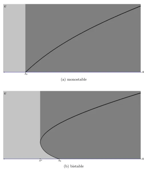
The infimum of C is the quantity A∗ in Proposition 3.3. If A∗ < A0 then it is a minimum,
and thus for A∈(A∗, A0) the system admits at least two excited cycles. We show below that this
situation can actually occur, through the analysis of the second order expansion of the system. The two different cases are illustrated in Figures 1a, 1b. The black curve is the graph of U 7→ C(U).
(a) monostable
(b) bistable
Figure 1: the curve A = C(U); (a) monostable regime when |h0| 1, (b) bistable regime for
A∈(A∗, A0) when|h0| 1.
Theorem 3.6. The following different scenarios occur when, respectively,sup|h0|is small or|h0(0)|
is large (depending on the other terms of the system):
(a) A∗ =A0 and, asA&A0, the maximal cycle associated with A converges to the quiet cycle;
(b) A∗< A0 and the system admits an excited cycle for A=A∗ and at least two excited cycles for
A∈(A∗, A0).
Proof.
(a) TakeA∈(A0, A0+ 1) and let (u, v) be an excited cycle with an initial datum (U, V), which
exists by Proposition 3.3. Recall that u < Z0 < Z for all times. We deduce from (6) that
where κ, κdepend onT,G0(0), ω. Then, from v(T) =V, we obtain
V = A
1−e−´0Th(u)
≤ A
1−e−(h(0)−sup|h0|κU)T.
If sup|h0| is small enough, depending on T, G0(0), ω, Z0 and h(0), there holds that sup|h0|κU ≤ h(0)/2 and therefore V ≤V + sup|h0|O(U), where V is given by (8) and O depends on T,G0(0),
ω,h(0), A. Hence,
∀t∈[0, T), v(t)≤(V + sup|h0|O(U))e−h(0)t+sup|h0|κU ≤V e−h(0)t+ sup|h0|O(U),
whereO depends on the same terms as before. Then from (1a), using the above inequality together withG(u)/u≤G0(0)−Γu≤G0(0)−ΓκU, where Γ :=−max[0,Z0]G00/2>0, we derive fort∈(0, T),
ut/u≤r V e−h(0)t+ sup|h0|O(U)
G(u)/u−ω
≤r V e−h(0)t
(G0(0)−ΓκU)−ω+ sup|h0|O(U),
with O also depending onr. Integrating we get
0 = logu(T)
u(0) ≤G
0(0) ˆ T
0
r V e−h(0)t
dt−r V e−h(0)T
ΓκT U −ωT + sup|h0|O(U).
Thus,
h
r V e−h(0)TΓκT −sup|h0|O(1)
i
U ≤G0(0)
ˆ T
0
r V e−h(0)tdt−ωT,
which tends to 0 asA→A0by the definition (10) ofA0. Sincer(V e−h(0)T)→r(A0/(eh(0)T−1))>0
as A→ A0, if sup|h0| is small enough, we necessarily have that U →0. This applies in particular
to the maximal cycle (u, v), showing that, as A & A0, it converges to the quiet cycle, that is,
u→0. Therefore, by the monotonicity provided by Proposition 3.4, the maximal cycle is quiet for all A≤A0, whence A∗ =A0.
(b) Let (u, v) be an excited cycle for system (1) with an initial datum (U, V). We know from Proposition 3.5 that U ∈(0, Z0),V =VU and A=C(U). Suppose that
C(U)≥A0.
It follows from (1a) that κU < u < κU in [0, T], where, here and in the sequel, κ, κ will denote some generic positive constants independent of U,h0(0) and G00(0), whose value will change during the proof. Then, by (7) and the fact that h is decreasing,
VU =
C(U)
1−e−´0Th(u(s))ds
≥ A0
1−e−h(κU)T,
whence, noticing thatz7→A0/(1−e−z) is decreasing,
VU ≥
A0
1−e−h(0)T −κh
0(0)U−κU2.
We infer that
∀t∈[0, T), v(t) =VUe− ´t
0h(u)≥
A0
1−e−h(0)T −κh
0(0)U −κU2
Let us further suppose that
U ≤ |h0(0)|−1. (19)
Plugging the inequality for v into (1a) and usingG(u)/u≥G0(0)−G00(0)u−κu2 yields
ut/u=r(v)G(u)/u−ω
≥G0(0)r A0e
−h(0)t
1−e−h(0)T
!
−G0(0)κh0(0)U e−h(0)T −κU2+κG00(0)U−ω
=G0(0)r A0e
−h(0)t
1−e−h(0)T
!
−ω+ −κh0(0) +κG00(0)−κUU.
As a consequence, by the definition (10) of A0,
0 = logu(T)
u(0) =
ˆ T
0
ut/u≥ −κh0(0) +κG00(0)−κU
U.
This shows that, if κh0(0)< κG00(0), thenU cannot be arbitrarily small. In other words, in such case, C(U) < A0 for U small enough, whence Proposition 3.5 implies A∗ = minC < A0 and the
multiplicity of excited cycles for A∈(A∗, A0).
We remark that the existence of at least three cycles (one quiet and two excited) stated in Theorem 3.6 (b) is in accordance with theorder interval trichotomy(for strictly monotone systems) from [16, 8].
3.3 Asymptotic convergence to cycles
In this subsection we prove that all trajectories eventually converge to a cycle. This is a strong and quite unexpected property. We indeed know from the literature that much more complicated trajectories cannot be excluded in principle. The general theory only tells us that for “most of the initial data” the solution converges to a periodic solution with period equal to some multiple of T
(thus not necessarily a cycle). Here we derive a much stronger result. The proof is based on an accurate analysis of the admissible dynamics for (1) which, unlike the previous arguments, exploits the peculiar structure of the system beyond the simple monotonicity. For this reason, we decide to state it after having proved independently the other results, that we expect to hold true in more general situations where the comparison principle holds.
We start with a preliminary observation.
Lemma 3.7. Let (u, v) be a solution to (1). Then, u is either constant or strictly monotone in
[0, T], or there existst such that u is strictly increasing in [0, t) and strictly decreasing in (t, T].
Proof. If v(0) = 0 then v ≡ 0 and therefore u is either constantly equal to 0 or to the zero of
r(0)G(z)−ωz, or it is strictly monotone. Suppose that v(0) > 0, whence v is strictly decreasing in [0, T). Assume that u(0)6= 0 (whence u 6= 0 for all times) and that there exists t∈(0, T) such that ut(t) = 0. It follows that r(v(t))G(u(t))−ωu(t) = 0 withG(u(t))>0. Calling M :=u(t), we
derive
∀t∈(t, T), (u−M)t=r(v)G(u)−ωu=r(v)G(u)−r(v(t))G(M)−ω(u−M)
< r(v)[G(u)−G(M)]−ω(u−M)
=
r(v)G(u)−G(M)
u−M −ω
which is a linear differential inequality foru−M with a continuous coefficient (GisC1). Gr¨onwall’s
inequality eventually implies that u < M in (t, T). Analogously, one sees that u < M in (0, t) too. We have proved that any stationary point in (0, T) is of local strict maximum, and thus the statement of the lemma.
Theorem 3.8. Any solution to (1) approaches a cycle (quiet or excited) as t→ ∞.
Proof. We prove the statement showing that for any solution (u, v) the sequence {(u(nT), v(nT))}
is definitely componentwise monotone. Then, being bounded thanks to (5) and (9), it converges to some pair, which is the initial datum of a cycle. The conclusion of the theorem eventually follows from the continuity with respect to initial data.
As usual, we let E denote the T-step Poincar´e operator. We say that a point (U, V) ∈[0,∞)2 satisfies
NE if E(U, V)∈[U,∞)×[V,∞), SW if E(U, V)∈[0, U]×[0, V],
NW if E(U, V)∈[0, U)×(V,∞), SE if E(U, V)∈(U,∞)×[0, V).
Note that any point in [0,∞)2 satisfies just one of the above four properties, excepted for the fixed points for E which fulfill simultaneously NE and SW. It follows from (13) and (14) that if (U, V) satisfies NE or SW respectively, then so does the whole sequence {En(U, V)}.
The key of the proof is to show that if (U, V) satisfies NW then E(U, V) does not satisfy SE. Suppose by contradiction that the solution (u, v) emerging from some (U, V) satisfies
(
u(T)< U
v(T)> V ,
(
u(2T)> u(T)
v(2T)< v(T) .
Throughout the proof, v(nT−), n ∈ N, stands for the limit of v(t) as t → nT− (recall that v is discontinuous on TN). Since
v(2T−) =v(2T)−A < v(T)−A=v(T−)< V < v(T),
there existsτ ∈(T,2T) such thatv(τ) =V. We distinguish two possible situations.
Case u(τ)< U.
From the fact that v(τ) = V > v(T−) > v(2T−), we deduce the existence of another time τ0 ∈
(τ,2T) such thatv(τ0) =v(T−). Because the trajectories
{(u(t), v(t)) : t∈[τ,2T)}, {(u(t), v(t)) : t∈[0, T)}
cannot intersect by uniqueness of the Cauchy problem, we necessarily have that u(τ0) < u(T). Hence, by Lemma 3.7, u < u(T) in (τ0,2T], in contradiction with u(2T) > u(T). This case is therefore ruled out.
Case u(τ)≥U.
Proposition 3.1, applied with (u1, v1) = (u, v) and (u2, v2)(t) = (u, v)(t+τ) fort∈(0,2T −τ) (in
which v1,v2 do not jump), implies that
v(2T−)≥v(2T−τ).
Thus, since v(2T −τ) > v(T−) because 2T −τ < T, we infer that v(2T−) > v(T−), that is,
v(2T)> v(T), which is a contradiction.
NW
SW SE
NE
We eventually infer that, for any solution (u, v) to (1), the sequence {(u(nT), v(nT))} either fulfills definitely one of the properties NE, SW, NW, or it always satisfies SE. Thus, in any case, it is definitely componentwise monotone. This concludes the proof of the theorem.
3.4 Basins of attraction
Gathering together all previous results we can conclude the analysis in the tension enhancing case.
Proof of Theorem 1.2. We know from Theorem 3.8 that any solution converges to a limit cycle, which can be quiet or excited. The statement of the theorem in the caseA < A∗ is Proposition 3.3 part (i). IfA > A0 then the limit cycle is necessarily excited due to Proposition 2.2 part (ii).
It remains the caseA∗< A < A0. FixU >0 and define
VU := inf{V ≥0 : the solution emerging from (U, V) converges to the excited cycle}.
Let (u, v) be the solution emerging from (U, V), with V to be chosen, and let ( ˜U ,V˜) be the initial datum of the excited cycle provided by Proposition 3.3 part (ii). We know from (5) that ˜U < Z0. Note that the solution of ut=G(u)−ωu with initial datumU converges toZ0 ast→ ∞and thus
it is larger than ˜U att=nT fornlarge enough. Therefore, since
∀t∈[0, nT], v(t)≥V e−h(0)nT,
for large V we have that r(v) ∼1 in [0, nT], whence u(nT) >U˜. Moreover, up to increasing V if need be,v(nT)>V˜. It follows by comparison that (u, v) is componentwise greater than the excited cycle for t ≥ nT, and thus its limit cycle is excited. This shows that the set in the definition of
VU is nonempty. The comparison principle also implies that it is a right half-line. Assume now by way of contradiction that the limit cycle of the solution (u, v) emerging from (U, VU) is quiet. Let
ˆ
U > 0 be the quantity U given by Proposition 2.2 part (i) associated with V =V + 1, where, we
recall, (0, V) is the initial datum of the quiet cycle. There exists n∈N such that u(nT) <Uˆ and
v(nT) < V + 1. By continuity with respect to initial data, the same property holds true for the
solution emerging from (U, VU+ε) for ε >0 small enough. Then Proposition 2.2 part (i) ensures that such solution converges to the quiet cycle, contradicting the definition of VU. This concludes the proof of the theorem.
Remark 2. We know from Theorem 1.2 that if A > A0 then any solution (u, v) with u(0) > 0
approaches some excited cycle (˜u,v˜) ast→ ∞. Moreover, by Proposition 3.5, ˜u(0)∼Z0 ifA1, and thus ˜u ∼ Z0 for all times due to Lemma 3.7. This implies in particular that u(∞) ∼ Z0 if
A1, which is Proposition 3 of [2].
Proposition 3.9. There exists T∗ >0 such that (1) admits an excited cycle if T < T∗ and does not admit any excited cycle if T > T∗ (and thus solutions approach the quiet cycle).
Moreover, if T is small enough, any solution with u(0)>0 approaches an excited cycle.
Proof. Consider the thresholdA0 from Proposition 2.2 as a function ofT. It follows from (10) that
A0 →0 as T →0, because otherwise we would get the contradiction 1 =r(∞) =ω/G0(0). Hence,
for fixed A > 0, we have that A > A0 provided T is small enough. Proposition 2.2 and Theorem
3.8 eventually entail that, in such case, any solution with u(0)>0 approaches an excited cycle. Let nowT be a period for which (1) admits an excited cycle emerging from some (U, V). Thus, with the notation of the proof of Theorem 3.8, (U, V) satisfies NE with respect to the T-step Poincar´e operatorE. It immediately follows from Lemma 3.7 that (U, V) satisfies NE with respect toT0-step Poincar´e operator too, for anyT0 < T. Owing to (13), this implies that the set of periods for which excited cycles do exist is an interval with infimum 0.
It remains to show that excited cycles do not exist for T 1. Let (u, v) be an excited cycle. We know from (5) that u < Z0 and therefore, ifT ≥1,
∀t∈[0, T), v(t) = A
1−e−´0Th(u(s))ds
e−´0th(u(s))ds ≤ A
1−e−h(Z0)e
−h(Z0)t.
Hence, since r(0)G0(0) < ω by hypothesis, there exists τ > 0 such that if τ < t < T then
r(v(t))G0(0)< ω and thus
ut/u=r(v)G(u)/u−ω≤r(v)G0(0)−ω <−k,
for some k > 0 independent oft, T. On the other hand ut/u≤G0(0). We eventually infer that T
cannot be too large, because otherwise u(T)< u(0), which is impossible.
We conclude the analysis of the tension enhancing case by describing the results of two numerical simulations depicted by Figure 1. There, we consider solutions emerging from initial data of the type (U, VU), whereVU is given by Proposition 3.5, lettingU vary on they-axis andAon thex-axis.
The black branch is that of maximal cycles, and the point (A, U) is
(
light grey if (u, v) converges to the quiet cycle
dark grey if (u, v) converges to an excited cycle ast→ ∞.
In Figure 1a|suph0|is small compared with the other terms of the system. In accordance with Theorem 3.6 (a), there holds that the threshold A0 for the stability of the quiet cycle coincides
with the threshold A∗ characterizing the existence of excited cycles. Namely, the system is always monostable and, corresponding to this threshold value for A, the branch of excited cycles appears bifurcating from the quiet cycle.
Instead, in Figure 1b, −h0(0) is large enough to fall into the case (b) of Theorem 3.6. There exists in such case a regime where the system is bistable. Namely, for A∈(A∗, A0) the quiet cycle
is just a local attractor and there are two excited cycles: the stable maximal cycle and an unstable cycle (non-vertical boundary between the light and the dark zones).
As stated in Proposition 3.5, in both cases of Figure 1 the branch of excited cycles is given by a continuous curve U 7→ C(U) converging to A0 asU →0. The difference is that in the case (a) the
3.5 The h constant case
As noted in the introduction, when h is constant the system decouples and we can solve for v(t) explicitly. Moreover, we are always in the case (a) of Theorem 3.6 becauseh0 ≡0.
Specifically, forn∈Nand τ ∈[0, T), (9) implies
v((n−1)T +τ) =v(0)e−h((n−1)T+τ)+A
n−1
X
j=1
e−h(t−jT)=v(0)e−h((n−1)T+τ)+Ae−hτ
n−2
X
k=0
e−hkT
=v(0)e−h((n−1)T+τ)+ 1−e
−h(n−1)T
1−e−hT
!
Ae−hτ.
Therefore, as n→ ∞,
v(nT +τ)→V e−hτ, for τ ∈[0, T).
Namely, the v component always converges to that of the quiet cycle. This allows us to improve the results of the general tension enhancing case in the following way.
Proposition 3.10. Suppose that h is constant.
(i) ifA≤A0 then all solutions converge to the quiet cycle;
(ii) ifA > A0 then any solution with u(0)>0 converges to the unique excited cycle.
Proof. The case (a) of Theorem 3.6 applies. Namely, A∗ = A0 and, because of Proposition 3.4,
there is no excited cycle when A = A∗ = A0, so that any solution approaches the quiet cycle in
such case, by Theorem 3.8. Thus, owing to Theorem 3.6, we only need to show the uniqueness of the excited cycle forA > A∗ =A0. Let (u1, v1), (u2, v2) be two excited cycles. We have seen before
that v1(t) =v2(t) =V e−ht fort∈[0, T). Define
k:= max
t∈[0,T]
u1(t)
u2(t)
,
and let τ ∈[0, T] be such thatku2(τ) =u1(τ). By periodicity we can takeτ ∈(0, T]. There holds
(ku2−u1)t(τ) =r(V e−hτ)[kG(u2(τ))−G(u1(τ))] =r(V e−hτ)[kG(u2(τ))−G(ku2(τ))].
The strict concavity of G, together with G(0) = 0, implies that G(z)/z is strictly decreasing
for z > 0. Suppose by contradiction that k > 1. Thus G(ku2(τ)) < kG(u2(τ)) and therefore
(ku2−u1)t(τ) >0. This implies thatku2 < u1 in a left neighborhood of τ, which contradicts the
definition of k. We conclude that k≤1, i.e.,u2 ≥u1. Switching the roles ofu1 and u2 we get the
reverse inequality.
4
The tension inhibitive system
4.1 The case of a single shock
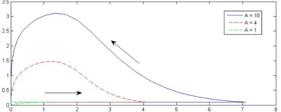
We start with considering the case when there is only one external event at time t = 0 with intensity A. Figure 2 illustrates the phase-plane for various intensities in this case. A difference with the dynamics caused by a single shock in the case whenhis decreasing (c.f. Remark 2 and the numerical simulations of [2, Figure 3]) is that here, for large values of A, the level of activity does not remain close to the maximum level Z0 which, we recall, is the zero of z7→G(z)−ωz.
Figure 2: The (v, u) phase-plane obtained by running simulations of system (1) withh(u) satisfy-ing (4) and parameters θ= 0.7, Z0= 4.4, p=−0.7 with various levels of intensityA.
We are able to reproduce similar results to those obtained for the single-site model whenh(u) is decreasing in [2]. First, we provide conditions that guarantee the eventual self-relaxation of the outburst of activity.
Proposition 4.1. If (u, v) is a solution to (1) with source term
S(t) =Aδ(t), A >0,
and r(0)G0(0)< ω, then u(t)→0 and v(t)→0 ast→ ∞.
The proof follows that of Proposition 1 in [2], however we include it here in order to point out the difference in the decay rate.
Proof. We can solve for the social tension explicitly:
v(t) =Ae−´0th(u(s))ds,
which we then substitute into the equation (1a) to obtain:
ut(t) =−ωu(t) +r
Ae−´0th(u(s))ds)
G(u(t)).
Since h is monotone increasing we have the following lower bound:
ˆ t
0
h(u(s))ds≥h(0)t, (20)
Recall that in [2] the authors studied the specific form ofh(u) given by (4) withp >0. Partic-ularly, the proof of Proposition 1 from [2] gives the lower bound:
h(u)≥ θ
(1 +Z0)p.
From the above proof we see that
v(t)≤
(
Ae−θt for p <0,
Ae−
θ
(1+Z0)pt p >0.
So that bothu(t) andv(t) are thus expected to decay faster in the casep <0. Furthermore, as in the case when p > 0 we have prolonged periods of activity with strong enough intensity of the external event. This is stated in the following proposition.
Proposition 4.2. Given arbitrary L >0 andδ >˜ 0,there exists AL,˜δ=AL,˜δ(L,δ˜) and t0>0such
that if A≥AL,δ˜ then
u(t)> Z0−δ˜ ∀ t∈[t0, t0+L].
The proof of Proposition 4.2 follows that of Proposition 2 in [2] with only minor modification; therefore, we omit it. However, we note that these changes enable us to see that for a given Land
δ > 0 a larger value of A is required for the case when h(u) is increasing than for the case when
h(u) is decreasing.
4.2 Satbility of the quiet cycle and existence of excited cycles
Let us come back to the case of a periodic source termSsatisfying (3). We prove here Theorem 1.3. On one hand we show that the tension inhibitive assumption allows one to improve the result of Proposition 2.2 in the caseA < A0, namely the quiet cycle is a global attractor. On the other hand
we use a variant of Brouwer’s fixed point theorem in order to prove the existence of an excited cycle
when A > A0.
Proof of Theorem 1.3. Case A < A0.
It follows from (9) and the monotonicity of hthat
lim sup
n→∞
v(nT)≤lim sup
n→∞
A
n
X
j=1
e−
´nT
jT h(u(s))ds ≤A ∞
X
k=0
e−kT h(0) =V .
Thus, by (1), as n→ ∞we have that
∀t∈[0, T), v(nT +t)≤V e−h(0)t+o(1),
and then that
∀t∈[0, T), (ut/u)(nT +t)≤r(V e−h(0)t)G0(0)−ω+o(1),
which entails
log(u((n+ 1)T))−log(u(nT))≤G0(0)
ˆ T
0
r(V e−h(0)t)dt−ωT +o(1).
Recalling the definition (10) of A0 we see that A < A0 implies that the right-hand side is less than
Case A > A0.
Owing to Proposition 2.2 part (ii), we only need to show that the system admits an excited cycle. This will be achieved by constructing a set Qwhich does not contain (0, V), is invariant under the mapping E (i.e. E(Q) ⊂ Q) and is homomorphic to a convex, compact set. It will then follows immediately from Brouwer’s theorem that E admits a fixed point in Q (see, e.g., [24]). The fixed point is the initial datum of a cycle which is excited because (0, V)∈/ Q. The difficulty to obtain an invariant set which does not contain the point (0, V) is that the latter is unstable just with respect to perturbation in the U component, but it is stable in the V component. This is why we need to construct a set which does not intersect the{U = 0}axis.
Note preliminarily that any solution (u, v) withu(0)≤Z0 and v(0)≤V satisfiesu ≤Z0 for all times due to (5), and by the monotonicity ofh
v(T) =v(0)e−
´T
0 h(u(s))ds+A≤V e−h(0)T +A=V .
Namely,
E([0, Z0]×[0, V])⊂[0, Z0]×[0, V]. (21)
We define a family of polygons{Pn}by settingP0:= [ρ, Z0]×[0, V], withρto be chosen, and then,
by iteration,
Pn+1 :=Pn ∪ [Un, Z0]×[Vn, V],
where
Un:= min{U : (U, V)∈ E(Pn)\Pn}, Vn:= min{V : (U, V)∈ E(Pn)\Pn}.
ClearlyE(Pn)⊂Pn+1 for all n∈N. Two situation can occur: eitherE(Pn˜)⊂Pn˜ for some ˜n, or
E(Pn)\Pn =6 ∅ for all n and thus the above procedure provides us with an infinite sequence{Pn}.
In the first case Q:=Pn˜ will be our invariant set. Consider the second case. We claim that, forρ
suitably small, there exists ˜nsuch that
V1 <· · ·< V˜n, V˜n≥V −ε0, (22)
where, throughout the proof, ε, ε0 are given by Lemma 2.1. Let (u, v) be a solution to (1). We compute
V −v(T) =V −v(0)e−
´T
0 h(u(s))ds−A= V −v(0)e−h(0)T +v(0) e−h(0)T −e−
´T
0 h(u(s))ds.
Note that the last term is close to 0 if u(0)∼0. Hence, takingρ small enough, we find a constant
k∈(e−h(0)T,1) such that the following implication holds:
(
u(0)< ρ
v(0)< V −ε0 =⇒ V −v(T)≤k(V −v(0)). (23)
Consider n ≥ 1 and (U, V) ∈ E(Pn)\Pn, that is, (U, V) = E( ˜U ,V˜) with ( ˜U ,V˜) ∈ Pn such that
E( ˜U ,V˜)∈/ Pn. Since by definition
Pn ⊃ Pn−1∪(E(Pn−1)\Pn−1) ⊃ E(Pn−1),
we have that ( ˜U ,V˜) ∈/ Pn−1 ⊃P0, then in particular, ˜U < ρ and ˜V ≥Vn−1. If ˜V ≥V −ε0 then,
therefore, taking the minimum over E(Pn)\Pn, this inequality holds true with V replaced by Vn.
This entails that{Vn} is increasing as long as it is smaller thanV −ε0, and thatVn≥V −ε0 forn
larger than or equal to some ˜n. Namely, (22) holds. Finally, the set
Q:=Pn˜∪[Un˜, Z0]×[V −ε0, V]
is invariant under E. Indeed, from one hand (22) entails
E(Pn˜) ⊂ Pn˜+1 = Pn˜∪[Un˜, Z0]×[Vn˜, V] ⊂ Q,
and from the other if (U, V) ∈ [U˜n, Z0]×[V −ε0, V] then either U ≥ ρ, in which case E(U, V) ∈
P1⊂Q, orU < ρand thus Lemma 2.1 yields E(U, V)∈[Un˜, Z0]×[V −ε0, V].
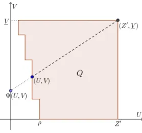
Figure 3: The invariant set for E.
We have therefore constructed an invariant set Qof the following type
Q=
˜ n
[
n=0
[Un, Z0]×[Vn, V],
with min0≤n≤n˜Un >0 and min0≤n≤˜nVn = 0 (see Figure 3). It is clear that a set of this this type
is homomorphic to the rectangle [0, Z0]×[0, V] (for instance through the function Ψ which, for any (U, V) in the closure of (∂Q)∩(0, Z0)×(0, V), “stretches” the segment from (Z0, V) to (U, V) up to reaching one of the coordinate axis, in an affine way). Alternatively one can easily construct a retraction of [0, Z0]×[0, V] into Q (that is, a continuous function coinciding with the identity on
Q) and then apply [24, Theorem 2.1.5] to obtain a fixed point. This concludes the proof.
Remark 3. An easier argument allows one to prove a weaker form of Theorem 1.3. Namely, that
when A > A0 the system admits an excited n-cycle (i.e. a solution with period nT) for n large
enough. The argument reduces to finding a closed rectangle which does not intersect the {u= 0}
axis and is invariant under some power ofE. This is achieved exploiting property (11). Recall that the quantity n0, η appearing there depend on the solution (u, v) only through an upper bound ofu
and v. Hence, because of (21), property (11) holds with the samen0, η for all solutions with initial datum in [0, Z]×[0, V]. Thus, any solution (u, v) with initial datum in [0,min{η, Z}]×[0, V] satisfies
|v(n0T)−V|< ε0. Then, applying recursively Lemma 2.1 we derive the following implication:
and the latter inequality implies, by (6), u((n0+n)T) ≥ (1 +σ)ne−ωn0Tu(0). Therefore, taking
n00∈Nsuch that (1 +σ)n 00
e−ωn0T ≥1, we deduce thatu((n0+n00)T)≥u(0) provided the hypothesis in (24) holds for n = n00. Instead, if it does not, there exists m ∈ {0, . . . , n00 −1} for which
u((n0+m)T)> ε, whence
u((n0+n00)T)≥e−ω(n00−m)Tu((n0+m)T)> εe−ωn00T.
This shows that, in any case, if u(0) ∈ [ρ, η] with ρ ≤ εe−ωn00T, then u((n0 +n00)T) ≥ ρ. Let us consider the case (u(0), v(0)) ∈ (η, Z]×[0, V]. Always by Gr¨onwall’s inequality, there holds
u((n0+n00)T)> ηe−ω(n0+n00)T. Combining this estimate with the previous one we eventually deduce
that the rectangle
[ρ, Z]×[0, V] with ρ= min{εe−ωn00T, ηe−ω(n0+n00)T}
is invariant under the operatorEn0+n00. The fixed point provided by Brouwer’s theorem is the initial
datum of an excited (n0+n00)-cycle.
Note that if there were not a cycle then the above property would provide infinite manyn-cycles: the ones with nprime larger than n0+n00. This would have been hard to believe.
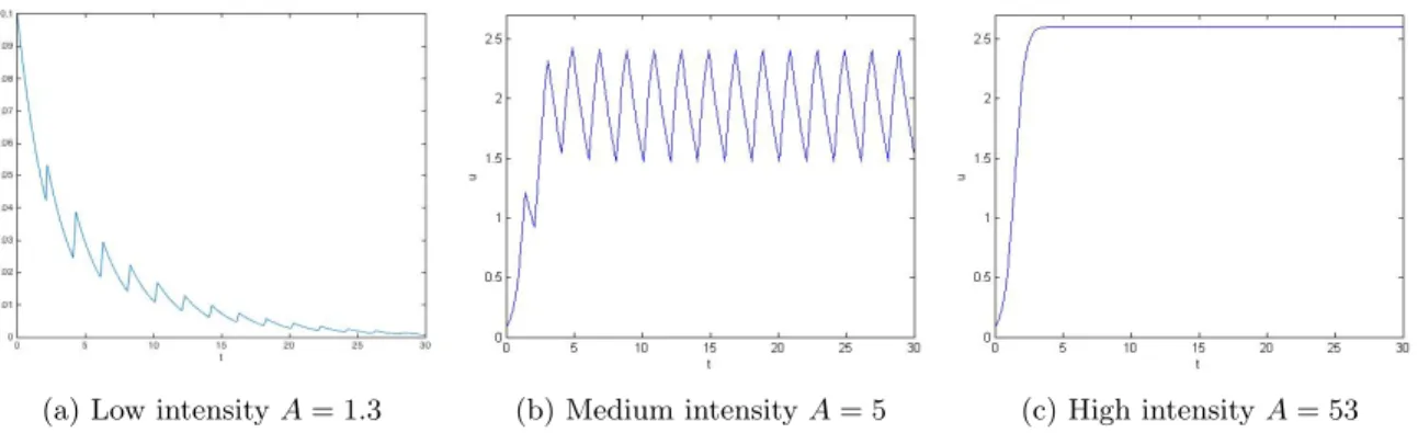
4.3 Asymptotic convergence to cycles when r is the step function
This section is dedicated to the proof of Theorem 1.4. Namely, we consider here the case where r
is the step function1[a,∞), leading to a dichotomy in the system: ifv(t)< athenu(t) is decreasing
exponentially to zero and if v(t)> a thenu(t) is increasing to Z0. In the former case we say that the system is in the relaxed stateand in the latter we say that the system is in the excited state. If it definitely remains in one of such states, the system is basically decoupled. This allows us to prove the convergence to the excited cycle with maximal u component when A is above a threshold ¯A. Conversely, we show that this convergence does not occur below such threshold.
Proof of Theorem 1.4. Consider the solution (u, v) with initial datum (U, V)∈R2
+. There holds
lim sup
t→∞
u(t)≤Z0. (25)
This property follows immediately from the fact that suput < 0 in the regions where infu > Z0,
regardless of whether the system is in the relaxed state v < aor in the excited statev≥a.
Let us start with proving the second statement of the theorem. Suppose firstly thatU ∈(0, Z0],
which implies that u∈(0, Z0] for all times. Now, given that h(u) is increasing we obtain from the explicit expression of v (9) that
∀t∈[(n−1)T, nT), n∈N, v(t)≥V e−h(Z0)t+A
n−1
X
j=1
e−(t−jT)h(Z0).
Let us consider what happens to the sequence{v(nT−)}asn→ ∞, wherev(nT−) = limt→nT−v(t).
We have the following lower bound:
v(nT−)≥V e−h(Z0)nT +A
n−1
X
j=1
e(n−j)h(Z0)T =V e−h(Z0)nT +A
n−1
X
k=1
e−kh(Z0)T.
and therefore
lim inf
n→∞ v(nT
−)≥A ∞
X
k=1
e−kh(Z0)T = A
eh(Z0)T
The hypothesisA >A¯ of the theorem is precisely what ensures the latter term to be larger thana, whence v(nT−) > a for n large enough. Finally, since v(t) > v(nT−) for t ∈ [(n−1)T, nT), we eventually deduce that v(t) > a for sufficiently large t in the case A > A¯. Thus, if A > A¯,
ut(t) = G(u(t)) for large t, which readily implies thatu(t)→ Z0 ast→ ∞. Notice that the same
holds true if U > Z0. Indeed, in such case, eitheru(t∗) =Z0 at some timet∗ and then u(t)≤Z0 for all t≥t∗ and we end up with the previous case, or u > Z0 for all times and the conclusion follows from (25). It remains to show that v is asymptotically periodic. Again by (9) we compute
lim
n→∞v(nT) =Anlim→∞
n
X
j=1
e−(n−j)T
fflnT
jT h(u(s))ds =A lim
n→∞
n−1
X
k=0
e−kT
fflnT
(n−k)Th(u(s))ds.
Using the fact that u(∞) =Z0 it is straightforward to check that ffl(nTn−k)T h(u(s))ds→ h(Z0)ds as
n → ∞, uniformly with respect to k ∈ {0, . . . , n−1}. Thus, limn→∞v(nT) is controlled by the
geometric series AP∞
k=0e
−k(h(Z0)±ε)T for arbitraryε >0, whence
lim
n→∞v(nT) =A ∞
X
k=0
e−kh(Z0)T = A
1−e−h(Z0)T =:V .
This shows that, fort∈[0, T),v(nT+t)→V e−h(Z0)tasn→ ∞, concluding the proof of the second statement of the theorem.
Next, we prove the first statement. The idea is that ifu → Z0 along some sequence, then it is close toZ0in arbitrarily large intervals and thusvis necessarily larger thanain such intervals. This is impossible if A <A¯. So, assume by contradiction that the inequality in (25) is not strict. Let us suppose for the moment that U ≤Z0. Consider a diverging sequence {tn} such thatu(tn)→Z0
as n → ∞. By the Arzel`a–Ascoli theorem, the sequence of functions u(·+tn) converges (up to
subsequences) locally uniformly inRto a function ˜u satisfying ˜u≤Z0 inRand ˜u(0) =Z0, together
with the integral inequality
∀t <0, Z0−u˜(t)≤
ˆ 0
t
G(˜u(s))−ωu˜(s)ds.
The function w defined byw(t) :=Z0−u˜(−t) satisfiesw(0) = 0 and
∀t >0, w(t)≤
ˆ 0
−t
G(˜u(s))−ωu˜(s)ds=
ˆ t
0
G(˜u(−s))−ωu˜(−s)ds=
ˆ t
0
β(−s)w(s)ds,
where β is defined by
β(t) :=
−G(˜u(t))−ωu˜(t)
˜
u(t)−Z0 if ˜u(t)6=Z
0
−G0(Z0) +ω if ˜u(t) =Z0.
Notice thatβ is positive and continuous because z7→G(z)−ωz is positive in (0, Z0) and vanishes at Z0. It follows from the integral Gr¨onwall inequality that w(t) ≤ 0 fort ≥0, that is, ˜u(t) =Z0
fort≤0. This means thatu(·+tn)→Z0 asn→ ∞ locally uniformly on (−∞,0]. If we now drop
the assumption U ≤ Z0 we have that either u becomes eventually smaller than Z0 – and then the previous case applies – or u > Z0 for all times and then u(∞) = Z0. Therefore, the convergence to Z0 on the left of a sequence {tn} holds in any case. We now use this information to derive the
asymptotic behavior ofv. Specifically, consider a sequence{kn}inNsuch thattn∈[knT,(kn+1)T).
Then, for any m∈ {1, . . . , kn}, applying (9) tov(·+ (kn−m)T) we deduce
v(knT−) =v((kn−m)T)e− ´mT
0 h(u(s+(kn−m)T))ds+A
m−1
X
j=1
e−
´mT