Groupwise Shape Correspondence with Local
Features
˙Ipek O˘guz
A dissertation submitted to the faculty of the University of North Carolina at Chapel Hill in partial fulfillment of the requirements for the degree of Doctor of Philosophy in the Department of Computer Science.
Chapel Hill 2009
Approved by:
Martin A. Styner, Advisor
Marc Niethammer, Co-principal Reader
Stephen M. Pizer, Reader
J. Stephen Marron, Reader
c 2009 ˙Ipek O˘guz
Abstract
˙Ipek O˘guz: Groupwise Shape Correspondence with Local Features. (Under the direction of Martin A. Styner)
Statistical shape analysis of anatomical structures plays an important role in many medical image analysis applications such as understanding the structural changes in anatomy in various stages of growth or disease. Establishing accurate correspondence across object populations is essential for such statistical shape analysis studies. How-ever, anatomical correspondence is rarely a direct result of spatial proximity of sample points but rather depends on many other features such as local curvature, position with respect to blood vessels, or connectivity to other parts of the anatomy.
This dissertation presents a novel method for computing point-based correspon-dence among populations of surfaces by combining spatial location of the sample points with non-spatial local features. A framework for optimizing correspondence using arbitrary local features is developed. The performance of the correspondence algorithm is objectively assessed using a set of evaluation metrics.
Acknowledgments
I’d like to express my gratitude to those who have contributed to this work. First, I would like to thank Martin Styner for being an outstanding advisor and mentor during these 5 years. It makes me happy to know that our collaboration is not coming to an end. I am also very grateful to my committee members. In particular, Marc Niethammer has been extremely helpful with the preparation of this document with his detailed (and extremely fast!) feedback as well as his insights throughout the project. It has been a privilege to learn from Steve Pizer, whose immense knowledge and understanding of the field as well as his enthusiasm for his work is a constant source of inspiration. I am thankful to Steve Marron for lending his statistical expertise and to Ross Whitaker for a very productive collaboration throughout the project.
I’d like to thank Josh Cates who generously shared his knowledge, insights, code and time throughout this project. Tom Fletcher has been a great mentor and friend who gave me advice on what classes to take during my first semester, what to expect at job interviews during my last semester, and everything in between (including bird watching advice that I completely ignored, sorry). The MDL-based portion of this work wouldn’t have been possible without the very patient and friendly Tobias Heimann. The MIDAG team at UNC has been a constant source of knowledge, ideas and support.
I am thankful to Randy Gollub and the MIND Clinical Imaging Consortium for the main cortical dataset, and to Stephen Aylward and Derek Cool for the remaining cortical data. The caudate and striatum segmentations were provided by James Levitt and Martha Shenton, the femur segmentations were provided by Markus Fleute, and the lateral ventricle segmentations were provided by Daniel Weinberger and Douglas Jones.
This work was supported by the National Alliance for Medical Image Computing (NA-MIC), funded by the NIH. I have been incredibly fortunate to be part of NA-MIC; I am absolutely grateful for the opportunity to meet and collaborate with many great researchers.
Table of Contents
List of Figures . . . x
List of Abbreviations . . . xii
1 Introduction . . . 1
1.1 Correspondence of local features . . . 2
1.2 Framework for correspondence of local features without parametrical mapping . . . 3
1.2.1 Application to the human brain: dealing with the geometric challenges of the cortex . . . 5
1.3 Using white matter fiber structure for cortical correspondence . . . . 6
1.3.1 Probabilistic connectivity . . . 7
1.3.2 Mapping the connectivity to the cortical surface . . . 7
1.4 Evaluation of correspondence quality . . . 9
1.5 Thesis and contributions . . . 10
1.6 Overview of chapters . . . 11
2 Shape Correspondence . . . 13
2.1 Pairwise Correspondence . . . 14
2.1.1 Surface-based pairwise correspondence . . . 14
2.1.2 Volume-based pairwise correspondence . . . 21
2.2 Groupwise Correspondence . . . 23
2.2.2 Minimum Description Length . . . 24
2.3 Correspondence Evaluation . . . 25
2.3.1 Distance to Manual Landmarks . . . 25
2.3.2 Jaccard Coefficient Difference . . . 26
2.3.3 Generalization, Specificity and Compactness . . . 27
2.3.4 Goodness of Predictionρ2 . . . 29
3 Parameterization-Based Group Correspondence . . . 30
3.1 Traditional MDL . . . 30
3.1.1 Original Algorithm Formulation . . . 31
3.1.2 Gradient Descent Optimization of the MDL Function . . . 33
3.1.3 Shape Image Based MDL Optimization Schemes . . . 35
3.2 Generalized MDL Correspondence . . . 35
3.2.1 Using Local Features for Generalizing MDL . . . 36
3.3 Geometric Features . . . 37
3.3.1 Principal Curvatures (κ1, κ2) . . . 37
3.3.2 Mean Curvature and Gaussian Curvature (H, K) . . . 38
3.3.3 Curvedness and Shape Index (C, S) . . . 38
3.4 Results and Discussion . . . 40
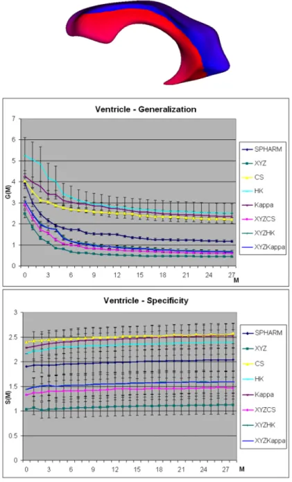
3.4.1 Lateral Ventricle . . . 43
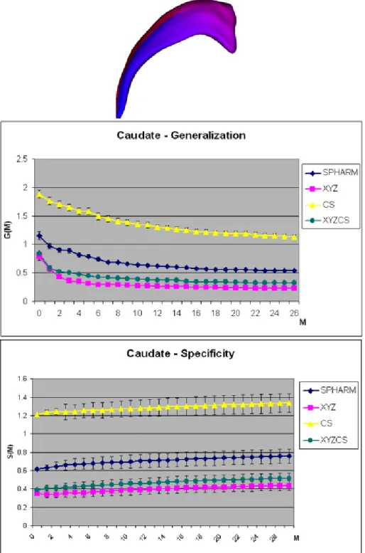
3.4.2 Caudate . . . 44
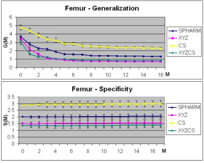
3.4.3 Femur . . . 44
3.4.4 Striatum . . . 44
3.4.5 Discussion . . . 45
4.1 Entropy-based Particle Framework . . . 52
4.1.1 Surface entropy . . . 52
4.1.2 Ensemble entropy . . . 55
4.2 Generalized ensemble entropy . . . 57
4.3 Application to cortex . . . 58
4.4 Surface interpolation from particles . . . 60
4.5 Results . . . 63
5 DTI-based Connectivity for Cortical Correspondence . . . 69
5.1 Diffusion Tractography for Connectivity . . . 71
5.1.1 Streamline tractography . . . 71
5.1.2 Stochastic tractography . . . 72
5.1.3 Optimal path methods . . . 74
5.2 Mapping Connectivity to the Cortical Surface . . . 75
5.2.1 Kernel-based averaging . . . 75
5.2.2 Brain deflation . . . 76
5.3 Results . . . 82
6 Discussion . . . 87
6.1 Summary of contributions and thesis . . . 87
6.2 Future work and discussion . . . 94
Appendix A: Spherical Harmonics . . . 99
A-1 Surface representation . . . 99
A-2 Partial derivatives . . . 100
A-3 Surface normal . . . 103
A-4 First and second fundamental forms . . . 103
List of Figures
1.1 Pipeline overview . . . 8
2.1 Example of parameterization-based correspondence . . . 16
3.1 Issues with using spatial proximity as a correspondence indicator . . . 36
3.2 Shape indexS . . . 39
3.3 Curvedness C . . . 40
3.4 The relative locations of the various brain structures used in experiments 41
3.5 The results of the SPHARM, traditional MDL and CombinationMDL demonstrated on two striata and two femoral heads . . . 42
3.6 Comparison of correspondence results for lateral ventricle population 47
3.7 Comparison of correspondence results for caudate population . . . 48
3.8 Comparison of correspondence results for femur population . . . 49
3.9 Comparison of correspondence results for striatum population . . . . 50
4.1 Sulcal depth on the white matter (WM) surface and the inflated WM surface . . . 60
4.2 Surface interpolation from particles . . . 61
4.3 Example of surface interpolation . . . 62
4.4 Correspondence results comparison for the first cortical dataset . . . 64
4.5 Comparison of the distribution of variance across the cortical surfaces for entropy method and FreeSurfer . . . 65
4.6 Correspondence results comparison for the second cortical dataset . . 66
4.7 Cortical thickness generalization,G(M) . . . 67
5.1 Connectivity features pipeline overview . . . 70
5.2 Impact of brain deflation algorithm on surface connectivity values . . 76
5.3 Brain deflation progress for one subject . . . 79
5.4 Motivation for normalizing connectivity maps . . . 80
5.5 Comparison of connectivity maps with linear normalization and his-togram equalization . . . 81
5.6 Correspondence results comparison using average variances of cortical thickness and sulcal depth . . . 84
List of Abbreviations
MRI Magnetic Resonance Imaging, introduced chapter 1
MRA Magnetic Resonance Angiography, introduced chapter 1
MDL Minimum Description Length, introduced section 1.1
WM White Matter, introduced section 1.2
GM Gray Matter, introduced section 1.2
DTI Diffusion Tensor Imaging, introduced section 1.3
DWI Diffusion Weighted Imaging, introduced section 1.3
ROI Region of Interest, introduced section 1.3
SPHARM Spherical Harmonics, introduced section 2.1.1
SPM Statistical Parametric Mapping, introduced section 2.1.2
FMRIB Oxford Center for Functional MRI of the Brain, introduced section 2.1.2
FSL FMRIB Software Library, introduced section 2.1.2
PCA Principal Components Analysis, introduced section 2.2
ASM Active Shape Models, introduced section 2.2
Chapter 1
Introduction
The variability of anatomical structures among individuals is large within anatomical populations. This variability makes it necessary to use statistical modeling tech-niques to study shape similarities and to assess deviations from the healthy range of variability. For instance, studying the local cortical thickness measurements of the brain is a common tool for studying many medical conditions such as autism and Alzheimer’s disease in humans. Statistical analysis of anatomical objects is there-fore becoming increasingly important in segmentation, analysis and interpretation of medical datasets.
The construction of such statistical models requires the ability to compute local shape differences among similar objects, which introduces the problem of finding cor-responding points across the population. Consistent computation of corcor-responding points on 3D anatomical surfaces is a difficult task, since manually choosing landmark points not only is cumbersome, but also does not yield a satisfyingly dense correspon-dence map. It should also be noted that no generic “ground truth” definition of dense correspondence exists across different anatomical surfaces. The choice of particular correspondence metric must, therefore, be application-driven.
emphasis is given to the human cortical surface using Magnetic Resonance Imaging (MRI) scans. The correspondence computation on the cortex is a highly challenging problem due to the convoluted geometry of the brain and the high variability of fold-ing patterns across subjects. Usfold-ing mere spatial locations of surface points produces a weak and inadequate correspondence map. My work allows the use of additional local information, called ‘features’ throughout this manuscript, for computing cor-respondence. These features can be structural, such as sulcal depth measurements, as well as nonstructural, such as connectivity maps computed from Diffusion Tensor Imaging (DTI) images, or vessel structure extracted from Magnetic Resonance An-giography (MRA) images. The particular choice of features should be determined by the target applications. This dissertation in particular explores various features that can be extracted from DTI scans.
1.1
Correspondence of local features
Previous population-based correspondence computation methods, such as Minimum Description Length (MDL) [1, 2], optimize correspondence by minimizing the covari-ance of the sample locations across the population. These methods work well for objects of simple enough geometry, such as caudates, but are inadequate with objects of complex geometry with rapidly changing curvature values across the surface, such as femoral heads or striata.
replacing the data matrix in MDL, which contains the spatial location of each sample point of each object in the population, by a matrix that contains the desired local feature value at each sample point of each object.
Using this framework, I show that using a version of MDL based on solely curva-ture values leads to poor correspondence, since the curvacurva-ture values are not unique across the object surfaces. However, using a combination of spatial position and local curvature improves the correspondence quality significantly for objects of complex geometry, and it gives similar results to traditional (location-only) MDL for objects of simple geometry. In this context, correspondence quality is measured by using the generalization and specificity properties of the statistical model of the population that results from the correspondence optimization, as discussed later in detail.
These results show that there is room for improvement of the correspondence quality by exploring local features other than spatial location. My framework allows for the use of any local feature whose absolute difference defines a metric in the feature space, as long as the feature values at each sample point are provided as input to the system.
The choice of the particular feature set to be used should be made based on the application context; one of the novel contributions of this dissertation is the exploration of possible features to be used for optimizing the correspondence of the human cortex. The ideal feature set would provide enough variability across the object surface and across the population.
1.2
Framework for correspondence of local features
without parametrical mapping
limited applicability to human cortex. The available implementations of the algo-rithm rely on a spherical parameterization of the surfaces, which is computationally expensive to obtain for the cortical surface (defined as the white matter (WM) - gray matter (GM) boundary) given the complex geometry. It also is computationally very expensive for high resolution meshes that are necessary for representing the cortical surface. Therefore, the current formulation of MDL is not suitable for the cortical correspondence optimization. However, it is a well-known fact in information theory that MDL is, in general, equivalent to minimum entropy (min log|Σ +αI|, where Σ is the covariance matrix of the population and αI is a diagonal regularization ma-trix that introduces a lower bound α to the eigenvalues of the covariance matrix). Therefore, I chose to use an entropy-based dynamic particle framework introduced by Cates et al.[3, 4] as my starting point. The entropy-based correspondence scheme does not require a spherical topology and is much more computationally efficient. I propose a solution to the problems caused by the geometric complexity of the cortex in Section 1.2.1.
The main idea for the entropy-based correspondence method is to construct a point-based sampling of the shape ensemble that simultaneously maximizes a combi-nation of the geometric accuracy and the statistical simplicity of the model. Surface point samples, which also define the shape-to-shape correspondences, are modeled as sets of dynamic particles that are constrained to lie on a set of implicit surfaces. Sample positions are optimized by gradient descent on an energy function that bal-ances the negative entropy of the points’ distribution on each shape, which represents an even sampling of the individual surfaces, with the positive entropy of the ensem-ble of shapes, which represents a high similarity of corresponding points across the population.
feature values in the ensemble entropy term, in lieu of the spatial locations. The surface entropy term remains the same, since this term ensures an even sampling of the surfaces regardless of the local feature values. The incorporation of the local features in the particle framework requires a modification to the ensemble entropy term. Consequently, the associated gradient has to change, which can be accomplished via the chain rule.
1.2.1
Application to the human brain: dealing with the
geo-metric challenges of the cortex
One of the main constraints of the entropy-based correspondence method is that it assumes the particles exist on local tangent planes of the surface. This assumption makes it possible to avoid the costly computation of geodesic distances on the surface. However, the assumption becomes problematic for surfaces of a highly convoluted geometry, such as the human cortex. I overcome this problem by first ‘inflating’ the cortex to obtain a less convoluted surface. The particles live and interact on this blob-like surface; however, the local feature values, such as curvature and sulcal depth, are still associated with the original surface. A one-to-one correspondence between the original cortex surface and the inflated surface is therefore needed.
A set of automated tools, distributed as part of the FreeSurfer package [5, 6, 7, 8, 9, 10], are used to inflate the cortical surface, as well as to perform surface reconstruction. However, any other surface reconstruction and inflation pipeline could easily be used to replace FreeSurfer, since my algorithm does not depend on the specific FreeSurfer methodology.
inflation. It should be noted that sulcal depth captures the high level foldings of the cortical surface but is relatively insensitive to the smaller folds; this property makes sulcal depth an attractive correspondence metric since it is relatively stable across individuals, in addition to being available across the whole cortical surface.
1.3
Using white matter fiber structure for cortical
correspondence
The choice of suitable local features is central to the quality of correspondence results. For the cortical correspondence problem, I propose to use a feature set derived from Diffusion Tensor Imaging (DTI) scans of the subjects in order to incorporate available knowledge about the white matter (WM) fiber tracts of the brain in addition to the structural features discussed earlier. Structural MRI scans show white matter homo-geneously, such that it is impossible to infer the orientation of the fiber tracts within each voxel. The understanding of the white matter structure, however, can be largely improved by additional information on fiber tracts that can be fully automatically extracted from DTI data.
The main challenge is to find a suitable mapping of the fiber tract structure to the cortical surface. Probabilistic connectivity maps, which represent for each voxel on the cortical surface the probability of its being connected via fiber tracts to a given region of interest (ROI), is the proposed solution to this problem.
1.3.1
Probabilistic connectivity
The probabilistic connectivity maps are obtained via stochastic tractography. For every voxel in the white matter, the connectivity probability to various ROI’s is computed via a Monte Carlo approach. In this dissertation, I use a stochastic trac-tography implementation, described by Ngo [11], based on a modification of Friman’s algorithm [12, 13]. In this approach, fiber tracts are modeled as sequences of unit vectors whose orientation is determined by sampling a posterior probability distri-bution. The posterior distribution is proportional to a prior of the fiber orientation multiplied by the likelihood of the orientation given the Diffusion Weighted Imag-ing (DWI) data. The trackImag-ing stops when the tract either reaches a voxel with a low probability of belonging to the white matter, or it exceeds a predetermined maximum length, or it makes an improbably sharp turn. In order to estimate the probabilistic connectivity with appropriate accuracy, a high number of sample fibers need to be tracked from each voxel included in the input ROI. The probabilistic connectivity of a voxel to the ROI is then defined as the ratio of fiber samples that travel through a voxel to the total number of samples.
The connectivity to each separate ROI is represented as a separate feature in the particle framework. It should be noted that the spatial features used in the correspondence (such as the sulcal depth) have to be normalized to match the range of values of the connectivity probabilities, in order to avoid assigning a heavier weight to the spatial features.
1.3.2
Mapping the connectivity to the cortical surface
Figure 1.1: Pipeline overview. I use T1 images to generate white matter (WM) sur-faces and inflated cortical sursur-faces, as well as local sulcal depth. Selected ROI’s and the DWI image are input to the stochastic tractography (ST) algorithm. WM sur-face deflated using proposed algorithm is used to construct connectivity maps on the surface from ST results. Inflated cortical surfaces and the connectivity maps are used to optimize correspondence. Note that there are three different surfaces representing the cortex. The original surface is used for the computation of the geometrical fea-tures, such as sulcal depth. The inflated surface is used for the computation of the particle inter-distances. The deflated surface is used for evaluating the connectivity probabilities.
after the stochastic tractography algorithm is executed. The connectivity probability values assigned by the stochastic tractography algorithm strongly correlate with sulcal depth. Directly using these probabilities for correspondence optimization is therefore not appropriate.
1.4
Evaluation of correspondence quality
In order to evaluate the proposed framework, I apply my proposed techniques to a small set of clinical studies and compare the results with other existing algorithms. This is for evaluation purposes only, in order to compare the performance of my algorithm with others. Thorough validation studies are outside the scope of this dissertation.
Metrics for assessing correspondence quality are necessary to compare the dif-ferent correspondence algorithms. For this purpose, I analyze the generalization and specificity properties of the resulting shape models. Lower variability as well as better generalization and specificity properties point to an improved correspondence across the population. I use the cortical thickness measurements to compute the generaliza-tion and specificity for the cortical datasets, instead of the surface sample locageneraliza-tions. Location-based analysis is considered biased since both my technique and many other algorithms use the surface sample locations for the optimization; the cortical thick-ness provides an unbiased measurement more suitable for evaluation. I also present visual assessments of correspondence quality where suitable.
1.5
Thesis and contributions
Thesis: Statistical shape analysis of anatomical structures, which is essential to un-derstanding the structural changes in anatomy in various stages of growth or
dis-ease, requires establishing accurate correspondence across object populations.
How-ever, anatomical correspondence is rarely a direct result of spatial proximity of
sam-ple points on the surface. A generalized correspondence framework that incorporates
the similarity of non-spatial local features provides a more accurate correspondence
of sample points across populations of surfaces. In particular, incorporating features
based on cortical geometry as well as the fiber connectivity of the white matter
signif-icantly improves correspondence of the human cortical surfaces.
The contributions of this dissertation are as follows:
1. I demonstrate that the use of an approach allowing for the incorporation of arbitrary local features into the similarity metric to be used for correspondence optimization enhances correspondence, as measured by objective evaluation cri-teria.
2. I present a novel parametric groupwise correspondence optimization method that allows using arbitrary local features for establishing correspondence.
3. I demonstrate that using geometric information, such as local curvature mea-sures, as additional local features improves correspondence quality when the objects in the population exhibit complex geometry.
4. I present a novel nonparametric groupwise correspondence optimization method that allows using arbitrary local features for establishing correspondence.
problem by producing surfaces smooth enough to avoid these challenges. Fur-thermore, I show that cortical correspondence significantly improves when sulcal depth is used as an additional local feature.
6. I present a novel framework for integrating white matter fiber connectivity in-formation into cortical correspondence, the first such method that uses fiber connectivity patterns to establish structural correspondence. To this end, I compute probabilistic connectivity maps from diffusion weighted images via a stochastic tractography algorithm. I project these connectivity values to the cor-tical surface by a new corcor-tical deflation algorithm. I present empirical evidence showing that using connectivity features enhances cortical correspondence.
7. I develop open-source software that implements all the above techniques, as well as a visualization tool that allows qualitative examination of the surfaces, the local features associated with them and the surface samples used in the correspondence algorithm.
1.6
Overview of chapters
The remainder of this dissertation is organized as follows.
Chapter 2 contains an overview of concepts and existing methodology regard-ing the correspondence problem as well as techniques for evaluatregard-ing correspondence quality.
Chapter 3 describes a novel methodology for integrating local features into the optimization of parameter-based shape correspondence and demonstrates, using ap-plications to a variety of clinical datasets that using local features can strongly im-prove correspondence. The suggested methodology is an extension to the traditional Minimum Description Length algorithm.
and without local features. This methodology is no longer dependent on a particular parameterization of the surface. This chapter also discusses some issues regarding the application of this technique to the human cortical surface, and it presents results that demonstrate that the use of even simple geometric local features (such as sulcal depth) is beneficial to correspondence quality.
Chapter 5 discusses the proposed methodology for integrating DTI-based connec-tivity information into cortical correspondence. This technique computes connecconnec-tivity probabilities via stochastic tractography and applies a surface evolution algorithm to deflate the cortical surface in order to map the connectivity probabilities to the cor-tical surface. It presents experimental results that show, via an evaluation based on cortical thickness, that the additional knowledge of white matter structure signifi-cantly improves correspondence quality.
Chapter 2
Shape Correspondence
2.1
Pairwise Correspondence
Pairwise correspondence methods aim to optimize the correspondence between each object in a given population and either a labeled atlas or one of the objects in the population chosen to serve as a template. Correspondence optimization can be done based on either surface representations or volumes. Surface-based correspondence methods typically lend more weight to geometrical properties of the objects, whereas volume-based methods focus on image intensities. Further classification can be done based on whether the algorithm aims for an exact match or an approximate match enforced by a soft penalty.
2.1.1
Surface-based pairwise correspondence
In most surface-based schemes, correspondence is defined through a parameterization of both objects, such that points in each object with the same parameter space coordinates correspond (see Fig. 2.1). Therefore, it is necessary to compute a one-to-one mapping between each object and a standard parameter space.
During the optimization stage, there are two possible ways of manipulating the correspondence: either the vertices on the surface can be moved around while keeping the parameterization fixed, or the parameterizations can be manipulated while keep-ing the surface vertices fixed. However, manipulatkeep-ing the surface vertices directly is a difficult task, since it would then be necessary not only to confine the vertices to the surface as they move in R3 but also to construct a mapping of the surface onto
itself at each iteration, a task far from trivial for arbitrary 3D surfaces. Most algo-rithms therefore choose to manipulate the parameterizations rather than the surfaces themselves.
local features for improving correspondence; however, the existing techniques focus on a preselected feature or set of features, whereas I propose a generalized framework where the user can determine what features are relevant for the particular application context.
Spherical harmonics
The spherical harmonics (SPHARM) description, introduced in [14], is commonly used as a parameterization-based correspondence scheme. Here, a continuous one-to-one mapping from each surface to the unit sphere is computed. The parameterization is defined such that it is area preserving and distortion minimizing, using a constrained optimization method. Each object is then described as a weighted sum of spherical harmonics basis functions (see Appendix A for details). The correspondence is estab-lished by rotating the parameter mesh such that the axes of their first-order spherical harmonics, which are ellipsoidal, coincide with the coordinate axes in the parameter space. Since each object can thus be parameterized without any knowledge of the others in the dataset, data sets that have significant shape variability become prob-lematic, because the SPHARM method does not have a proper means of optimizing shape similarity but rather focuses on area preservation and minimized distortion during the parameterization.
Another major shortcoming of the SPHARM correspondence is the poor handling of objects that are rotationally symmetric around the major axes with respect to the first-order ellipsoid. This often happens if the second and third axis have similar sizes. Brechb¨uhler argues that using information from higher-order harmonics can disambiguate such cases.
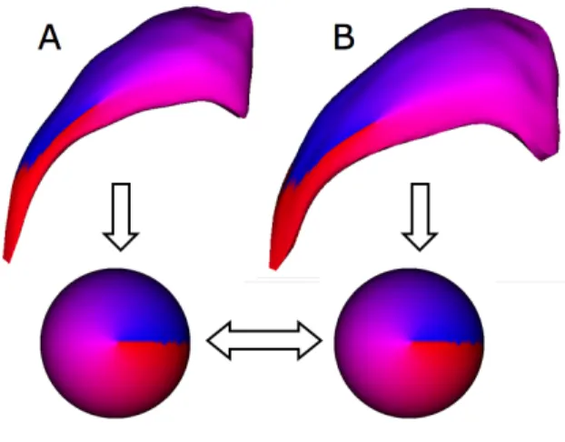
possi-Figure 2.1: Example of parameterization-based correspondence. A parameterization is computed for objects A and B individually. The correspondence is defined via the parameter space, such that points with the same parameterization correspond together when the correspond optimization is completed. Color map shows the φ
parameter, the longitude in the spherical representation.
ble flips of the parameterization and selecting the one whose reconstruction has the minimum distance to the flip template. The use of the flip template puts SPHARM correspondence in the pairwise category. An additional limitation of this method is that parameterization-based correspondence schemes in general are restricted to objects of a given topology (e.g. spherical in the case of SPHARM).
Shape-based nonrigid correspondence
Geometry driven multispectral optical flow
Tosun et al. [17] propose to use geometrical measures to align an atlas and a subject surface in a more sophisticated framework in 3D. They propose to use two curvature-related measures introduced by Koenderink [18] as the similarity metric for the cor-respondence. These measures, the shape index S and the curvedness C, decouple the shape and the size of curved surfaces and will be further discussed in Section 3.3.3. Tosun computes these curvature measures on a partially inflated cortical sur-face in order to capture only the geometry of the most prominent anatomical features to allow meaningful comparison among different individuals. This partially inflated cortical surface is obtained by a mean curvature based evolution algorithm with a preselected curvature threshold as the stopping condition. Once the shape measure maps are computed for the subject and the atlas brain, a multispectral optical flow algorithm is used to warp the subject cortical surface into the atlas using spherical parameterizations of the surfaces.
Tosun uses a surface-based iterated closest point (ICP) matching scheme [19] as an initialization point to her correspondence algorithm. This ensures that key anatomical landmarks such as major sulci are mapped to reasonably close locations on the parameter space and therefore provides a good initialization. The variational problem to estimate the optical flow field is solved using a Euclidean framework, and a gradient-descent optimization is applied.
Parameter space warping
Meier et al. [20] propose a method that represents a pair of objects using SPHARM description. However, unlike the original SPHARM correspondence, they warp the parameter space to optimize the correspondence between the two objects instead of relying on the first-order ellipsoid alignment. The objective function is a similarity metric based on Euclidean distances, normal directions and Koenderink’s shape index
S[18]. The SPHARM representation allows both a hierarchical optimization approach and the robust computation of differential features since no additional discretization error is introduced.
As with other spherical parameterization-based techniques, the method is limited to objects of spherical topology. Additionally, both the initial SPHARM computation as well as the warping procedure itself are computationally expensive and limit the practical applicability of the algorithm. For the cortical surface dataset reported in the manuscript, 24 harmonics were used, with 9126 vertices on the whole surface. While this may be an adequate representation of the surface for 5mm-thick MRI slices used in the study, it is far from satisfactory for higher resolution data commonly available nowadays.
FreeSurfer
FreeSurfer [5, 6, 7, 8, 9, 10] is an image analysis suite for brain studies. Aside from cortical reconstruction and inflation tools, FreeSurfer also offers a spherical surface-based coordinate system surface-based on a cortical correspondence optimization method. This method, described in detail in [7], is based on nonrigidly aligning each individ-ual’s folding patterns with an atlas. The folding pattern in this context is quantified by the sulcal depth of the surfaces.
parameter-izations for the individual and the atlas are morphed into register by a combination of sulcal depth alignment and isometry-preserving forces. The sulcal depth alignment is achieved by minimizing the mean squared difference between the average sulcal depth computed from a fixed training set and that of the individual modulated by the variance across the training set.
Fischl further argues that simply maximizing the sulcal depth alignment is not enough to prevent folds and distortions. He therefore introduces two additional energy terms to the objective function of the optimization. The first term is for the preser-vation of local distances, which gives the surface some local stiffness and discourages excessive shear. The second term is for area preservation and aims to prevent ex-cessive compression or expansion. These terms are weighted against the sulcal depth alignment term by free parameters.
Like the geometrically driven optical flow method described above, the FreeSurfer correspondence method ignores the spatial location of the vertices in its similarity metric definition and therefore has to resort to a nontrivial initialization procedure as well as the additional regularization terms described above. Additionally, it can produce suboptimal correspondence results since it doesn’t capture the variability of the whole population.
BrainVoyager
atlas or a designated template object in the population; however, BrainVoyager allows the use of a ‘moving target’, defined as the population’s average, updated after each iteration. The optimization is performed by an iterative coarse-to-fine procedure by means of different levels of smoothing of the curvature maps.
Like FreeSurfer, BrainVoyager bases its correspondence definition entirely on the curvature, which can lead to suboptimal correspondence results if the initialization is not very good. However, the ‘moving target’ approach makes it a pseudo-groupwise technique, which is an advantage over typical pairwise algorithms.
BrainVisa
Cachier et al. [22] propose an intensity and geometric feature based registration al-gorithm. Given a brain image, the sulci are first automatically extracted and labelled using a neural network trained on a manually labelled set. The sulcal border and the sulcal bottom (the edge of the sulcus deep in the brain) are extracted from these sulci. The sulcal bottoms with the same label on two brains are then matched with a nonparametric approach based on an objective function that has similarity terms for the image intensities at landmark locations as well as location on the sulcus. The image intensities are used to overcome problems such as sulci of different topologies across different brains, as well as to increase the robustness of the automatic sulcus labeling. Although this approach produces satisfying correspondence results, it is strongly dependent on the initialization step, which is the automatic extraction and labeling of the sulci. Furthermore, it is not clear how to extend the correspondence outside the sulcal bottoms.
Shape-Based Correspondence Using Geodesics and Local Geometry
It is necessary to define a sparse set of anatomical landmark points on the atlas man-ually to use the algorithm. The points corresponding to these on the subject brain are generated by a nonparametric shape-based matching procedure via an objective function based on Euclidean distance, Koenderink’s curvedness metric, and a surface normal match measure. Next, geodesic interpolation of these initial points is used to obtain a dense set of corresponding points between the subject brain and the atlas.
This method is unique in its usage of geodesic interpolation of sparse set of cor-responding points. However, it requires the manual selection of the initial landmark points on the atlas (69 landmarks were necessary for the study reported in [23]), which can be tedious. It is also unclear how well the finer details of the folding pattern are matched with this method, since these are not explicitly identified by the manual landmarking.
2.1.2
Volume-based pairwise correspondence
A fundamentally different approach to correspondence optimization is via the regis-tration of an image volume to an atlas. The correspondence on the surface can be obtained by applying the warp field implied by the volume registration. Applied to brain images, the main advantage of these methods is that both the cortical surface as well as subcortical structures can be treated in a unified framework. A full dis-cussion of volumetric registration is beyond the scope of this dissertation; therefore, this section is limited to a review of a representative selection of the methods used in neuroimaging.
parameters to represent the entire transformation, which can lead to poor anatomical accuracy in the cortex. In fact, several studies have shown that the between-subject variability of landmarks after Talairach registration can be on the order of several centimeters [25, 26]. This means that the location estimations of many small cortical areas can be severely mistaken.
Another volume-based correspondence approach is the Statistical Parametric Map-ping (SPM) spatial normalization method, which is part of the SPM software toolkit for analysis of functional imaging data [27]. The registration method used by SPM5 (and subsequent SPM versions) aims to match each stripped image to the skull-stripped reference or atlas image. The registration involves minimizing the mean squared difference between the images that have been presmoothed with a Gaus-sian kernel. The first step of the registration is the estimation of a 12-parameter affine transformation. Excessive zooms and shears are penalized via a regularization term. The second step involves nonlinear registration which targets shape differences between the two brains, which the affine transformation cannot account for. The warping is modeled by a linear combination of low-frequency cosine transform basis functions. Regularization is obtained by minimizing the membrane energy of the warp [27].
for higher levels of detail cannot be modeled in these frameworks.
Christensen et al. [30] propose a much higher-dimensional deformation field for the registration to accomodate shape differences between the atlas and images of other brains. This is accomplished by defining probabilistic transformations on the atlas coordinate system modeled by the physical properties of viscous fluids. Although a near-perfect match can be obtained in the image intensities of different brains with a high-dimensional deformable registration algorithm, the alignment of the sulcal and gyral patterns is not ensured, because the cortical geometry is ignored (as in all the other volumetric methods discussed so far). Moreover, since gyral and sulcal landmarks are typically accurate predictors of the location of functional areas of the brain, it seems appropriate to use these folding patterns as features to drive the registration of the cortical surfaces, rather than image intensities.
The HAMMER (Hierarchical Attribute Matching Mechanism for Elastic Registra-tion) method [31] addresses the issue of taking into account the underlying anatomy rather than simply matching image intensities across volumes. For this purpose, HAMMER uses an attribute vector associated with each voxel to drive the elastic registration. These vectors contain geometric information of different scales and they can help differentiate between different parts of the anatomy that might otherwise be indistinguishable if only image intensities are considered. However, this technique still has the limitations of pairwise correspondence methods; furthermore, in the cur-rent formulation, the user is not allowed to define new attributes but rather is forced to use a predetermined set of 13 attributes.
2.2
Groupwise Correspondence
introduce the problem of choosing correspondence points for a population, along with Bookstein’s work [33]. The solution proposed by Cootes and Taylor is to manually choose landmarks and to perform a generalized full Procrustes alignment on the entire population to align them with each other. Generalized full Procrustes alignment is the alignment ofnobjects using translations, rotations and scaling such that the sum of distances between all pairs of objects is minimized. The ASM method therefore consists of manually choosing landmarks, aligning them by considering the entire population, and finally performing a Principal Components Analysis (PCA) on the landmark locations. This can be viewed as a first iteration of a correspondence method, where the only additional step would be the optimization of the landmark positions. This seminal work thus paved the way for the groupwise correspondence approaches that were subsequently proposed.
2.2.1
Determinant of the Covariance Matrix
Kotcheff et al. [34] propose to automatically find correspondence points by optimiz-ing an objective function that leads to compact and specific models. They argue that the appropriate objective function is the determinant of the covariance matrix of the landmark locations, and they optimize this objective function via a genetic algorithm that manipulates the parameterization and pose of the objects in the parameteriza-tion. This leads to better correspondence then some of the earlier pairwise algorithms. However, as Davies et al. later pointed out [2], the choice of the determinant of the covariance matrix as the objective function is not clearly justified and is therefore solely based on intuition.
2.2.2
Minimum Description Length
of a population is the best; simplicity is measured in terms of the length of the code to transmit the data as well as the model parameters. Ward et al. [36] extend the method to medial object representations. Chapter 3 presents a novel approach to MDL formulation, and detailed reviews of both the original algorithm and a variety of techniques attempting to improve it will be provided in Section 3.1.1. Cates et al. [3, 4] propose an entropy-based formulation that can be shown to be equivalent to MDL. This nonparametric approach forms the basis for the framework presented in Chapter 4, and a detailed review of the technique proposed by Cates will be presented in Section 4.1.
2.3
Correspondence Evaluation
Objective methods for evaluating correspondence quality are necessary in order to compare various correspondence optimization schemes. This section reviews major methods of assessing correspondence quality.
2.3.1
Distance to Manual Landmarks
2.3.2
Jaccard Coefficient Difference
Munsell et al. [38] propose to overcome the lack of ground truth knowledge in a bench-mark study. Given an arbitrary statistical shape model, they generate a large set of new shape instances. This new data set can be input to different shape correspon-dence algorithms after resampling and the addition of random affine transformations. The correspondence performance can thus be objectively evaluated since the ‘ground truth’ for this data set can be defined via the underlying shape model.
Munsell proposes two metrics to evaluate correspondence quality based on the Jaccard-coefficient difference. The Jaccard-coeffient difference of two shape contours is defined as one minus the ratio of the area enclosed by their intersection and the area enclosed by their union.
The first evaluation metric is the bipartite-matching difference, which is the total Jaccard-coefficient difference between each shape Si in the original set of shape
con-tours and the shape contour with the minimum Jaccard-coefficient difference toSi in
the contour set obtained via the correspondence algorithm. A small value indicates that the shapes are closely similar for the whole population and therefore that the correspondence method used is satisfactory.
The second metric is a statistical test applied to the minimum spanning tree of the fully connected graph of all shape contours, where the edge weights are defined by the Jaccard-coefficient difference of the contours represented by the neighboring vertices. This provides an estimate of the probability that the two sets of continuous shape contours are from the same shape space.
2.3.3
Generalization, Specificity and Compactness
Davies [35] proposes three evaluation metrics that measure the properties an opti-mal statistical shape model should have: generalization, specificity and compactness. These three associated metrics are designed to be used for comparing different corre-spondence methods applied to similarly sized datasets, since their values are depen-dent on the number of surfaces.
Generalization describes a model’s capability to represent unseen instances of the class of objects being studied. This is a useful metric since it penalizes models that have been over-fitted to the training set. In practice, the generalization G(M) of a model can be computed by a leave-one-out algorithm. For each object in the training set, a model is constructed by Principal Components Analysis (PCA) using the remaining n −1 objects. The model is used to reconstruct the left-out object using M principal modes of variation, and the reconstruction error is computed. This process is repeated for allnobjects and the reconstruction error is averaged. Formally,
G(M) = 1
n
n
X
i=1
|xi−x0i(M)|2, (2.1)
with standard deviation σG(M)=
σ
√
n−1, (2.2)
where xi is the location matrix for the ith object, x0i(M) is the reconstructed object
using M modes of variation as described above, andσis the sample standard deviation of G(M). Since the generalization is a measure of average error, lower values of generalization are desirable. The standard deviation is necessary in order to reason about the significance of differences in G(M) for different correspondence methods.
closest object in the training set is computed; this distance is averaged for all new objects to compute the specificity S(M). Formally,
S(M) = 1
N
N
X
i=1
|newi(M)−nearesti|2, (2.3)
with standard deviation σS(M) =
σ
√
N −1, (2.4)
where newiis the location matrix of theithnew random object, nearestiis the location
matrix of the object in the training set with the minimum distance to newi, and σ
is the sample standard deviation of S(M). As in the case of the generalization, specificity is an average error measure and therefore low values are desirable.
Note that the case M = 0 corresponds to the population average. G(0), therefore, measures how far, on the average, the individual shapes are from the population average. S(0), on the other hand, measures the distance between the population average and the individual shape that is closest to that average.
The third evaluation metric Davies proposes is compactness. A compact model is one that has as little variance as possible and requires as few parameters as possible to represent an object. This property is captured by the compactness C(M), defined as a cumulative variance:
C(M) =
M
X
i=1
λi, (2.5)
with standard deviation σC(M) =
M X i=1 r 2 nλ
i, (2.6)
where λi is the ith eigenvalue in the PCA model, and n is the number of objects in
2.3.4
Goodness of Prediction
ρ
2Jeong [39] proposes a metric that captures the goodness of fit of a shape model to a data set. This fitness is evaluated by the squared correlationρ2. Jeong demonstrates that this correlation reduces to the following formula:
ρ2 =
PN
i=1d( ˆmi,test, mtrain) 2
PN
i=1d(mi,test, mtrain)2
(2.7)
where ˆmi,test is the projection of the test model mi,test on the shape space, mtrain
is the Frechet mean of the training set, and d() is an appropriate distance metric (e.g. Euclidean distance for Cartesian space, geodesic distance for manifolds). ρ2
can be interpreted as the amount of variation of a test set explained by the retained principal directions estimated by a training set. This can be used as a correspondence evaluation tool by performing N leave-one-out experiments. Thus, higher values of
Chapter 3
Parameterization-Based Group
Correspondence
A natural way to establish correspondence across a population represented in a pa-rameterized form is to manipulate the parameterization to optimize an objective func-tion. In this chapter, I first review in detail the Minimum Description Length (MDL) approach to correspondence. As discussed in 2.2.2, MDL is a groupwise correspon-dence approach that uses ideas from information theory. I then demonstrate how this method can be extended to incorporate additional local features to effectively provide a generalized parameter-based correspondence method. Finally, I discuss some geo-metric geo-metrics as local feature candidates and report results from several anatomical data sets.
3.1
Traditional MDL
model complexity (description length of model parameters), and one that aims to ensure the quality of the fit between the model and the data (description length of encoded data).
3.1.1
Original Algorithm Formulation
The original MDL method for shape correspondence was introduced by Davies et al. [2] for 2D. Each shape is individually parameterized such that points on differ-ent surfaces that have the same parameterization correspond. The correspondence optimization task thus becomes a problem of finding the optimal parameterization.
Davies proposed to represent the shapes using the shape parameters from a Prin-cipal Components Analysis (PCA) of the population. Then, new shapes can be generated by choosing random values for the shape parameters in the range of the training set. If the correspondence is appropriate, this will provide an efficient statis-tical model of the data set; otherwise, illegal shapes can occur.
The objective function is the description length, which is the sum of the description length for the parameters of the PCA model (DLparameters) and the description length
of the data (DLdata). The training data is modeled with a 1D Gaussian distribution
along each principal direction. Therefore, the parameters that need to be transmitted are the meanµand the varianceσof the Gaussian distribution. The data is assumed to be bounded and quantized, with an upper bound R and a quantization parameter ∆; the data description length is therefore the entropy associated with a bounded, quantized 1D Gaussian. Furthermore, the quantization parameter for the variance,δ, must be included in DLparameters. Finally, the n principal direction vectors must be
given training set. Therefore, we have
DLparameters=DLµ+DLσ+DLδ (3.1)
DL=DLparameters+DLdata= n
X
m=1
DLm (3.2)
with
DLm =
f(R,∆, n) + (n−2)ln(σm), if σm ≥σcut
f(R,∆, n) + (n−2)ln(σcut) + n+32 ((σσcutm )2 −1), if σm < σcut
(3.3)
where σcut is the lower bound on the variances along each principal direction (σm),
and f is a function that depends only on R,∆ and n (see [2] for the derivation of Eq. 3.3). In the limit as ∆→ 0, σm approaches
p
npλm, where np is the number of
samples per object and λm are the eigenvalues of the covariance matrix associated
with the sample locations. It can be seen that the description length is closely related to the determinant of the covariance matrix.
In this original formulation, Davies uses a parameterization that is piecewise linear to ensure one-to-one and monotonic mappings and optimizes the MDL function by using a stochastic algorithm. To avoid the whole system to collapse to a trivial global minimum, he proposes to fix the parameterization of one object in the population.
introduce surface folding or tearing would perform equally as well for this purpose, since MDL further optimizes the parameterization and the final result should not significantly depend on the initialization, at least in theory.
In this 3D formulation, a multi-resolution optimization is performed using Cauchy kernels to create symmetric θ transformations in order to manipulate the parameter-ization, by initially using only a few big Cauchy kernels and then using additional, smaller kernels. This reparameterization strategy causes the points near the kernel center to be spread over the sphere, while landmarks in other regions of the surface are compressed. Using a large number of kernels at different locations, the parame-terization can be arbitrarily manipulated.
3.1.2
Gradient Descent Optimization of the MDL Function
The stochastic optimization method used in the original algorithm description is very time consuming. Heimann et al.[40] propose a gradient descent optimization scheme to resolve this issue. The PCA is computed using singular value decomposition on the data matrix A, defined asA= √1
N−1(L−L), where Lis the matrix that encodes
the vertex locations for each object along successive columns, L is a matrix with all columns set to the mean shape µ, and N is the number of objects in the population. A simplified version of the MDL objective function is then used, as proposed by Thodberg et al. [41]:
F =
n
X
m=1
Fm,
with
Fm =
1 +log(λm/λcut), if λm ≥λcut
λm/λcut, if λm < λcut
where λm are the eigenvalues of the covariance matrix associated with the sample
locations and λcut is a free parameter that corresponds toσcut from the original MDL
formulation.
Heimann also claims that the Cauchy kernels used by Davies to manipulate the parameterization are inefficient because adding one new kernel modifies all vertex positions. However, it is desirable to keep established correspondences stable. He proposes to confine the kernels to be strictly local instead by truncating them at a predefined distance from the kernel center. By decreasing the threshold distance as the optimization progresses, a hierarchical optimization effect is achieved, such that larger regions are handled first and finer details are handled last. In addition, the parameterization meshes are randomly rotated throughout the optimization to ensure that all regions of the sphere are treated equally by the Cauchy kernels, whose locations remain fixed in the parameter space.
3.1.3
Shape Image Based MDL Optimization Schemes
The computation bulk of the MDL method lies in the reparameterization step, which requires the interpolation of the mesh on the parameter sphere at each iteration. Twining et al. [42] argue that moving this interpolation from the spherical domain to a plane would significantly improve the correspondence computation time. For this purpose, the sphere is first mapped to an icosahedron, which is then cut open and flattened, as proposed by Praun et al. [43]. Twining calls these flattened images of the parameter sphereshape images and proposes to store spatial location information in them. An elastic registration of the shape images is performed to optimize the MDL function.
Although this method is significantly faster than traditional MDL implementa-tions, it does nonetheless require a spherical parameterization as the initial input, which can be a limiting factor. The entropy-based particle correspondence method discussed in the next chapter offers fast computation times in addition to being parameterization-free, therefore allowing surfaces of arbitrary topologies.
3.2
Generalized MDL Correspondence
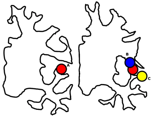
Figure 3.1: Spatial proximity can be a false indicator of correspondence, as illustrated by points lying on opposing sides of a sulcus of the brain. Point A on the left brain is closer to point B on the right brain than it is to point C (AB < AC). However, it is intuitively clear that A is much more likely to correspond to C than to B, as C is located on the opposite bank of the sulcus. A’s position is replicated on the right brain for ease of comparison.
3.2.1
Using Local Features for Generalizing MDL
A natural solution to these issues is to make use of geometric information that goes beyond spatial location, such as local curvature. The MDL objective function can be extended to incorporate such local features, as we presented in [44, 45]. The extension I propose is applicable to not only geometric measures such as curvature, but to any local features whose absolute difference defines a metric in the feature space, as long as the feature values are available at each sample location. Depending on the application domain, appropriate local features might be proximity to major blood vessels, connectivity to other anatomical structures, image intensities, etc.
necessary to substitute the data matrixLencoding the spatial locations in traditional MDL. In this alternative matrix the columns are the local feature values, such as curvature measurements of the object, instead of spatial locations. Therefore, the cost function for MDL must be modified to be based on the eigenvalues of the curvature matrix instead of the eigenvalues of the location matrix.
With this technique, it is possible to use local features that are high dimensional, such as different curvature measurements, or to even include the spatial location itself as a feature dimension, in addition to the other application-driven features.
3.3
Geometric Features
The choice of specific features for representing local shape is one of the issues in using geometrical features to improve MDL. In this section, I review some candidates for local geometrical features. The feature selection will be made based on some of the correspondence evaluation techniques reviewed in Section 2.3, in particular, the generalization and specificity metrics.
3.3.1
Principal Curvatures
(
κ
1, κ
2)
In differential geometry, the second fundamental form II is a quadratic form on the tangent plane of a smooth surface in the 3-D Euclidean space. The second funda-mental form is a symmetric bilinear map that captures the local shape of the surface [18]. In this context, shape is how the surface normal direction changes while mov-ing along the surface in arbitrary directions. The principal directions of the surface can be computed as the eigenvectors of II. The associated eigenvalues of the second fundamental form are called the principal curvatures κ1 and κ2 (chosen such that
κ1 ≥κ2). These values measure the maximum and minimum values of bending of a
3.3.2
Mean Curvature and Gaussian Curvature
(H, K)
The trace and determinant of the second fundamental form capture geometric in-variants regarding the shape of the surface. The mean curvature is defined as H =
1
2(κ1 +κ2) — half the trace of II. Koenderink [18] describes it as “the nosedive
averaged over all directions”, where the ‘nosedive’ refers to the amount of twist-free turning of the principal frame field. Mean curvature is an extrinsic measure of cur-vature.
The Gaussian curvature is the determinant of II, defined as K = κ1κ2. The
Gaussian curvature can be interpreted extrinsically as the measure of the spread of surface normals per unit surface area. This corresponds to the area magnification of the Gauss map, hence the name “Gaussian curvature”. However, K is an intrinsic measure since it is invariant under local isometries and its value can be computed from measurements on the surface itself, regardless of the way the surface is situated in 3D space. This is the result of Gauss’s famous Theorema Egregium [18].
H and K are both algebraic invariants, meaning that they do not change depend-ing on the choice of frame field for the surface, and geometric invariants, meandepend-ing that they do not change when the surface is rotated or translated. However, these measures are not scale-invariant.
3.3.3
Curvedness and Shape Index
(C, S)
Koenderink [18] points out that all spheres intuitively have the same shape even though they may have different sizes. All of the above curvature metrics fail to capture this intuitive property. Koenderink therefore proposes two new metrics to reflect these properties, the curvedness C and the shape index S.
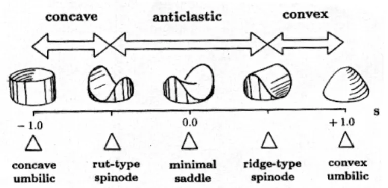
Figure 3.2: Shape index S. The shape index is a curvature-based metric that intu-itively captures local shape. S can take on values from [−1..1]. Shapes with opposite values of S have the relationship of an object and its mold. Figure reprinted from [18].
It is formally defined as:
S =−2
πtan
−1κ1+κ2
κ1−κ2
(3.5)
Figure 3.2 illustrates surfaces corresponding to various values of S. S takes values in the interval [−1..1], with the endpoints corresponding to the concave and convex
umbilics (i.e., points whereκ1 =κ2).
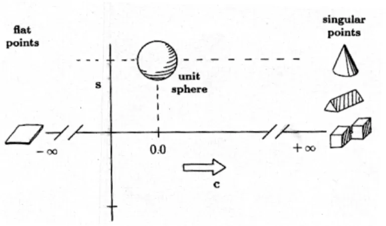
The curvedness C represents how curved the surface is. It is formally defined as:
C = 2
πln
r
κ21+κ22
2 (3.6)
Figure 3.3 illustrates surfaces corresponding to various values of C. C can take any value in (−∞..∞), with −∞corresponding to a flat point and +∞corresponding to
a singular point.
Figure 3.3: Curvedness C. Curvedness captures the size of a surface regardless of its shape. The unit sphere has a C value of 0. Positive values of C correspond to increasingly sharp points, and negative values correspond to increasingly flat surfaces. Figure reprinted from [18].
Section 2.1.1, Tosun et al. [17] use C and S as part of their cortical correspondence scheme.
3.4
Results and Discussion
In this section, I present a practical comparison of four correspondence methods dis-cussed so far: SPHARM correspondence (Sec. 2.1.1), Heimann’s implementation of position-based MDL (Sec. 3.1.2), generalized MDL correspondence (Sec. 3.2) using a pair of curvature measures (denotedCurvMDL) and generalized MDL correspondence using position and a pair of curvature measures (denotedCombinationMDL). Further-more, I have applied the CurvMDL and CombinationMDL methods separately using each pair of metrics discussed in Sec. 3.3.
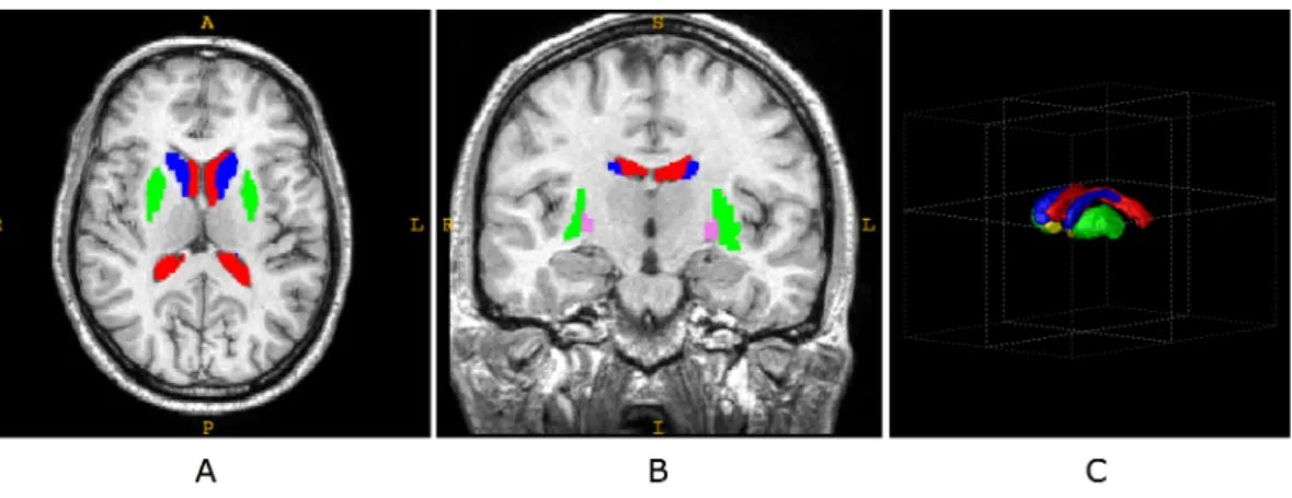
Figure 3.4: The relative locations of the various brain structures used in experiments. Representative axial (A) and coronal (B) slices are shown, as well as a 3D rendering (C). The caudate nuclei, shown in blue, are located near the centre of the brain. The putamen, shown in green, is the outermost part of the basal ganglia. The striatum is the structure comprised of the caudate and the putamen, which are separated by the internal capsule fiber tract, and the nucleus accumbens (shown in yellow). The pallidum, shown in purple in the 2D views, is the other nucleus among the rostral basal ganglia. The lateral ventricles, shown in red, are roughly wrapped around the rostral basal ganglia.
of the brain structures (lateral ventricles, caudates and striata). All populations of brain structures included healthy subjects as well as patients with various disor-ders. This setting leads to a higher variability in the populations. The results of the SPHARM correspondence have been used as initialization to all MDL-based methods, since these require a spherical parameterization for the surface. All curvature mea-sures have been analytically computed from the SPHARM coefficients (see Appendix A for details).
Figure 3.5: The results of the SPHARM, traditional MDL and CombinationMDL demonstrated on two striata and two femoral heads. The coloring shows the φ co-ordinates on the spherical parameterization of the objects, with each (x, y, z) point on the object surface mapped to a (φ, θ) point on the unit sphere. Locations with same coloring on the two subjects correspond to each other for a given method. As shown in (c), the line separating blue and red regions corresponds to a longitude line on the unit sphere. Note that the SPHARM correspondence for the striata is very poor, and the CombinationMDL method gives the best visual correspondence for both populations.
in Figure 3.5, the incorporation of curvature improves the correspondence.
For all populations, the choice of particular pair of curvature measures proved not to be critical, since any of the 3 pairs of measures I used resulted in performances in the same range. This result is not surprising, since given any pair of measures I presented, one can easily compute the other 2 pairs: each pair encodes the same information about the surface shape. To improve graph readability, I only show results using the (C, S) pair of metrics on most of the figures in this chapter.
In the generalized MDL methods (CurvMDL and CombinationMDL), I have scaled the feature values appropriately. This is accomplished by using the inverse of the feature variance averaged over the whole surface as the scaling factor. This forces all feature channels to have a variance of 1 and to therefore have equal weight in the correspondence optimization.
The MDL implementation that I used requires a parameterization mesh as an additional input to determine the spatial resolution at which correspondence opti-mization is performed. In all computations I have used a mesh of the same resolution as the one used for SPHARM computation to obtain full-resolution correspondence. However, one might want to use a lower-resolution parameterization mesh to speed up the computation and interpolate to obtain a denser correspondence. This would lead to a faster but less accurate correspondence optimization.
3.4.1
Lateral Ventricle
The first population consists of 116 lateral ventricle segmentations. These are large, C-shaped structures located in the cerebrum. Shape analysis of the lateral ventricles is important for the study of schizophrenia and Parkinson’s disease [46, 47].
data is similar to adding noise to the dataset. However, the performances of the two methods are still in the same range. Figure 3.6 summarizes these results.
3.4.2
Caudate
The next dataset includes 56 caudate segmentations. The caudate is one of the basal ganglia nuclei, with a vaguely C-shaped geometry with a wide head and a tapering tail. The traditional MDL and the CombinationMDL perform similarly well on this population as expected, given the simple shape of the objects in the population. In fact, Figure 3.7 demonstrates that even SPHARM correspondence performs reasonably well on this dataset, since there are no twists in the structure.
3.4.3
Femur
The third dataset I used consists of 18 truncated femur bones. The femur is a large bone in the upper leg, and its analysis is important to computer assisted surgery as well as prosthesis design [48]. The superior part of the femur has three major protuberances: the head, the greater trochanter and the lesser trochanter. The lower part, including the lower extremity, was truncated and excluded for this study.
For this dataset, due to the complex structure of the objects, the correspondence improves when curvature information is included. Note that, for the generalization metric, traditional MDL catches up with the performance of CombinationMDL when a high number of shape eigenmodes (M) are used. The CombinationMDL has superior specificity values independent of M. Figure 3.8 captures these results.