Maximum Likelihood Estimation for Single Particle, Passive Microrheology Data with Drift John W. R. Mellnik
Curriculum in Bioinformatics and Computational Biology, Department of Mathematics, Department of Biomedical Engineering, University of North Carolina at Chapel Hill, Chapel Hill,
NC 27599, USA
Path BioAnalytics, Inc. Chapel Hill, NC 27510
Martin Lysy
Department of Statistics and Actuarial Science, University of Waterloo, Waterloo, ON N2L 3G1, Canada
Paula A. Vasquez
Department of Mathematics, University of South Carolina, Columbia, SC 29208, USA
Natesh S. Pillai
Department of Statistics, Harvard University, Cambridge, MA 02138, USA
David B. Hill
The Marsico Lung Institute, Department of Physics and Astronomy, University of North Carolina at Chapel Hill, Chapel Hill, NC 27599, USA
Jeremy Cribb
Department of Physics and Astronomy, University of North Carolina at Chapel Hill, Chapel Hill, NC 27599, USA
Scott A. McKinley
Department of Mathematics, Tulane University, New Orleans, LA 70118, USA
M. Gregory Forest
Synopsis
Volume limitations and low yield thresholds of biological fluids have led to widespread use of passive microparticle rheology. The mean-squared-displacement (MSD) statistics of bead position time series (bead paths) are either applied directly to determine the creep compliance [1] or transformed to determine dynamic storage and loss moduli [2]. A prevalent hurdle arises when there is a non-diffusive experimental drift in the data. Commensurate with the
magnitude of drift relative to diffusive mobility, quantified by a Péclet number, the MSD statistics are distorted, and thus the path data must be “corrected” for drift. The standard approach is to estimate and subtract the drift from particle paths, and then calculate MSD statistics. We present an alternative, parametric approach using maximum likelihood
I. INTRODUCTION
The primary application that motivates the methods presented here is the determination of diffusive transport properties and linear viscoelastic properties (dynamic storage and loss moduli or creep compliance) of biological soft matter, and human mucus in particular, based on passive particle tracking microrheology. These viscoelastic inferences arise directly from the mean-squared displacement (MSD) of particle position time series (which we refer to as “paths”). For dynamic moduli, the Mason-Weitz protocol [2, 3, 4] or subsequent corrections [5] are applied to ensemble-averaged transforms of the MSD statistics. The creep compliance follows directly from the time-domain MSD statistics [1]. Video microscopy in combination with passive particle tracking (PPT) has been used to explore the physical properties of a wide range of mucus biogels, including cervicovaginal [6, 7, 8] pulmonary [9, 10] and gastrointestinal [11, 12, 13] mucus. The issue motivating this paper is that often in PPT experiments, the observed particles exhibit drift: a persistent, inadvertent, driven motion potentially due to the light source [10], movement of the optical stage [14, 15], or some other source [16]. We refer to [17] for analysis of static and dynamic errors in PPT data that improve the accuracy of MSD statistics and thereby inferences of material viscoelasticity. For this paper, we restrict ourselves to persistent linear drift over the duration of each particle position time series. Thus the particle observations are a superposition of drift and diffusion. In active biological fluids such as living cells where endogenous DNA domains are fluoresced and tracked, cell translocation and active cellular processes induce additional non-diffusive motion. In viral trafficking within cells, the virus may hijack directed motion along microtubules. Since drift can significantly alter the MSD of tracked particles, and thereby distort the inference of the dynamic moduli or compliance as well as distort the inferred diffusive mobility, the question naturally arises as to how drift should be accounted for in the analysis of PPT data.
Brownian and fractional Brownian motion. The reader is referred to a large body of work by Klafter, Metzler, Barkai and collaborators on fractional Brownian motion as well as other sub- and super-diffusive stochastic processes; see the review article by [20]. In [21] a de-trending method is applied to a larger class of diffusive and sub-diffusive processes with drift in two space dimensions, where the full 2d observations are used to simultaneously estimate the diffusive or sub-diffusive model parameters and the drift. The present article aims to introduce and illustrate the parametric, maximum likelihood estimation approach in one-dimensional PPT data; for a more rigorous treatment, including comparisons of competitive models on the basis of the available data, see [21].
We point out that the debate over the optimal way to remove drifttacitly assumes that directed motion must be removedprior to analyzing the path data. Historically, this assumption is natural because of the focus on the scaling of the ensemble particle MSD due to purely diffusive dynamics [22, 23, 24, 25], a statistic that can be extremely sensitive to drift [26]. In this article, we take a different approach and show that deterministic drift does not need to be removed a priori from particle path data to determine the MSD statistics if one posits and exploits a fully parametric statistical model for the underlying drift-diffusion process. In particular, we focus on fractional Brownian motion (fBm), a parametric statistical model for sub-diffusive processes that has been shown to accurately describe diffusion in mucus gels [9, 21] and other biological soft matter [27, 28]. For other systems where the particle paths do not exhibit relatively uniform power law MSD behavior, our current methods would not be applicable. We are currently considering extensions of our parametric statistical model to other candidate sub-diffusive stochastic models, e.g., generalized Langevin equations that resolve transient sub-diffusion and convergence at long times to normal diffusion. Other types of path properties, such as jumps between different modes of diffusion within a single tracked path, remain for future development.
Using numerical simulations of drift coupled with sub-diffusive fractional Brownian motion (consistent with data from mucus gels), we show that one can easily and accurately estimate the diffusive or sub-diffusive model parameters by maximum likelihood estimation (𝑀𝐿𝐸) -- for a wide range of deterministic drift, and without removing the drift a priori as is typically done to estimate the MSD statistics of single or ensemble paths. The advantage of 𝑀𝐿𝐸 arises because drift is treated as a model parameter to be estimated jointly with the diffusive or sub-diffusive parameters rather than sequentially, thereby increasing the precision of all parameter estimates. With all parameters thus estimated jointly, it is then straightforward to use fBm parameter estimates to generate the MSD of the purely diffusive dynamics and thereby infer the dynamic viscoelastic moduli or the creep compliance. We illustrate the procedure for a range of Péclet numbers, which we define through a dimensionless ratio of the drift (advection) component relative to the diffusive mobility, for both normal and sub-diffusive processes.
can be directly measured and compared to any other method. We are thus able to compare the errors in the inference of diffusive process parameters and drift, in dynamic storage and loss moduli, and in creep compliance, among our proposed parametric maximum likelihood estimation method and the standard approach in the passive microrheology literature (based on a least-squares estimate of the MSD after removal of drift). We also show, for posterity, the dramatic errors in the diffusion parameters and viscoelastic properties if one simply ignores the presence of drift. Finally, for experimental illustration purposes, we apply the 𝑀𝐿𝐸 and standard drift-subtracted MSD estimate approaches to PPT data from human bronchial epithelial cell culture mucus.
The structure of the article is as follows. First, we discuss drawbacks of MSD-based approaches and cursory drift removal. We then introduce a canonical model (fractional Brownian motion) for tunable particle diffusion or sub-diffusion with drift, and provide details on how to simulate particle paths in accordance with this model. Next, we review MSD-based approaches to the recovery of diffusive parameters and present our 𝑀𝐿𝐸 method. The methods are then compared using simulated data sets for a practical range of Péclet numbers. Finally we illustrate the methods on data from human lung cell culture mucus.
II. MEAN SQUARED DISPLACEMENT STATISTICS
Given (𝑀 + 1) observations 𝑋(0), 𝑋(∆𝑡), 𝑋(2∆𝑡), … , 𝑋(𝑀∆𝑡) of a particle’s position, the MSD statistic is calculated as
〈𝑟𝜏𝑖〉2 = 1
𝑀 − 𝑖 + 1∑[𝑋(𝜏𝑖 + 𝑗∆𝑡) − 𝑋(𝑗∆𝑡)]2, 𝑀−𝑖
𝑗=0 (1)
where 𝜏𝑖 = 𝑖∆𝑡 is called the lag time and ∆𝑡 is the time between observations. Note that for larger lag times, the number of observations decreases, limiting the statistical significance of the MSD. For many diffusive processes, theory and observation suggest that the MSD of particles undergoing diffusion exhibits a power law scaling over a range of lag times for which there are sufficient observations [29, 6, 4, 30, 31, 9]:
𝐸[〈𝑟𝜏〉2] = 2𝑑𝐷𝜏𝛼, (2)
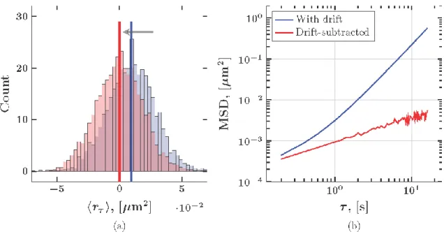
versus lag time 𝜏 to tend toward a slope of 2 at large lag times (Figure 1). That is, as 𝜏 increases,
𝛼 → 2 and the larger the drift velocity, the smaller the lag time at which this transition occurs.
Figure 1: Path-wise MSD for simulated particles from the Brownian motion (Bm) (a) and fractional Brownian motion (fBm) (b). MSD curves for 40 representative data sets are shown for varying drift characterized by the Péclet number (Pe), the ratio of the advective and diffusive transport rates (Eqn. (13)). The color scheme represents increasing Péclet from 𝑃𝑒𝑚𝑖𝑛 = 0 (blue) to 𝑃𝑒𝑚𝑎𝑥= 0.73 (red), for the Bm data set, and from 𝑃𝑒𝑚𝑖𝑛= 0 (blue) to 𝑃𝑒𝑚𝑎𝑥 = 0.52 (red) for the fBm data set. The upper and lower black dashed lines indicate slopes of 2 (ballistic motion) and 1 (normal diffusion), respectively. The fBm paths (b) are simulated with 𝛼 = 0.6; the "diffusivity" pre-factor is chosen to have the same numerical value in the two data sets.
When one attempts pathwise correction for directed motion by subtracting the mean increment from each path, i.e., the mean of the step-size distribution at the shortest lag time (Figure 2), one inadvertently changes the structure of the entire particle path. That is, every such modified path is constrained to begin and end at the same spatial position. To see this, consider a one-dimensional Brownian path, where 𝑋𝑖 = 𝑋(𝑖∆𝑡) is the location of the particle at time 𝑖∆𝑡 with 𝑖 = 1, 2, 3 … 𝑀. The increments of this process are given by
𝑥𝑖 = 𝑋𝑖+1− 𝑋𝑖. (3)
𝑥̅ = 1
𝑀 − 1 ∑ 𝑥𝑖 𝑀−1
𝑖=1
, (4)
converges to zero as the number of particle positions increases, i.e. as 𝑀 → ∞. The fact that the distribution of 𝑥𝑖 is symmetric with 𝑥̅ converging to zero intuitively indicates that the particle is expected to make an equal number of steps to the left and right. This however, is not to say that a particle diffusing via Brownian motion never travels a net distance. The mean incremental displacement is 𝑥̅, and when we subtract 𝑥̅ from each increment, 𝑥𝑖, we “snap” the distribution of 𝑋𝑀 to zero, inadvertently stipulating that the first and final positions of the particle are the same. Indeed, suppose that 𝑥̅ is subtracted from each increment to “remove drift,” centering the distribution of increments at zero. The resulting modified position process is computed by taking the cumulative sum of the shifted increments, denoted by 𝑋̃𝑖,
𝑋̃1 = 𝑋1
𝑋̃2 = 𝑋1+ (𝑥1− 𝑥̅)
𝑋̃3 = 𝑋1+ (𝑥1− 𝑥̅) + (𝑥2− 𝑥̅)
𝑋̃4 = 𝑋1+ (𝑥1− 𝑥̅) + (𝑥2− 𝑥̅) + (𝑥3− 𝑥̅) ⋮
(5)
Following this pattern, we collect terms and write the final position 𝑋̃𝑀 as,
𝑋̃𝑀 = 𝑋1− (𝑀 − 1)𝑥̅ + ∑ 𝑥𝑖, 𝑀−1
𝑖=1
(6)
which can be simplified further,
𝑋̃𝑀 = 𝑋1− (𝑀 − 1) 1
𝑀 − 1∑ 𝑥𝑖 𝑀−1
𝑖=1
+ ∑ 𝑥𝑖 𝑀−1
𝑖=1 (7)
𝑋̃𝑀 = 𝑋1− ∑ 𝑥𝑖 𝑀−1
𝑖=1
+ ∑ 𝑥𝑖 𝑀−1
𝑖=1 (8)
𝑋̃𝑀 = 𝑋1 (9)
procedure if the paths are from a standard Brownian motion (because the increments are independent), it becomes relevant when the paths are from any stochastic process where the increments may be highly correlated, and in particular, sub-diffusive processes typical of biogels. An additional drawback of an MSD-based approach to diffusive parameter estimation is the unreliability in the MSD at large lag times. As the lag time increases, the number of increments included in the mean of the squared increments decreases and thus becomes less stable. [26] estimate that only the initial two-thirds of the MSD is statistically reliable. Due to experimental factors (particles exiting the focal plane of the microscope) limiting the ability to collect data over long time scales, the uncertainty in the MSD for large lag times can have a pronounced impact on the accurate recovery of diffusive and viscoelastic properties.
Figure 2: Impact of drift-subtraction on the distribution of increments and MSD for a representative sub-diffusive fractional Brownian motion path with true parameter values 𝛼 = 0.60 and 𝐷 = 4.67 × 10⁻⁴ 𝜇𝑚2𝑠−𝛼. The estimated parameter values based on a simple least-squares fit to the drift subtracted MSD are 𝛼 = 0.53 and D =
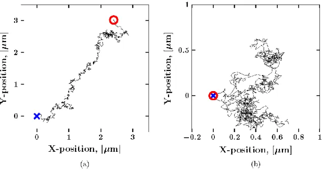
Figure 3: Sample Brownian path with drift (a) and after the drift has been removed by subtracting the mean displacement from each increment (b). The beginning and end of the path have been marked with a blue x and a red circle, respectively.
III. FRACTIONAL BROWNIAN MOTION AND DRIFT
Recently, [21] considered fractional Brownian motion (fBm) as a model for the movement of micron-scale particles over a 30 second observation time at 60 frames per second temporal resolution in human bronchial epithelial mucus. Under this model, the particle's position process
𝑋(𝑡) in one dimension is written as the sum of a deterministic term representing the drift and a stochastic term representing the particle’s thermally activated diffusive movements:
𝑋(𝑡) = 𝜇𝑡 + √2𝐷𝑊𝛼(𝑡), (10)
where 𝑊𝛼(𝑡) is acontinuous Gaussian process with mean zero and covariance
𝑐𝑜𝑣[𝑊𝛼(𝑡), 𝑊𝛼(𝑠)] = 12(|𝑡|𝛼+ |𝑠|𝛼− |𝑡 − 𝑠|𝛼), 0 < 𝛼 < 2. (11)
𝑐𝑜𝑣[𝑥𝑖, 𝑥𝑖+𝑘] = 𝐷∆𝑡𝛼(|𝑘 + 1|𝛼+ |𝑘 − 1|𝛼− 2|𝑘|𝛼). (12)
For fBm processes, the MSD has the same scaling relation as Brownian motion [33], i.e.,
〈𝑟𝜏〉2~𝐷𝜏𝛼, although, unlike Brownian motion, the power-law exponent is not necessarily unity. When 𝛼 < 1, the fBm increments are negatively correlated and the position process exhibits subdiffusive behavior. When 𝛼 > 1, the fBm increments are positively correlated and the position process exhibits superdiffusive behavior.
Calculating the increments 𝑥𝑖 provides a simple way to estimate the drift exhibited by a particle since the mean, or expected value 𝐸[… ], of the increments is 𝐸[𝑥𝑖] = 𝜇∆𝑡, for both Brownian and fractional Brownian processes. To generalize our analysis, we characterize results in terms of a Péclet number (𝑃𝑒), a dimensionless ratio of the advective and diffusive transport rates. Given the increments of a particle path computed for a given lag time ∆𝑡, we introduce an approximate Péclet number that is derived directly from the data collected in drift-diffusion microrheology experiments where one does not a priori know either the fluid velocity or the fluid diffusivity, and furthermore where fractional diffusivities arise. Namely, at the observation timescale (∆𝑡 = 1/60 s), from the observed data, we define an approximate Péclet number as the ratio of the mean increment of the particle path, 𝐸[𝑥𝑖] or the expected value of 𝑥𝑖, and the standard deviation 𝑆𝐷[𝑥𝑖] of the increments,
𝑃𝑒 ≡ 𝐸[𝑥𝑖]
𝑆𝐷[𝑥𝑖]. (13)
This definition is not a "pure" Péclet number for all particle tracking experiments. The numerator includes a lower order contribution from apparent diffusive drift due to a finite number of observations. The denominator will include the standard deviation in the advection process if the drift per increment is not identical (due to non-constant drift or measurement error). Nonetheless, this is a reasonable Péclet number based purely on the data, which one could correct later from the results of the MLE method. (GF thanks Ian Seim for a discussion of this issue.)
IV.A METHODS: Simulation
To generate a particle path exhibiting linear drift and fractional or normal Brownian dynamics, we first generate the increment process for an fBm path without drift, and then add the desired drift to the path. To generate fBm observations 𝑋1,…, 𝑋𝑀 for a particular choice of 𝛼, we first construct the covariance matrix 𝑺of the increment process according to Eqn. (12). That is, the
𝑺𝑖,𝑗= 𝑐𝑜𝑣[𝑥𝑖, 𝑥𝑗] (14)
for 𝑖, 𝑗 = 1, 2, … 𝑀. Let 𝑳𝑳′= 𝑺be the Cholesky decomposition of 𝑺 and let 𝒖 be a vector of M independent and identically distributed draws from a standard normal distribution. A simulated particle path is generated as 𝒙 = (𝑥1, … , 𝑥𝑀)′= √2𝐷𝑳𝒖, 𝑋𝑗 = ∑𝑗𝑖=1𝑥𝑖. Using this method, two sets of simulated data are generated. The first set is subdiffusive with 𝛼 = 0.6 and 𝐷 = 4.67 ×
10−4 μm2s−α, mimicking the estimated parameter values based on experimental observations of 1 μm diameter particles in 4 weight percent human bronchial epithelial mucus [9]. The second data set exhibits standard Brownian motion, i.e., 𝛼 = 1, with diffusivity 𝐷 = 4.67 ×
10−4 μm2s−1 corresponding to a 1 μm diameter particle in a fluid with viscosity of 1.86 Pa s at 23 °C. Each simulated path is generated with a temporal resolution of 5 frames per second and a length of 𝑀 = 2,992 steps, mimicking experimental conditions for the experimental data presented in Section VII.
Linear drift is added to the simulated paths by calculating the increments, adding directed motion, then taking the cumulative sum of the result. We simulate both fractional and normal diffusive paths for Péclet numbers in the range [0, 0.73] for Brownian motion and [0, 0.52] for fractional Brownian motion, chosen such that we match the range of drift relative to diffusion as defined by Eqn. (13) for the observed experimental data (Section VII). A position process with linear drift is given by,
𝑋𝑗 = ∑(𝑥𝑖 𝑗
𝑖=1
+ 𝛬), (15)
where 𝛬 is a scaling factor with units of μm. We generate 100 simulated paths with drift for 𝛬 spanning the interval [0, 9.34 × 10⁻³] in increments of 2.3 × 10⁻⁴ μm, resulting in 4,100 simulated fBm paths (𝛼 = 0.6) and 4,100 simulated Brownian paths (𝛼 = 1). These data sets will be referred to as the fractional Brownian motion (fBm) and Brownian motion (Bm) data sets, respectively.
IV.B METHODS: Experimental
the composition of mucus harvested from HBE cultures is highly conversed with human sputum [38] and reproduces the osmotic pressure [39] and rheological properties of sputum [9]. Physiologically, HBE mucus has been used to ascertain the role of mucus concentration in pathological bacterial biofilm formation [36], reduced neutrophil activity and motility [35], and clearance [40]. Finally, the concentration of HBE mucus, a simple biochemical property of mucus, has been shown to be correlated with disease states and severity [36, 39, 9, 40].
We selected 1 μm diameter polystyrene particles with carboxyl surface chemistry (Fluospheres, Fisher Scientific) for use in our assays. This particle size is substantially larger than the length scales of the mucin mesh network [41, 42, 43, 44, 9]. Further, the carboxyl functionalization rather than an amine surface chemistry was chosen as previous studies have shown that amine treated beads have impaired diffusion in sputum [45]. PEG surface chemistries, which enhance the diffusion of smaller particles (200 nm and smaller) [41, 46] in mucus have little effect on the diffusivity of larger (>500 nm diameter) particles [46]. These factors lead us to use 1 μm diameter particles with carboxylic acid functionalization. Particles of this size will more faithfully mimic linear macroscopic rheology [43, 47]. Further, by using HBE mucus prepared to concentrations prescribed by physiologically relevant states, we are able to avoid the 100 fold variations in reported literature values that were evident in earlier mucus macroscopic assays [48].
V. APPROACHES TO PARAMETER ESTIMATION
We consider three approaches to diffusive parameter estimation.
Simple least squares Noting that the subdiffusive MSD is linear on the log-log scale,
ln(𝐸[〈𝑟𝜏〉𝑖2]) = ln(2𝐷) + 𝛼ln(𝜏𝑖), (16)
a longstanding approach to estimate 𝐷 and 𝛼 is to minimize the least squares (𝐿𝑆) objective function
∑𝑀 (𝑦𝑖 − 𝑐 − 𝛼𝑡𝑖)2
𝑖=1 , (17)
in terms of 𝑐 and 𝛼 where,
𝑦𝑖 = ln[〈𝑟𝜏〉𝑖2], c = ln[2𝐷], 𝑡𝑖 = ln[𝜏𝑖]. (18)
Recall that 𝑀 is the number of particle positions. The minimum of Eqn. (17) is obtained at 𝛼̃ =
∑𝑀 𝑦𝑖𝑡𝑖
Drift-Subtracted Least Squares The drift-subtracted least squares (𝐷𝐿𝑆) approach subtracts 𝑥̅, the mean increment (Eqn. (4)), from each 𝑥𝑖 (Eqn. (3)), centering the distribution of increments at zero, dictating the equivalence of the initial and final position, before applying the approach described above for least squares estimation.
Full Model MLE This approach applies maximum likelihood estimation (𝑀𝐿𝐸) to Eqn. (10) to estimate 𝜇, 𝐷 and 𝛼 directly from the raw data without first estimating the MSD statistic. The fBm model in Eqn. (10) specifies that the increments 𝒙 = (𝑥1, … , 𝑥𝑀)′ have a multivariate Gaussian distribution with mean 𝐸[𝑥𝑖] = 𝜇Δ𝑡 and variance matrix 𝑺 given by Eqn. (14), denoted
𝒙~𝒩(𝜇∆𝑡, 𝑺). (19)
Let 𝑺 = 𝜎2𝑽𝛼, where 𝜎 = 2𝐷 and 𝑽𝛼 is a matrix independent of 𝐷. The likelihood of a set of model parameters 𝜽 = (𝜇, 𝜎, 𝛼), given a set of observations 𝒙, is given by the likelihood function
ℒ(𝜽|𝒙) = exp [−1 2
(𝒙 − 𝜇∆𝑡)′𝑽 𝛼
−1(𝒙 − 𝜇∆𝑡)
𝜎2 −
1
2ln(|𝜎2𝑽𝛼|)], (20)
which, up to a factor of (2𝜋)−𝑀 2⁄ , is the probability density function (PDF) of the multivariate Gaussian specified by Eqn. (19). The 𝑀𝐿𝐸 of the parameters is
𝜽̂ = argmax𝜽ℒ(𝜽|𝒙), (21)
the value of 𝜽 that maximizes ℒ(𝜽|𝒙). The three-dimensional optimization problem in Eqn. (21) can be reduced to a one-dimensional problem by maximizing in (𝜇, 𝜎) for fixed 𝛼. That is, let
𝒚 = 𝒚𝛼 = [𝑽𝛼]−1/2𝒙, and 𝒛 = 𝒛
𝛼 = ∆𝑡[𝑽𝛼]−1/2𝟏𝑀, (22)
where 𝟏𝑀 = (1, 1, … 1)′. Then the 𝒚 = (𝑦1, … 𝑦𝑀)′ are independent Gaussians with common variance 𝜎2, so that
𝑦𝑖 𝑖𝑛𝑑∼ 𝒩(𝜇𝑧
𝑖, 𝜎2), (23)
such that for fixed 𝛼, the two-parameter likelihood function ℒ𝛼(𝜇, 𝜎|𝒙) is
ℒ𝛼(𝜇, 𝜎|𝒙) = exp [−Mln(σ) − ∑
(𝑦𝑖− 𝜇𝑧𝑖)2 2𝜎2 𝑀
𝑖=1 ]. (24)
𝜇̂𝛼= ∑ 𝑧𝑖𝑦𝑖 𝑀 𝑖=1 ∑𝑀 𝑧𝑖2
𝑖=1
, 𝜎̂𝛼= (∑𝑀𝑖=1(𝑦𝑖 − 𝜇̂𝛼𝑧𝑖)2
𝑀 )
1/2
. (25)
The 𝑀𝐿𝐸 of 𝛼 for Eqn. (10) is thus obtained by maximizing the one-dimensional profile likelihood function [49]
ℒprof(𝛼|𝒙) ≝ ℒ(𝜇̂𝛼, 𝜎̂𝛼, 𝛼|𝒙). (26)
Specifically, by substituting Eqn. (25) into Eqn. (24), we find the 𝛼̂ that maximizes
ℓprof(𝛼|𝒙) = ln (ℒprof(𝛼|𝒙)) + 𝐶
= −1
2[𝑀ln(𝜎̂𝛼2) + ln(|𝑽𝛼|)].
(27)
(28)
The resulting parameter estimates 𝜃̂ = (𝜇̂𝛼̂, 𝛼̂, 𝜎̂𝛼̂) are precisely those that maximize the full likelihood ℒ(𝜃|𝑥), thereby reducing the numerical optimization problem from three parameters to one. Moreover, we note that for arbitrary variance matrix 𝑽, the linear systems in Eqn. (22) are solved in 𝑂(𝑀3) operations. However, since 𝑽𝛼 is a Toeplitz matrix [50], the systems can be solved in 𝑂(𝑀2) operations using the Durbin-Levinson algorithm [51, 52].
The 𝑀𝐿𝐸 was implemented in MATLAB, except the Durbin-Levinson algorithm which was implemented in C++. While the DLS estimate is much faster to compute, both algorithms scale as 𝑂(𝑀2). For 2-d paths of length 𝑀 = 3000, 5000, 10000, each 𝑀𝐿𝐸 took 0.3, 0.8, 3.3 seconds to evaluate on a personal computer. Pseudocode for the 𝑀𝐿𝐸 of fBm with drift can be found in Appendix A.
Much like the least squares approach involving the sample MSD, the maximum likelihood approach we have described hinges on the minimization of a quadratic objective function. However, whereas the least squares approach estimates the drift only once, the 𝑀𝐿𝐸 estimates the "optimal" drift and diffusivity for every value of 𝛼. That is, the least squares estimate of the drift by 𝑥̅ would be optimal if the increments were uncorrelated, whereas the 𝑀𝐿𝐸 approach estimates the drift by a weighted average of the increments, 𝜇̂𝛼 that accounts for their correlation. Indeed, 𝜇̂𝛼 = 𝑥̅ only when fBm reduces to ordinary diffusion with 𝛼 = 1.
VI.A. RESULTS: Simulated Data
𝐺∗(𝜔) = 𝑖𝜔𝜂∗(𝜔) = 𝐺′(𝜔) + 𝑖𝐺′′(𝜔) = 𝑘𝐵𝑇
𝜋𝑎𝑖𝜔𝔉{〈𝑟𝜏〉2}, (29)
where 𝔉{𝑔(𝜏)} = ∫ 𝑔(𝜏)𝑒−𝜔𝑖⋅𝜏𝑑𝜏 denotes the Fourier transform. Note, the dynamic viscosity
𝜂′(𝜔) is related to the viscous modulus via 𝜔𝜂′(𝜔) = 𝐺′′(𝜔). We note further that for fBM and our experimental data, the MSD curves are highly uniform. For data where the MSD curves are non-uniform, corrections to (20) should be used, cf. [5].
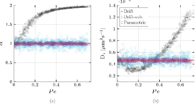
Figure 4: Estimated values of 𝛼 (a) and 𝐷 (b) ignoring drift (black circles), subtracting drift (blue circles) and our maximum likelihood method (violet circles). The true values of 𝛼 and 𝐷 are shown in solid red lines. The true values of each parameter are 𝛼 = 1 and 𝐷 = 4.67 × 10⁻⁴ 𝜇𝑚2𝑠−1.
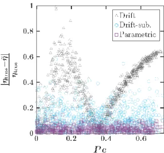
Figure 5: Relative error in estimates of the viscosity (𝜂) given by the Stokes-Einstein relation based on the three approaches for the Brownian motion data set as a function of the Péclet number (Pe). The mean error in the estimation of 𝜂 when not accounting for drift is 39.5%. When applying a drift-subtracted least squares approach and a parametric approach the mean error is 11.1% and 3.6%, respectively.
Figure 6 illustrates the impact of drift on the pathwise estimates of 𝐺′ and 𝐺′′ for the fBm data for various values of 𝑃𝑒. In Figure 7, the ensemble average estimates 𝐺′ and 𝐺′′ are compared when applying Eqn. (29) to the empirical MSD when ignoring drift and subtracting drift, and applying Eqn. (29) to the parametric scaling of the MSD predicted by our 𝑀𝐿𝐸 approach for 𝛬 =
9.34 × 10⁻³ μm, corresponding to 𝑃𝑒 = [0.48, 0.52] for the fBm data. The ensemble average relative error in the estimation of 𝐺′ and 𝐺′′ for the fBm data set is reported for the 𝐷𝐿𝑆 and
Figure 6: Pathwise dynamic storage, 𝐺′(𝜔) (a), and loss, 𝐺′′(𝜔) (b) moduli for the fBm data found by transforming the pathwise MSD without accounting for drift. The change in color of the data corresponds to a transition from
𝑃𝑒𝑚𝑖𝑛 = 0 (blue) to 𝑃𝑒𝑚𝑎𝑥= 0.52 (red). The true values of 𝐺′and 𝐺′′are indicated by the black dashed lines.
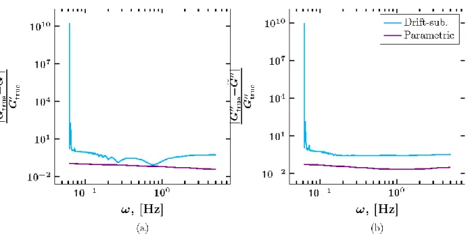
Figure 8: Ensemble averaged relative error in the storage modulus, 𝐺′(𝜔) (a), and loss modulus, 𝐺′′(𝜔) (b) for the fBm data with subdiffusive exponent 𝛼 = 0.6 when applying Eqn. (29) to the empirical MSD after subtracting drift (blue) and applying Eqn. (29) to the parametric scaling of the MSD predicted by our maximum likelihood method (violet). The ensemble average is computed using all 4,100 simulated paths.
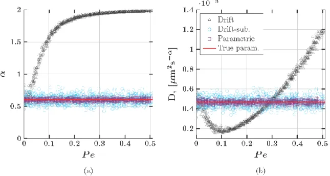
Figure 9: Estimated values of 𝛼 (a) and 𝐷 (b) ignoring drift (black circles), subtracting drift (blue circles) and our maximum likelihood method (violet circles). The true values of 𝛼 and 𝐷 are shown in solid red lines. The true values of each parameter are 𝛼 = 0.6 and 𝐷 = 4.67 × 10⁻⁴ 𝜇𝑚2𝑠−𝛼.
VI.B. RESULTS: Experimental Data
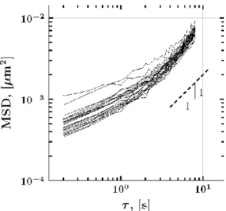
Here, we analyze twenty-two representative 1 μm diameter particles in 4 weight percent human bronchial epithelial (HBE) mucus using the previously outlined methods. Each path consists of 2,992 increments with a temporal resolution of 0.2 seconds (five observations per second). The MSD for each experimental path is shown in Figure 10. The ensemble-averaged storage and loss moduli are calculated when ignoring drift, subtracting drift by applying Eqn. (29) to the empirical MSD, and applying Eqn. (29) to the parametric scaling of the MSD of the pure fBm process determined from our maximum likelihood method (Figure 11).
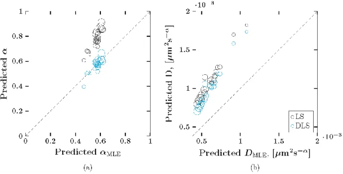
The three estimation methods for 𝐷 and 𝛼 were applied to the experimental particle paths. Figure 12 shows the least squares (𝐿𝑆) and drift-subtracted least squares (𝐷𝐿𝑆) estimates relative to the full model maximum likelihood estimation approach (𝑀𝐿𝐸). The estimates for 𝛼 are presented in Figure 12a. The 𝑀𝐿𝐸 predictions of 𝛼 are shown along the x-axis and the 𝐿𝑆 and
indicates that the 𝐿𝑆 (or 𝐷𝐿𝑆) approach underestimated𝛼 compared to the 𝑀𝐿𝐸 approach. The size of each data point is directly proportional to the calculated drift for the corresponding particle.
Figure 10: Path-wise MSD for the 22 experimental particle paths. The dashed line indicates a slope of 1, corresponding to normal diffusion.
In Figure 12a, the 𝐷𝐿𝑆 and 𝑀𝐿𝐸 approaches exhibit strong agreement in their predictions of 𝛼, as evidenced by the distribution of data points (blue) along the diagonal dashed line. In contrast, the 𝐿𝑆 estimates of 𝛼 (black) fall above the diagonal, indicating an overestimation of 𝛼 relative to the 𝑀𝐿𝐸 approach. The amount of overestimation is directly proportional to the amount of drift in the experimental data (larger markers are further from the diagonal than smaller markers).
Figure 12b presents the estimates of the diffusivity (𝐷). All data points fall above the diagonal, thus both the 𝐿𝑆 and 𝐷𝐿𝑆 approach estimate larger values of 𝐷 compared with the 𝑀𝐿𝐸 approach. Here, the amount of overestimation is inversely proportional to the amount of drift (larger markers are closer to the diagonal). We note that this is not a scenario observed in the simulated data. Returning to Figure 9, we see that the only time the 𝐿𝑆 estimates of 𝐷 are in increasing correspondence to the 𝑀𝐿𝐸 values with increasing drift is when the 𝐿𝑆 method underestimates 𝐷 and 0.1 < 𝑃𝑒 < 0.3. Furthermore, according to Figure 9, the 𝐷𝐿𝑆 estimate of
𝐷 relative to the 𝑀𝐿𝐸 values should be independent of 𝑃𝑒. We hypothesize that these incongruences between the simulated and experimental data may be the result of non-linear drift, an interesting issue but beyond the scope of the present paper.
VII. DISCUSSION
Persistent linear drift over the course of a particle path is compounded at large lag times, resulting in an asymptotic (long lag time) bending of the MSD curve toward a slope of 2. The use of MSD curves for inference of mobility, creep compliance, or linear viscoelastic moduli, without recognizing there is drift and accounting for it, is obviously problematic. We use a simple calculation of the mean and standard deviation of the step size distribution for a given experimental or numerical particle path to estimate the drift relative to diffusion, defining an approximate Péclet number 𝑃𝑒.
When 𝑃𝑒 increases, the slope of the path-wise MSD approaches 2 at increasingly smaller lag times, causing the least squares (𝐿𝑆) estimate of the power law exponent, 𝛼, to converge to 2. By subtracting the mean increment of each particle from the particle’s path, the least squares (𝐷𝐿𝑆) estimate of each parameter is more stable. However, the unanticipated correlation in the increment process induced by drift subtraction over increasingly large lag times leads to an error in the estimation of the diffusive parameters that is on the order of 10%. Accordingly, these discrepancies at large lag times produce errors in creep compliance at those lag times and in the dynamic moduli at low frequencies.
To address this issue, we advocate for a parametric maximum likelihood estimation (𝑀𝐿𝐸) approach that identifies the best-fit drift parameter 𝜇 simultaneously while estimating 𝐷 and 𝛼. We demonstrate on numerically generated particle paths, with physically relevant diffusive parameters from human bronchial epithelial mucus studies, that the use of the parametric maximum likelihood approach results in approximately a 2/3 reduction in the error in the exact fractional Brownian motion parameters 𝐷 and 𝛼 compared to the standard drift-subtraction least squares approach. Such diffusive mobility parameters are routinely used in drug delivery to compare various drug delivery particle formulations for passage through mucosal layers [7, 8, 10]. With respect to inference of linear viscoelasticity from the MSD statistics of particle paths, we have illustrated that accuracy in storage and loss moduli deteriorates at low frequencies for the standard drift-subtraction, least squares methods. The gains in accuracy by the 𝑀𝐿𝐸 method have been shown for fractional Brownian numerical data typical of experimentally observed data in mucus gels. Furthermore, we note that the statistical properties of the 𝑀𝐿𝐸 method are well understood in the statistics community, and have further value beyond that illustrated here, e.g., for testing model assumptions against experimental data as in [21].
linear response (unpublished data) make this macro-micro rheology comparison more intricate than for other systems such as actin filament networks [1].
VII. ACKNOWLEDGEMENTS
The authors gratefully acknowledge partial support from the National Science Foundation Grants DMS-1412844, DMS-1100281, DMS-1462992, DMS-1412998, DMS-1410047, DMS-1107070, National Institutes of Health and National Heart Lung and Blood Institute grants NIH/NHLBI 1 P01 HL108808-01A1, NIH/NHLBI 5 R01 HL 077546-05, and Natural Sciences and Engineering Research Council of Canada grant RGPIN-2014-04225.
Appendix. Pseudocode for MLE of fBM with Drift
Instructions:
1. For a given set of observations 𝑿 = (𝑋0, … , 𝑋𝑀) with 𝑋𝑖 = 𝑋(𝑖Δ𝑡), calculate the increments 𝒙 = (𝑥1, … 𝑥𝑀), 𝑥𝑖 = 𝑥𝑖 − 𝑥𝑖−1.
2. For given 𝒙 and Δ𝑡, maximize the function PROFLOGLIK(𝛼, 𝒙, Δ𝑡) as a function of α. For fBM, we have 0 < 𝛼 < 2, so the maximum can easily be obtained using the fminbnd routine in MATLAB.
3. Once we have the MLE 𝛼̂ of 𝛼, we can find the MLEs of 𝜇 and 𝜎2 with {𝜇̂, 𝜎̂2} =MLE(𝛼̂, 𝒙, Δ𝑡).
Evaluate ℓprof(𝛼|𝒙)
𝐟𝐮𝐧𝐜𝐭𝐢𝐨𝐧 PROFLOGLIK(𝛼, 𝒙, Δ𝑡)
𝑀 ← 𝐥𝐞𝐧𝐠𝐭𝐡(𝒙)
{𝜇̂𝛼, 𝜎̂𝛼2, 𝜈} ← MLE(𝛼, 𝒙, Δ𝑡)
𝜆 ← −12(𝑀ln(𝜎̂𝛼2) + 𝜈)
𝐫𝐞𝐭𝐮𝐫𝐧 𝜆
Calculate the MLEs 𝜇̂𝛼 and 𝜎̂𝛼2, as well as 𝜈 = ln(|𝑽𝛼|) 𝐟𝐮𝐧𝐜𝐭𝐢𝐨𝐧 MLE(𝛼, 𝒙, Δ𝑡)
𝜸𝑀×1 ←ACF(𝛼, Δ𝑡, 𝑀)
𝑨2×𝑀 ← [𝑥Δ𝑡 ⋯ Δ𝑡]1 ⋯ 𝑥𝑀
{𝑸2×2, 𝜈} ← DURBINLEVINSON(𝜸, 𝑨) 𝜇̂𝛼 ← 𝑄12/𝑄22
𝜎̂𝛼2 ← 1
𝑀(𝑄11− 𝑄12𝜇̂𝛼) 𝐫𝐞𝐭𝐮𝐫𝐧 {𝜇̂𝛼, 𝜎̂𝛼2, 𝜈}
𝐞𝐧𝐝 𝐟𝐮𝐧𝐜𝐭𝐢𝐨𝐧
Autocorrelation of fBm increments
𝐟𝐮𝐧𝐜𝐭𝐢𝐨𝐧 ACF(𝛼, Δ𝑡, 𝑀)
𝜸𝑀×1 ← 𝟎𝑀×1
𝐟𝐨𝐫 𝑖 ← 1: 𝑀 𝐝𝐨
𝛾𝑖 ←12Δ𝑡𝛼(|𝑖 + 1|𝛼+ |𝑖 − 1|𝛼− 2|𝑖|𝛼)
𝐞𝐧𝐝 𝐟𝐨𝐫
𝐫𝐞𝐭𝐮𝐫𝐧 𝜸
Calculate 𝑸 = 𝑨𝑽−1𝑨′ and 𝜈 = ln(|𝑽|), where 𝑽 = TOEPLITZ(𝜸) 𝐟𝐮𝐧𝐜𝐭𝐢𝐨𝐧 DURBINLEVINSON(𝜸, 𝑨)
{𝑑, 𝑀} ← 𝐝𝐢𝐦𝐬(𝐴𝑑×𝑀) 𝜈 ← 0
𝑸𝑑×𝑑 ← 𝟎𝑑×𝑑
𝝋𝑀×1 ← 𝟎𝑀×1 𝜏 ← 𝛾1
𝐟𝐨𝐫 𝑖 ← 0: (𝑀 − 1) 𝐝𝐨
𝒛𝑑×1 ← 𝑨(1:𝑑,𝑖+1) % Indices subset blocks of matrices
𝐢𝐟 𝑖 > 0 𝐭𝐡𝐞𝐧
𝒛 ← 𝒛 − 𝑨(1:𝑑,1:𝑖)𝝋𝑖:1 % Reverse elements in 𝝋1:𝑖 𝜏 ← 𝜏(1 − 𝜑𝑖2)
𝐞𝐧𝐝 𝐢𝐟
𝑸 ← 𝑸 + 𝒛𝒛′/𝜏 % Outer product of 𝒛 with itself
𝜈 ← 𝜈 + log(𝜏)
𝐢𝐟 𝑖 < 𝑀 − 1 𝐭𝐡𝐞𝐧
𝝋𝑖+1← (𝛾𝑖+2− 𝝋1:𝑖′ 𝜸
𝑖+1:2)/𝜏 % Inner product of 𝝋1:𝑖 and 𝜸𝒊+𝟏:𝟐 𝝋1:𝑖 ← 𝝋1:𝑖− 𝜑𝑖+1𝝋𝑖:1
𝐞𝐧𝐝 𝐢𝐟
𝐞𝐧𝐝 𝐟𝐨𝐫
𝐫𝐞𝐭𝐮𝐫𝐧 {𝑸, 𝜈}
REFERENCES
[1] Xu, J., V. Viasnoff and D. Wirtz, "Compliance of actin filament networks measured by particle-tracking microrheology and diffusing wave spectroscopy", Rheol. Acta 37, 387-398 (1998).
[2] Mason, T.G. and D.A. Weitz, "Optical measurements of frequency-dependent linear viscoelastic moduli of complex fluids", Phys. Rev. Lett. 74, 1250-1253 (1995).
[3] Mason, T.G. and D.A. Weitz, "Linear viscoelasticity of colloidal hard sphere suspensions near the glass transition", Phys. Rev. Lett. 75, 2770-2773 (1995).
[4] Mason, T.G., "Estimating the viscoelastic moduli of complex fuids using the generalized Stokes-Einstein equation", Rheol. Acta 39, 371-378 (2000).
[5] Dasgupta, B.R., S.Y. Tee, J.C. Crocker, B.J. Frisken and D.A. Weitz, "Microrheology of polyethylene oxide using diffusing wave spectroscopy and single scattering", Phys. Rev. E Stat. Nonlin. Soft Matter Phys. 65, 51505 (2002).
[6] das Neves, J., C.M.R. Rocha, M.P. Gonçalves, R.L. Carrier, M. Amiji, M.F. Bahia and B. Sarmento, "Interactions of microbicide nanoparticles with a simulated vaginal fluid", Mol. Pharm. 9, 3347-56 (2012).
[7] Lai, S.K., Y.-Y. Wang, R. Cone, D. Wirtz and J. Hanes, "Altering mucus rheology to "solidify" human mucus at the nanoscale", PLOS ONE 4, e4294 (2009).
[8] Wang, Y.-y., S.K. Lai, L.M. Ensign, W. Zhong, R. Cone and J. Hanes, "The microstructure and bulk rheology of human cervicovaginal mucus are remarkably resistant to changes in pH",
Biomacromolecules 14, 4429-35 (2013).
[9] Hill, D.B., P.A. Vasquez, J. Mellnik, S.A. McKinley, A. Vose, F. Mu, A.G. Henderson, S.H. Donaldson, N.E. Alexis, R.C. Boucher and M.G. Forest, "A biophysical basis for mucus solids concentration as a candidate biomarker for airways disease", PLOS ONE 9, e87681 (2014).
[10] Schuster, B.S., L.M. Ensign, D.B. Allan, J.S. Suk and J. Hanes, "Particle tracking in drug and gene delivery research: state-of-the-art applications and methods", Adv. Drug Deliver. Rev. 91, 70-91 (2015).
[11] Georgiades, P., P.D.A. Pudney, S. Rogers, D.J. Thornton and T.A. Waigh, "Tea derived galloylated polyphenols cross-link purified gastrointestinal mucins", PLOS ONE 9, e105302 (2014).
[12] Georgiades, P., P.D.A. Pudney, D.J. Thornton and T.A. Waigh, "Particle tracking microrheology of purified gastrointestinal mucins", Biopolymers 101, 366-77 (2014).
[14] Adler, J. and S.N. Pagakis, "Reducing image distortions due to temperature-related microscope stage drift", J. Microsc. 210, 131-137 (2003).
[15] Dangaria, J.H., S. Yang and P.J. Butler, "Improved nanometer-scale particle tracking in optical microscopy using microfabricated fiduciary posts", Biotechniques 42, 437-440 (2007).
[16] Aufderhorst-Roberts, A., W.J. Frith, M. Kirkland and A.M. Donald, "Microrheology and microstructure of Fmoc-derivative hydrogels", Langmuir 30, 4483-4492 (2014).
[17] Savin, T. and P.S. Doyle, "Static and dynamic errors in particle tracking microrheology", Biophys. J.
88, 623-638 (2005).
[18] Hasnain, I.A. and A.M. Donald, "Microrheological characterization of anisotropic materials", Phys. Rev. E Stat. Nonlin. Soft Matter Phys. 73, 31901 (2006).
[19] Fong, E.J., Y. Sharma, B. Fallica, D.B. Tierney, S.M. Fortune and M.H. Zaman, "Decoupling directed and passive motion in dynamic systems: particle tracking microrheology of sputum", Ann. Biomed. Eng. 41, 837-846 (2013).
[20] Metzler, R. and J. Klafter, "The restaurant at the end of the random walk: recent developments in the description of anomalous transport by fractional dynamics", J. Phys. A Math. Gen. 37, R161--R208 (2004).
[21] Lysy, M., N.S. Pillai, D.B. Hill, M.G. Forest, J. Mellnik, P. Vazquez and S.A. McKinley, "Model comparison and assessment for single particle tracking in biological fluids", J. Am. Stat. Assoc. (accepted) (2016).
[22] Einstein, A., "On the movement of small particles suspended in stationary liquids required by the molecular-kinetic theory of heat", Ann. Phys. Leipzig 17, 549-560 (1905).
[23] Qian, H., M.P. Sheetz and E.L. Elson, "Single particle tracking. Analysis of diffusion and flow in two-dimensional systems", Biophys. J. 60, 910-921 (1991).
[24] Michalet, X., "Mean square displacement analysis of single-particle trajectories with localization error: Brownian motion in an isotropic medium", Phys. Rev. E Stat. Nonlin. Soft Matter Phys. 82, 41914 (2010).
[25] Gal, N., D. Lechtman-Goldstein and D. Weihs, "Particle tracking in living cells: a review of the mean square displacement method and beyond", Rheol. Acta 52, 425-443 (2013).
[26] Weihs, D., M.A. Teitell and T.G. Mason, "Simulations of complex particle transport in heterogeneous active liquids", Microfluid. Nanofluid. 3, 227-237 (2007).
[28] Kou, S.C., "Stochastic modeling in nanoscale biophysics: subdiffusion within proteins", Ann. Appl. Stat. 2, 501-535 (2008).
[29] Caspi, A., R. Granek and M. Elbaum, "Enhanced diffusion in active intracellular transport", Phys. Rev. Lett. 85, 5655-5658 (2000).
[30] Seisenberger, G., M.U. Ried, T. Endreß, H. Büning, M. Hallek and C. Bräuchle, "Real-time single-molecule imaging of the infection pathway of an Adeno-associated virus", Science 294, 1929-1933 (2001).
[31] Valentine, M.T., P.D. Kaplan, D. Thota, J.C. Crocker, T. Gisler, R.K. Prud’homme, M. Beck and D.A. Weitz, "Investigating the microenvironments of inhomogeneous soft materials with multiple particle tracking", Phys. Rev. E Stat. Nonlin. Soft Matter Phys. 64, 61506 (2001).
[32] Steele, J.M., Stochastic calculus and financial applications, (Springer, New York, 2001) .
[33] Mandelbrot, B.B. and J.W. Van Ness, "Fractional Brownian motions, fractional noises and applications", SIAM Rev. 10, 422-437 (1968).
[34] Fulcher, M.L., S. Gabriel, K.A. Burns, J.R. Yankaskas and S.H. Randell, "Well-differentiated human airway epithelial cell cultures", Methods Mol. Med. 107, 183-206 (2005).
[35] Matsui, H., M.W. Verghese, M. Kesimer, U.E. Schwab, S.H. Randell, J.K. Sheehan, B.R. Grubb and R.C. Boucher, "Reduced three-dimensional motility in dehydrated airway mucus prevents neutrophil capture and killing bacteria on airway epithelial surfaces", J. Immun. 175, 1090-1099 (2005).
[36] Matsui, H., V.E. Wagner, D.B. Hill, U.E. Schwab, T.D. Rogers, B. Button, R.M. Taylor, R. Superfine, M. Rubinstein, B.H. Iglewski and R.C. Boucher, "A physical linkage between cystic fibrosis airway surface dehydration and Pseudomonas aeruginosa biofilms", Proc. Natl. Acad. Sci. USA 103, 18131-6 (20018131-6).
[37] Hill, D.B. and B. Button, "Establishment of respiratory air-liquid interface cultures and their use in studying mucin production, secretion, and function", in Mucins: Methods and Protocols, edited by M.A. McGucking and D.J. Thornton (Springer, New York, 2012) , pp. 245-258.
[38] Kesimer, M., S. Kirkham, R.J. Pickles, A.G. Henderson, N.E. Alexis, G. Demaria, D. Knight, D.J. Thornton and J.K. Sheehan, "Tracheobronchial air-liquid interface cell culture: a model for innate mucosal defense of the upper airways?", Am. J. Physiol. Lung Cell. Mol. Physiol. 296, L92--L100 (2009).
[39] Button, B., L.-H. Cai, C. Ehre, M. Kesimer, D.B. Hill, J.K. Sheehan, R.C. Boucher and M. Rubinstein, "A periciliary brush promotes the lung health by separating the mucus layer from airway
epithelia", Science 337, 937-41 (2012).
relationship of mucus concentration (hydration) to mucus osmotic pressure and transport in chronic bronchitis", Am. J. Resp. Crit. Care 192, 182-190 (2015).
[41] Lai, S.K., D.E. O'Hanlon, S. Harrold, S.T. Man, Y.-Y. Wang, R. Cone and J. Hanes, "Rapid transport of large polymeric nanoparticles in fresh undiluted human mucus", Proc. Natl. Acad. Sci. USA 104, 1482-7 (2007).
[42] Cone, R.A., "Barrier properties of mucus", Adv. Drug. Deliver. Rev. 61, 75-85 (2009).
[43] Lai, S.K., Y.-Y. Wang, D. Wirtz and J. Hanes, "Micro-and macrorheology of mucus", Adv. Drug. Deliver. Rev. 61, 86-100 (2009).
[44] Lai, S.K., Y.-Y. Wang, K. Hida, R. Cone and J. Hanes, "Nanoparticles reveal that human
cervicovaginal mucus is riddled with pores larger than viruses", Proc. Natl. Acad. Sci. USA 107, 598-603 (2010).
[45] Dawson, M., D. Wirtz and J. Hanes, "Enhanced viscoelasticity of human cystic fibrotic sputum correlates with increasing microheterogeneity in particle transport", J. Bio. Chem. 278, 50393-401 (2003).
[46] Schuster, B.S., J.S. Suk, G.F. Woodworth and J. Hanes, "Nanoparticle diffusion in respiratory mucus from humans without lung disease", Biomaterials 34, 3439-3446 (2013).
[47] Waigh, T.A., "Microrheology of complex fluids", Rep. Progr. Phys. 68, 685-742 (2005).
[48] Levy, R., D.B. Hill, M.G. Forest and J.B. Grotberg, "Pulmonary fluid flow challenges for experimental and mathematical modeling", Integr. Comp. Biol. 54, 985-1000 (2014).
[49] Davidson, A.C., Statistical models, (Cambridge University Press, New York, 2003) .
[50] Bareiss, E.H., "Numerical solution of linear equations with Toeplitz and vector Toeplitz matrices", Numer. Math. 13, 404-424 (1969).
[51] Durbin, J., "The fitting of time-series models", Rev. Inst. Int. Stat. 28, 233-244 (1960).
[52] Ljung, L., System identification: theory for the user, (Prentice-Hall, Englewood Cliffs, 1987) .