Fague_unc_0153D_14726.pdf

(1)

MULTIDIMENSIONAL SEPARATIONS WITH ULTRAHIGH PRESSURE LIQUID CHROMATOGRAPHY – MASS SPECTROMETRY FOR THE PROTEOMICS

ANALYSIS OF SACCHAROMYCES CEREVISIAE

Kaitlin Michelle Fague

A dissertation submitted to the faculty of the University of North Carolina at Chapel Hill in partial fulfillment of the requirements for the degree of Doctor of Philosophy in the

Department of Chemistry.

Chapel Hill 2014

Approved by:

James W. Jorgenson Gary L. Glish

(2)

(3)

ABSTRACT

Kaitlin Michelle Fague: Multidimensional Separations with Ultrahigh Pressure Liquid Chromatography – Mass Spectrometry for the Proteomics Analysis of Saccharomyces cerevisiae

(Under the direction of James W. Jorgenson)

Many biological pathways are controlled by proteins. For proteomics analysis, the peak capacity of one-dimensional separations is routinely inadequate for the number of components in

a sample. Advances in mass spectrometry (MS) and liquid chromatography (LC) have improved the limits of detection and sensitivity problems associated with co-elution. However, the pressure capabilities of the pump on a standard ultrahigh performance LC (UPLC) limit the dimensions of

commercial columns resulting in a maximum peak capacity of 200 in 90 minutes. Various multidimensional strategies have been developed to further increase the peak capacity.

This dissertation will show the effects of 2DLC prefractionation method and frequency on proteome coverage. New ultrahigh pressure LC instrumentation with a constant pressure, high

temperature approach for peptide separations is introduced. The system modified a standard UPLC with a pneumatic amplifier through a configuration of tubing and valves for separations up to 45000 psi. The modified UHPLC, coupled to a qTOF Premier, produced a peak capacity of

500 in 90 minutes on a meter-long microcapillary column packed with sub-2 micron particles. Peak capacity plateaued above 800 in 12 hours. The improved prefractionation methodology and

(4)

ACKNOWLEDGEMENTS

"The most incomprehensible thing about the world is that it is comprehensible."

-Einstein Paramount in its incomprehensibility is the amount of love that I’ve received to reach this

milestone in my life. Not by luck or anything of my own doing, it is the generosity of my family and friends that made finishing this experiment in human resilience even possible. First, I would like to thank my parents and my favorite brother for their encouragement. Constantly introducing

me to new experiences, my parents taught me that there is more to this world than what we see around us. You encouraged me to venture out on my own. With your support, I knew I was never

truly alone.

To my ever growing family, I thank you all. I come from a long line of hard workers: My great grandfather travelled to work in intercity Baltimore; my great grandmother canned her own

vegetables to save money; my nanny worked at the A&P; and my pappy loaded trucks at Westinghouse and Schindler. Their sacrifices and savings have afforded me the opportunity to

pursue my academic aspirations. Their lessons in steadfastness helped me achieve my goals. These acknowledgements would be incomplete without mentioning the original Doc

Fague (aka JW aka Grandpa) and my wonderful grandma. You have taught me the value of education. I am honored to earn the title of doctor but will never live up to the original. Cheers!

There are no words worthy of describing my advisor, James W. Jorgenson, and the

(5)

along the way, especially: Laura, Ed, Jordan, Brian, Treadway, Stephanie, Justin and Dan. Thank you, JJ, for strongly encouraging us to do the things we do not always want to do. Especially,

thank you for demanding that the brightest star of all, Jim Grinias, dance with me. JJ, I can now leave Carolina with my priceless gem, receive all praises thine.

My many years of scientific education would have meant nothing if it wasn’t for the great teachers I had in the Shippensburg School District, the Carnegie Mellon University, and the University of North Carolina. Also, thank you to my mentors at GlaxoSmithKline for the

practical analytical chemistry training and for pulling me when I was struggling. Thank you to my fellow classmates and coworkers. Your pursuit of excellence made me strive for more.

The business of science could not be completed without my helpful collaborators. This work has been supported by the Water Corporation. I’d like to thank Theodore Dourdeville for building the freeze/thaw valve, and Derek Wolfe for designing the switch control circuit

mentioned in Chapter 3. Another thank you goes to Keith Fadgen and Martin Gilar for useful conversations regarding this work. An analytical chemist is nothing without her working

instrument so thank you to our service engineer, Jim Lekander.

I will conclude with a refrain from one of my favorite musicals, Bob Fosse’s Chicago.

Hopefully, the reader will be singing along after finishing this manuscript: “Understandable, understandable

Yes it's perfectly understandable

Comprehensible, Comprehensible Not a bit reprehensible”

(6)

TABLE OF CONTENTS

LIST OF TABLES ...xiv

LIST OF FIGURES ... xvii

LIST OF APPENDED FIGURES ... xxxi

LIST OF ABBREVIATIONS AND SYMBOLS ... xxxiii

CHAPTER 1. An Introduction to Differential Proteomics by Multidimensional Liquid Chromatography-Mass Spectrometry...1

1.1 Introduction ...1

1.2 Why study proteomics? ...1

1.2.1 Differential proteomics ...2

1.2.2 Differential proteomic tools ...3

1.3 Choice of strategy: top-down versus bottom-up ...4

1.3.1 Sample preparation and separation ...4

1.3.2 Mass spectral detection ...5

1.3.3 Processing proteomics data ...6

1.4 Peak capacity ...7

1.4.1 Theory ...7

1.4.2 The coelution problem ...8

(7)

1.5.1 2D-PAGE ... 11

1.5.2 MudPIT ... 11

1.5.3 Top-down proteomics ... 12

1.5.4 Practical peak capacity of 2DLC ... 13

1.5.5 Prefractionation... 14

1.6 Scope of dissertation ... 14

1.7 FIGURES ... 16

1.8 REFERENCES ... 27

CHAPTER 2. An Equal-Mass versus Equal-Time Prefractionation Frequency Study of a Multidimensional Separation for Saccharomyces cerevisiae Proteomics Analysis ... 35

2.1 Introduction ... 35

2.1.1 Peak capacity considerations for multidimensional separations ... 35

2.1.2 Top-down versus bottom-up proteomics ... 37

2.1.3 Prefractionation by Equal-Mass ... 38

2.2 Materials and method ... 39

2.2.1 Materials ... 39

2.2.2 Sample preparation ... 40

2.2.3 Intact protein prefractionation ... 41

2.2.4 Protein digestion ... 41

(8)

2.2.6 Peptide analysis by LC-MS/MS ... 42

2.2.7 Equal-mass fractionation ... 43

2.2.8 Peptide data processing ... 43

2.3 Discussion... 44

2.3.1 Equal-time versus equal-mass fractionation... 44

2.3.2 Proteins per fraction ... 46

2.3.3 Venn comparison ... 47

2.3.4 Fractions per protein ... 47

2.3.5 Normalized Difference Protein Coverage ... 48

2.4 Conclusion ... 50

2.5 TABLES ... 52

2.6 FIGURES ... 57

CHAPTER 3. Increasing Peak Capacities for Peptide Separations Using Long Microcapillary Columns and Sub-2 μm Particles at 30,000+ psi ... 80

3.1.1 Coupling LC with MS ... 80

3.1.2 Peak capacity improvements ... 81

3.1.3 Previous UHPLC systems ... 82

3.2 Materials and methods ... 83

(9)

3.2.2 Column preparation ... 83

3.2.3 Instrumentation ... 84

3.2.4 Operating procedure ... 85

3.2.5 Gradient volume determination ... 85

3.2.6 Gradient linearity determination ... 86

3.2.7 Retention time repeatability ... 86

3.2.8 Peptide analysis ... 86

3.2.10 Calculating peak capacity ... 87

3.3.1 Instrumental design ... 88

3.3.2 Gradient storage loop dimensions... 89

3.3.3 Selecting the flow rate for gradient loading ... 90

3.3.4 Repeatability ... 91

3.3.5 Elevated temperature separations ... 91

3.3.6 Column selection ... 92

3.3.7 Separations at ultrahigh pressures... 92

3.3.8 Separations with long columns ... 94

3.3.9 Separations with smaller particles ... 97

(10)

3.4 Conclusions ... 99

3.5 TABLES ... 101

3.6 FIGURES ... 107

CHAPTER 4. Study of Peptide Stability in RPLC Mobile Phase at Elevated Temperatures and Pressures ... 136

4.2.1 Materials ... 138

4.2.2 Sample stability at elevated pressures and temperatures ... 138

4.2.3 Sample stability at elevated temperatures ... 139

4.3.1 Stability testing considerations ... 141

4.3.2 Stability at high pressure ... 142

4.3.3 Database searching considerations ... 142

4.3.4 Venn diagram comparison... 143

4.3.5 Peptide intensity comparison ... 144

4.3.6 Temperature degradation study ... 145

4.3.7 Sources of analytical variability ... 147

(11)

4.5 TABLES ... 149

4.6 FIGURES ... 154

CHAPTER 5. Prefractionation Frequency Study with a 32 kpsi UHPLC for the Multidimensional Separation of the Saccharomyces cerevisiae Proteome ... 165

5.1.1 Prefractionation frequency ... 165

5.1.2 Separations at elevated pressures and temperatures ... 166

5.1.3 Orthogonality through prefractionation ... 167

5.1.4 Equal-mass prefractionation ... 168

5.2.1 Materials ... 169

5.2.3 Equal-mass fractionation ... 169

5.2.5 Peptide analysis by UHPLC-MS/MS ... 171

5.3.1 Protein identifications ... 172

5.3.2 Analysis time ... 173

(12)

5.3.4 Protein identifications per fractions ... 174

5.3.6 Protein molecular weight distribution ... 176

5.3.7 Venn diagram comparisons ... 177

5.3.8 Fractions per protein ... 178

5.3.9 Protein coverage ... 179

5.5 TABLES ... 182

5.6 FIGURES ... 187

CHAPTER 6. Multidimensional Separations at 32 kpsi using Long Microcapillary Columns for the Differential Proteomics Analysis of Saccharomyces cerevisiae ... 209

6.2.1 Materials ... 211

6.2.3 Equal-mass prefractionation ... 212

6.2.5 Peptide analysis by UHPLC-MSE ... 214

(13)

6.3.1 Protein prefractionation ... 216

6.3.2 Benefits of increasing second dimension peak capacity ... 217

6.3.3 Increasing protein coverage ... 218

6.3.4 Differential proteins ... 219

6.5 TABLES ... 224

6.6 FIGURES ... 230

APPENDIX A.SUPPLEMENTAL DATA FOR CHAPTER 2 ... 243

APPENDIX B. SUPPLEMENTAL DATA FOR CHAPTER 3 ... 251

(14)

LIST OF TABLES

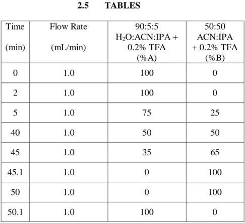
Table 2.1. Chromatographic conditions for the reversed-phase prefractionation of

intact proteins. ... 52 Table 2.2. Integrated TIC values, summed integrated TIC, and normalized

summed integrated TIC value used to determine first dimension

fractionation schemes. ... 53 Table 2.3. The protein coverage (%) was reported for some of the proteins

involved in S. cerevisiae metabolism. Generally, protein coverage

increased with fractionation frequency. ... 55 Table 2.4. The Grand NDPC and Fold-Change in Coverage was listed in for each

fractionation frequency. Positive values represented higher coverage with the equal-mass fractionation method, and negative values represented higher coverage with the equal-time fractionation method. The Grand NDPC and Fold-Change in Coverage favored of the equal-mass method for 5 and 10. The largest fold-change improvement was 1.4 with the 10 fraction comparison. No significant difference in coverage was observed

between the two methods with 20 first dimension fractions. ... 56 Table 3.1. The methods as programmed into MassLynx were listed along with the

valve timings. The gradient loading time was listed as x, where x equals the gradient volume divided by the flow rate when loading the gradient.

The time to play back the gradient was listed as y. ... 101 Table 3.2. The dimensions for each of the analytical columns tested in this

manuscript were listed along with their measured flow rates and

programmed gradient volumes. ... 102 Table 3.3. The number of theoretical plates was calculated for several gradient

storage loop internal diameters and gradient volumes. ... 103 Table 3.4. The retention times, in minutes, were listed for several peptides

identified in an enolase digest standatd separated on a 110 cm x 75 µm column packed with 1.9 µm BEH C18 particles. The gradient volume was 12.5 µL and was repeated 12 times on 12 different days. The retentions

times all had an %RSD of 4.5% or less. ... 104 Table 3.5. The average separation window, peak width (4σ), peak capacity, and

number of protein and peptide identifications were listed for each column

at each running condition. ... 105 Table 3.6. The Grand NDPC and Fold-Change Coverage were compared for E.

(15)

represented higher coverage on the shorter column. Grand NDPC and Fold-Change Coverage increased in favor of the long column as gradient

length increased. ... 106 Table 4.1. To assess the stability of peptides at elevated pressures and

temperatures, the MassPrep standard protein digest was storage for 10

hours at the conditions listed in this table. ... 149 Table 4.2. To assess the stability of peptides at elevated temperatures for 2-10

hours, the enolase digest standard was storage at the conditions marked by

an “X” on this table. ... 150

Table 4.3. The number of significantly different peak intensities are listed for the enolase digest sample stored in 4% mobile phase B at 25, 35, 45, 55, and 65°C for 2, 4, 6, 8, and 10 hours. Intensities were compared to the unstressed, control sample A in which 19 peptide peaks were identified. Most of the identified peptide peaks do not have significantly different intensities when stored at any temperature for 6 hours. After 8 and 10 hours, many more peptides have significantly different intensities. At these extreme conditions, about 6-7 peaks, or 35% of all identifications,

have significantly different intensities. ... 151 Table 4.4. The number of significantly different peak intensities are listed for the

enolase digest sample stored in 40% mobile phase B at 25, 35, 45, 55, and 65°C for 2, 4, 6, 8, and 10 hours. Intensities were compared to the

unstressed, control sample B in which 13 peptide peaks were identified. Most of the identified peptide peaks do not have significantly different intensities when stored at any temperature for 6 hours. After 8 hours at 65°C, a couple more peptides have significantly different intensities. At this extreme condition, two to three peaks, or 19% of all identifications,

had significantly different intensities. ... 152 Table 4.5. The retention times and mass-to-charge ratios (m/z) are listed for peaks

that appeared after the enolase digest was stored in the indicated sample solution. The 199.1 m/z peak appeared when the enolase digest standard was stored in 4% mobile phase B for extended periods of time above 45°C. This peak is not observed when the sample was stored in 40% mobile phase B. The other two peaks were degradation products extracted

from the polypropylene microcentrifuge tubes used for sample storage. ... 153 Table 5.1. Chromatographic conditions for the reversed-phase prefractionation of

intact proteins. ... 182 Table 5.2. The fractionation schemes for a set of 20 (a), 10 (b), and 5 (c) first

dimension fractions are listed with the associated first dimension

(16)

Table 5.3. The method for the second dimension separation at ultrahigh pressure

as programmed into MassLynx is listed along with the valve timings. ... 184 Table 5.4. For the separations on the modified UHPLC, the protein coverage (%)

and number of peptides used to identify each protein is reported for the

some of the proteins involved in S. cerevisiae metabolism ... 185 Table 5.5. The Grand NDPC and Fold-Change in Coverage are listed for each

fractionation frequency. Positive values represent higher coverage when the 110cm long column at 32 kpsi was used for the second dimension separation as compared to the shorter column run on the standard system. The Fold-Change in Coverage increased as fractionation frequency

decreased. ... 186 Table 6.1. Chromatographic conditions for the reversed-phase prefractionation of

intact proteins. ... 224 Table 6.2. The first dimension prefractionation times of yeast grown on dextrose

and glycerol are listed with the associated normalized Σ absorbance. ... 225

Table 6.3. The method for the second dimension separation at ultrahigh pressure,

as programmed into MassLynx, is listed along with the valve timings. ... 226 Table 6.4. The protein coverage (%) and number of peptides used to identify each

protein are reported for the some of the proteins involved in S. cerevisiae

metabolism. ... 227 Table 6.5. The Grand NDPC and Fold-Change in Coverage are listed for each

fractionation frequency. The positive values represent higher coverage with the 5 equal-mass fractions run on the 110 cm long column at 32 kpsi as described in this chapter. A negative value would have indicated higher coverage by our previous results from the 20 equal-time fraction run on the 25 cm commercial column at 8 kpsi on the standard UPLC.21 The improvement is small but impressive when one considers that the total

separation time was reduced four fold. ... 228 Table 6.6. The T-test confidence value, p-value, fold change, and average

quantitative value was reported for the some of the proteins involved in S. cerevisiae metabolism. The quantative value was determined as the

(17)

LIST OF FIGURES

Figure 1.1. The explanation for the flow of genetic information through the biological system is referred to as the central dogma. DNA is transcribed into RNA which is translated into proteins. The proteins regulate

metabolites which result in the observed phenotype. ... 16 Figure 1.2. A small portion of the regulatory pathways involved in S. cerevisiae

metabolism is shown. Proteins in red were up-regulated in yeast grown on glycerol, and proteins in blue were up-regulated in yeast grown on

dextrose. Small molecules involved in the pathway are in italics. For this differential study, it is evident that glycerol catabolism, TCA, glyoxylate cycles are more active for metabolizing glycerol while fermentation and

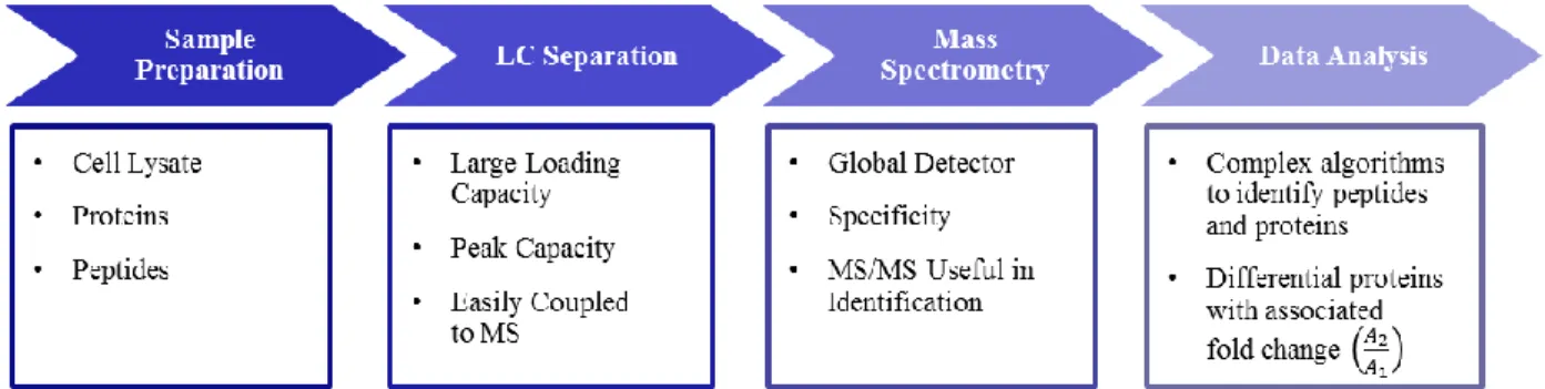
glycerolneogenesis occurs in dextrose metabolism.26 ... 17 Figure 1.3. A workflow is outlined for a generic proteomics experiment. The

experiment starts with a cell lysate. The analyte is either proteins or peptides. The sample is separated, commonly by liquid chromatography (LC), because it has a large loading capacity and peak capacity. LC is easily coupled to a mass spectrometer. Through electrospray, the ionization of peptides and proteins is possible making MS a near global detector. Specificity of MS, based on mass-to-charge, adds another level of separation. The fragmentation data associated from MS/MS

experiments is useful in identifying the protein. Complex algorithms process the spectral data to identify peptides and proteins. The relative abundance, usually in terms of spectral counts, is calculated to give the fold change in expression of a protein in two differential proteomic

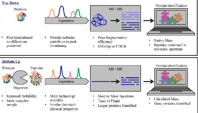
samples... 18 Figure 1.4. Typical work flows for top-down and bottom-up experiments with

considerations for each step are shown. ... 19 Figure 1.5. Example spectra of protein envelops acquired by ESI-TOF-MS are

shown drawn to the same intensity scale. Myoglobin and bovine serum albumin (BSA) were infused in similar amounts. Bovine serum albumin (a) is 66 kDa and much larger than 17 kDa myoglobin (b). The BSA molecules are split over more charge states than myoglobin making it less

intense and more difficult to detect. ... 20 Figure 1.6. This diagram shows two adjacent peaks, with retention times tr,1 and

tr,1 and peak widths of 4σ at 11% of the maximum height. The two peaks

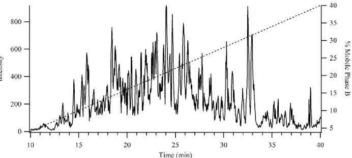
have a resolution of 1. ... 21 Figure 1.7. This example separation is of a standard enolase protein digest. This

separation has a peak capacity of 100 which is typical for a 30 minute gradient on a standard UPLC with a commercial column. A peak capacity

(18)

Figure 1.8. An example separation (nc=100) of an E. coli digest shows many

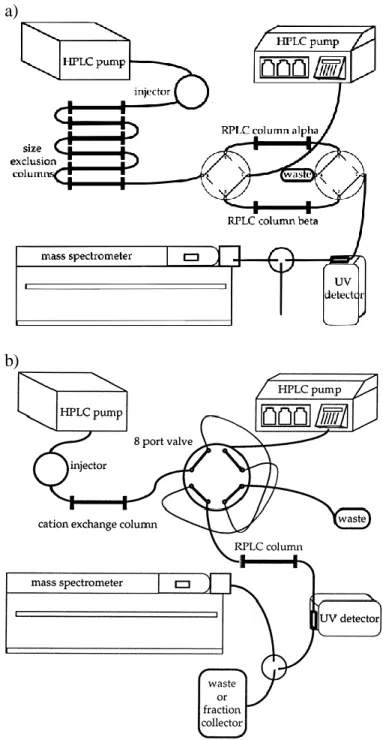
overlapping peaks. ... 23 Figure 1.9. Two instrument schematics are shown for an online multidimensional

separation. In part (a), there are two identical columns (A and B) in the second dimension. The effluent from the first separation is loaded onto the head of column A. Using two 4-port valves, the effluent is then switched to column B, and a gradient is pumped through column A to complete the second-dimension separation. This cycle continues until the desired number of fractions from the first dimension is obtained.84 Alternatively, this can be completed with one second-dimension column using two

storage loops between the dimensions as shown in part (b).80,85 ... 24 Figure 1.10. The top-down 2D chromatogram shows S. cerevisiae separated on a

strong anion-exchange column in the first dimension and reversed-phase

column in the second dimension.88 ... 25 Figure 1.11. The 2D chromatogram shows the bottom-up separation of S.

cerevisiae. A step gradient is implemented for the first dimension separation. There were five steps dictating the peak capacity of the first dimension. A reversed-phase column is used in both dimensions. The separation attempts to be orthogonal by modifying the sample with high-pH mobile phase in the first dimension and low-high-pH mobile phase in the

second dimension.88 ... 26 Figure 2.1. This 2D chromatogram was divided in to bins by Davis and

coworkers.7 A perimeter was drawn around the bins containing a circle, which represented a sample peak, to illustrate the orthogonality of the

separation. ... 57 Figure 2.2. The workflow for the prefractionation method started with HPLC-UV

of the intact proteins. Forty fractions were collected, lyophilized, and digested with trypsin. The forty one-minute-wide fractions were pooled into 20, 10, and 5 equal-time and equal-mass fractions before the second dimension analysis by UPLC-MS. The spectral data was searched against

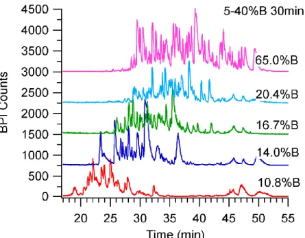
a genomic database to identify the proteins. ... 58 Figure 2.3. The representative TIC chromatogram from a peptide (second

dimension) separation of the 40 equal-time fraction set showed an example of peak integration. The peak area was the ∫TIC value used in Table 2.2 for the determination of the equal-mass prefractionation

schemes. ... 59 Figure 2.4. (a) The normalized Σ∫TIC, Σ absorbance, and summed unique protein

(19)

parts (b), (c), and (d), respectively. Lines were drawn from the hash marks on the y-axis to the corresponding x-coordinate on the normalized equal-mass curve. These x-coordinates were used to determine size of the first

dimension fractions... 60 Figure 2.5. The number of protein identifications was plotted versus number of

first dimension fractions. The blue and red traces were for the equal-time and equal-mass fractionation methods, respectively. The number of protein identifications increased with increased prefractionation up to 40 fractions. At all prefractionation frequencies, the equal-mass

prefractionation method outperformed the equal-time prefractionation

method. ... 61 Figure 2.6. The 2D chromatogram for 40 first dimension fractions was plotted

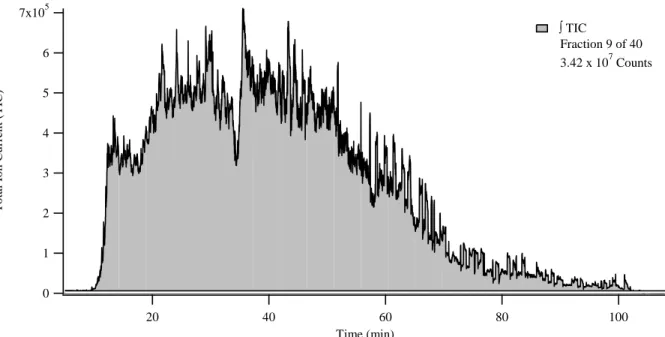
with the first dimension (protein) separation time and fraction number plotted on the vertical axes and the second dimension (peptide) separation on the bottom axis. Starting with fraction 30, the peak pattern repeated for all subsequent fractions. These peaks corresponded to peptides from

trypsin autolysis. ... 62 Figure 2.7. The 2D chromatograms for 20 first dimension fractions were plotted

with the first dimension (protein) separation time or fraction number plotted on the vertical axes and the second dimension (peptide) separation on the bottom axis. Peak intensity was plotted in the z-direction. In the later eluting fractions, more peaks were observed in (b) the equal-mass fractionation chromatogram than in (a) the equal-time fractionation

chromatogram... 63 Figure 2.8. The 2D chromatograms for 10 first dimension fractions were plotted

chromatogram... 64 Figure 2.9. The 2D chromatograms for 5 first dimension fractions were plotted

chromatogram... 65 Figure 2.10. The light gray bars show the total protein identifications in each

(20)

protein identifications decreased in the last 15 fractions faster than the total protein identifications. This trend was less pronounced as

prefractionation frequency decreased. a) ... 66 Figure 2.11. The light gray bars show the total protein identifications in each

fraction, and the dark gray bars signify the unique protein identifications in each fraction for 20 first dimensional fractions. By more evenly

distributing the sample mass between the fractions, as with the equal-mass fractionation method (b), the number of unique protein identifications was more even fraction to fraction and increased in the late eluting fractions as

compared to the equal-time fractionation method (a).a) ... 67 Figure 2.12. The light gray bars show the total protein identifications in each

compared to the equal-time fractionation method (a). ... 68 Figure 2.13. The light gray bars show the total protein identifications in each

compared to the equal-time fractionation method (a). ... 69 Figure 2.14. Venn diagram (a) showed the overlap in protein identifications for 5,

10, and 20 equal-time fractions. Increasing fractionation to 20 led to new protein identifications while still identifying most of the proteins identified in the five and ten fraction sets. Venn diagram (b) showed the overlap in

protein identifications for 20 and 40 equal-time fractions. ... 70 Figure 2.15. The Venn diagram showed the overlap in protein identifications for

5, 10, and 20 equal-mass fractions. Increasing fractionation to 20 led to new protein identifications while still identifying most of the proteins

identified in the five and ten fraction sets. ... 71 Figure 2.16. Fractions per protein described the percentage of protein

identifications that were detected in one, two, or more fractions (3+). As prefractionation frequency increased, more proteins were identified in multiple fractions. This effect was heightened for the equal-time fractions

(blue) as compared to the equal-mass fractions (red). ... 72 Figure 2.17. To compare the 5 equal-mass and 5 equal-time fractions, the

(21)

proteins with higher coverage on the left, and proteins with lower coverage on the right. If a protein was identified with higher sequence coverage in the 5 equal-mass fractions, its NDPC value was positive (red bars). The blue bars signified higher coverage in the 5 equal-time

fractions. Differences in coverage were minimal for highly covered proteins. As protein coverage decreased, more proteins were identified with higher coverage in the equal-mass fractions. The dashed lines

indicate a level of two-fold greater protein coverage. ... 73 Figure 2.18. The NDPC compared the equal-mass and equal-time methods for 5

(part a), 10 (part b), and 20 (part c) first dimension fractions. If a protein was identified with higher sequence coverage in the equal-mass fractions, the NDPC value was positive (red lines). The blue lines signified higher coverage in the equal-time fractions. Proteins with higher coverage were plotted on the left, and proteins with lower coverage were on the right. Differences in coverage were minimal for highly covered proteins. As protein coverage decreased, more proteins were identified with higher coverage by the equal-mass method for 5 and 10 fractions. There was little

difference in NDPC for 20 equal-mass and 20 equal-time fractions. ... 76 Figure 3.1. The nanoAcquity was shown with the additional tubing and valves

necessary for separations at 45 kpsi driven by the Haskel pneumatic

amplifier pump. ... 107 Figure 3.2. The gradient playback time of the UHPLC was monitored by the UV

absorbance of acetone in mobile phase B. The gradient linearity was improved by using a lower flow rate for gradient loading and employing

the 50 µL ID tubing at the head of the gradient storage loop. ... 108 Figure 3.3. The gradient playback time of the UHPLC was monitored by the UV

absorbance of acetone in mobile phase B and plotted in part (a) for several different gradient volumes which were noted on the graph. The playback time of the linear region was plotted versus gradient volume in part (b). A best fit line had the equation y = 3.33x – 4.19 and R2 value of 0.999. The

inverse slope was 0.300 µL/min which corresponded to flow rate. ... 109 Figure 3.4. The retention time residuals were plotted versus run order for several

peptides identified in an enolase digest standard separated on a 110 cm x 75 µm column packed with 1.9 µm BEH C18 particles. The gradient volume was 12.5 µL and was repeated 12 times on 12 different days. The variability of retention times was random with the R2 values for a 5th order

polynomial fit of the residuals ranging between 0.57 and 0.69. ... 110 Figure 3.5. The Van Deemter plots with reduced terms of hydroquinone

demonstrate the similarity in column performance for the columns tested

(22)

Figure 3.6. Chromatograms of MassPREPTM Digestion Standard Protein Expression Mixture 2 were collected for separations with increasing gradient volume on the 44.1 cm x 75 µm ID column packed with 1.9 µm BEH C18 particles. Separations were completed at 15 kpsi. The insert of a representative peptide peak with 724 m/z extracted from all four

chromatograms demonstrated the increase in peak width and decrease in

peak height as the as gradient volume increased. ... 112 Figure 3.7. Chromatograms of MassPREPTM Digestion Standard Protein

Expression Mixture 2 were collected for separations with increasing pressure and flow rate on the 44.1 cm x 75 µm ID column packed with 1.9 µm BEH C18 particles. Separations were completed with a 56 µL gradient volume. The insert of a representative peptide peak with 724 m/z extracted from all three chromatograms showed the decrease in peak width and

constant signal intensity as pressure and flow rate increased. ... 113 Figure 3.8. Peak capacity versus separation window was displayed for separations

on a 44.1 cm x 75 µm ID column with 1.9 µm BEH C18 particles. Each line represented a different running pressure, and each point on a line (from left to right) represented the gradient profiles of 4, 2, 1, or 0.5

percent change in mobile phase composition per column volume. ... 114 Figure 3.9. Chromatograms of MassPREPTME. coli Digestion Standard were

collected for separations with increasing gradient volume on the 44.1 cm x 75 µm ID column packed with 1.9 µm BEH C18 particles. Separations were completed at 15 kpsi. Though the chromatograms were very busy, an increase in resolution was observed as gradient volume increased which was indicated by the signal being closer to baseline between two adjacent

peaks. ... 115 Figure 3.10. Chromatograms of MassPREPTME. coli Digestion Standard were

collected for separations with increasing pressure and flow rate on the 44.1 cm x 75 µm ID column packed with 1.9 µm BEH C18 particles.

Separations were completed with a 56 µL gradient volume. ... 116 Figure 3.11. The peptide and protein identifications for E. coli were plotted versus

the separation window and peak capacity for several separations on a 44.1 cm x 75 µm ID column with 1.9 µm BEH C18 particles. Each line

represents a different running pressure, and each point on a line (from left to right) represented the gradient profiles of 4, 2, 1, or 0.5 percent change

in mobile phase per column volume. ... 117 Figure 3.12. Protein identifications per minute or productivity was plotted for the

E. coli protein identifications from analyses at varying gradient volumes and pressures on the 44.1 cm x 75 µm ID column with 1.9 µm BEH C18 particles. Productivity was highest for the steepest gradient run at the

(23)

Figure 3.13. Chromatograms of MassPREPTM Digestion Standard Protein Expression Mixture 2 were collected for separations with increasing pressure on a short and long column. The separation time was similar for the 98.2 cm x 75 µm ID column and 44.1 cm x 75 µm ID column packed with 1.9 µm BEH C18 particles. The insert of a representative peptide peak with 724 m/z extracted from both chromatograms showed the decrease in peak width and constant signal intensity as pressure and

column length increased. ... 119 Figure 3.14. The increasing peak capacity versus separation window plot

demonstrated the benefit of using higher pressures to run longer columns in the same amount of time as shorter columns. The red line represented separations at 15 kpsi on a 44.1 cm x 75 µm ID column with 1.9 µm BEH C18 particles. The blue line represented separations at 30 kpsi on a 98.2 cm x 75 µm ID column with 1.9 µm BEH C18 particles. The gray line represented separations on a commercial UPLC with a commercial

column (25 cm x 75 µm ID column with 1.9 µm BEH C18 particles). Each point on a line (from left to right) represented the gradient profiles of 4, 2,

1, or 0.5 percent change in mobile phase per column volume. ... 120 Figure 3.15. Chromatograms of MassPREPTME. coli Digestion Standard were

collected for separations with increasing gradient volume on the 98.2 cm x 75 µm ID column packed with 1.9 µm BEH C18 particles. Separations were completed at 30 kpsi. Though the chromatograms were very busy, an increase in resolution was observed as gradient volume increased which was indicated by the signal being closer to baseline between two adjacent peaks. These were the shotgun proteomic experiments with the highest

peak capacities. ... 121 Figure 3.16. This chromatogram of MassPREPTME. coli Digestion Standard from

the 98.2 cm x 75 µm ID column packed with 1.9 µm BEH C18 particles is a zoomed in version of the purple chromatogram in Figure 3.15. The return of signal to baseline between several adjacent peaks demonstrated the gain in resolution from using long columns at elevated pressures and

temperature for proteomics analysis. ... 122 Figure 3.17. The peptide and protein identifications for E. coli were plotted versus

the separation window in parts a and b, respectively. The red line

represented separations at 15 kpsi on a 44.1 cm x 75 µm ID column with 1.9 µm BEH C18 particles. The blue line represented separations at 30 kpsi on a 98.2 cm x 75 µm ID column with 1.9 µm BEH C18 particles. The gray line represented separations on a commercial UPLC with a commercial column (25 cm x 75 µm ID column with 1.9 µm BEH 18 particles). Each point on a line (from left to right) represented the gradient profiles of 4, 2, 1, or 0.5 percent change in mobile phase per column

(24)

Figure 3.18. The NDPC comparing the analysis on the 98.2 cm column run at 30 kpsi to the 44.1 cm column run at 15 kpsi for a 360 min gradient was plotted for each protein identified in an E. coli digest standard. If a protein was identified with higher sequence coverage with the separation on the 98.2 cm column, its NDPC value was positive (blue bars). The red bars signified higher coverage with the separation on the 44.1 cm column. Proteins with higher coverage were plotted on the left, and proteins with lower coverage were on the right. Differences in coverage were minimal for highly covered proteins. As protein coverage decreased, more proteins were identified with higher coverage with the separation on the 98.2 cm column. The dashed line represented a two-fold difference in protein

coverage. ... 124 Figure 3.19. The NDPC comparing the analysis on the 98.2 cm column run at 30

kpsi to the 44.1 cm column run at 15 kpsi was plotted for each protein identified in an E. coli digest standard separated with a for a 90 min (part a), 180 min (part b), and 360 min (part c) gradient . If a protein was identified with higher sequence coverage with the separation on the 98.2 cm column, its NDPC value was positive (blue bars). The red bars signified higher coverage with the separation on the 44.1 cm column. Proteins with higher coverage were plotted on the left, and proteins with lower coverage were on the right. Differences in coverage were minimal for highly covered proteins. As protein coverage decreased, more proteins were identified with higher coverage with the separation on the 98.2 cm

column. ... 127 Figure 3.20. Chromatograms of MassPREPTM Digestion Standard Protein

Expression Mixture 2 were collected for separations with increasing gradient volume on the 39.2 cm x 75 µm ID column packed with 1.4 µm BEH C18 particles. Separations were completed at 30 kpsi. The insert of a representative peptide peak with 724 m/z extracted from all four

chromatograms showed the increase in peak width and decrease in peak

height as the as gradient volume increased. ... 128 Figure 3.21. Chromatograms of MassPREPTM Digestion Standard Protein

Expression Mixture 2 were collected for separations with increasing gradient volume on the 28.5 cm x 75 µm ID column packed with 1.1 µm BEH C18 particles. Separations were completed at 30 kpsi. The insert of a representative peptide peak with 724 m/z extracted from all four

chromatograms showed the increase in peak width and decrease in peak height as the as gradient volume increased. These were the fasted

separations demonstrated in this manuscript. The gain in speed was due to

the implementation of small particles and ultrahigh pressures. ... 129 Figure 3.22. The increasing peak capacity versus separation window plot

(25)

x 75 µm ID column with 1.4 µm BEH C18 particles. The blue line represented separations on a 98.2 cm x 75 µm ID column with 1.9 µm BEH C18 particles. The green line represented separations on a 28.5 cm x 75 µm ID column with 1.1 µm BEH C18 particles. The gray line

represented separations on a commercial UPLC with a commercial

column. ... 130 Figure 3.23. The peak capacity versus separation window plot compared the

highest peak capacities demonstrated in this manuscript, as obtained with the 98.2 cm x 75 µm ID column with 1.9 µm BEH C18 particles,

separations on the commercial nanoAcquity and several data sets found in the literature for separations with long columns and at high pressure (PNNL24,Harvard39). The data presented in this manuscript achieved

higher peak capacities in less time as compared to the literature data. ... 131 Figure 4.1. The instrument diagram (a) shows the fluidic configuration for sample

storage at elevated pressures and temperatures. Part (b) shows the fluidic configuration for gradient/sample loading and sample analysis. For gradient/sample loading, all valves were opened except the nanoAcquity vent valve. For sample storage and analysis, all valves were closed except the nanoAcquity vent valve. The haskel pump and column heater were regulated to the desired pressure and temperature to stress the sample. During analysis, the haskel pump and column heater were regulated to 15

kpsi and 30°C. ... 154 Figure 4.2. These chromatograms were from the analysis of the standard protein

digest stored in the gradient storage loop. Storage conditions are listed

above each chromatogram. ... 155 Figure 4.3. These Venn diagrams show the similarities in peptide identification

for the standard protein digest control sample compared to a replicate

analysis and to analysis of the sample stored at stress conditions... 156 Figure 4.4. The log peptide intensities are plotted comparing two replicate

analyses of the control standard protein digest. The confidence lines drawn on the graph are used to describe the scatter from the dashed y=x line due to analytical variability. The formulas for each line and the percent of data

points contained within each set of lines are listed in the legend. ... 157 Figure 4.5. The log peptide intensities are plotted for the standard protein digest

stored at 45 kpsi and ambient temperature for 10 hours compared to the control. As listed in the legend, 95.2% of the data points are contained within the green lines. This percentage is greater than that expected due to analytical variability which indicates no change in peptide intensity from

(26)

Figure 4.6. The log peptide intensities are plotted for the standard protein digest stored at 65°C and ambient pressure for 10 hours compared to the control. As listed in the legend, 91.5% of the data points are contained within the green lines. This percentage is less than that expected due to analytical variability. Most of the variability occurs from data points falling below the y=x dashed line which indicates a decrease of intensity for peptides in

the elevated temperature sample. ... 159 Figure 4.7. The log peptide intensities are plotted for the standard protein digest

stored at 65°C and 45 kpsi for 10 hours compared to the control. As listed in the legend, 88.8% of the data points are contained within the green lines. This percentage is less than that expected due to analytical

variability. Most of the variability occurs from data points falling below the y=x dashed line which indicates a decrease of intensity for peptides in

the stressed sample. ... 160 Figure 4.8. These red and blue chromatograms are from the analysis of the

enolase digest control and stress sample stored at 65°C for 10 hours. Feature A (199.1 m/z) is a degradation peak that appeared when enolase was stored in 4% mobile phase B at elevated temperatures. The green chromatogram of mobile phase stored in the polypropylene

microcentrifuge tubes at 65°C for 10 hours shows that peak B (460.4 m/z) and peak C (780.9 m/z) were extracted from the tube and are not peptide

degradation products. ... 161 Figure 4.9. The intensity is plotted versus storage time for a degradation peak

(199.1 m/z) that appeared when the enolase digest standard was stored in 4% mobile phase B for extended periods of time. This peak appeared when the sample was stored above 45°C. This peak is not observed when

the sample was stored in 40% mobile phase B. ... 162 Figure 5.1. The workflow for the prefractionation method started with HPLC-UV

of the intact proteins. Thirty-eight one-minute-wide fractions were collected, lyophilized, and pooled into 20 equal-mass fractions. The 20 mass fractions were digested and also pooled into 10 and 5 equal-mass fractions. The set of 20, 10, and 5 equal-equal-mass fractions were

analyzed with a second dimension separation by the modified UHPLC-MS at 32 kpsi. The spectral data were searched against a genomic database to

identify the proteins. ... 187 Figure 5.2. The normalized ΣAbsorbance trace is plotted versus the first

dimension separation time to determine the equal-mass prefractionation timings. The y-axis is equally divided into 20 (a), 10 (b), and 5 (c) fractions. A line is drawn from the Σ Absorbance trace to the x-axis to determine when to take fractions from the first dimension. The UV chromatogram is overlaid on these plots to show how the area under the

(27)

Figure 5.3. The number of protein identifications is plotted versus number of first dimension fractions. The green line is for the prefractionation experiment, described in this chapter, run on the modified UHPLC at 32 kpsi. As a comparison, the results from this chapter where superimposed on Figure 2.5 (red and blue traces) for a prefractionation study with a standard UPLC. The number of protein identifications greatly increased through

use of long columns on the UHPLC. ... 189 Figure 5.4. Two-dimensional chromatograms for 20 (a,b), 10 (c,d), and 5 (e,f)

first dimension fractions are plotted with the first dimension (protein) fraction number versus the second dimension (peptide) separation. Base peak intensity BPI is plotted in the z-direction. Chromatograms on the left (a,c,e) are from the modified UHPLCat 32 kpsi with a 110 cm column, and chromatograms on the right (b,d,f) are run on a standard UPLC at 8 kpsi with a 25 cm commercial column. The same amount of protein was loaded onto the column in both analyses. The gain in intensity was due to

the decreased peak widths on the longer column. ... 190 Figure 5.5. On average, more unique proteins were identified per fraction as

prefractionation frequency decreased but total proteins identifications per fraction remained constant. The light gray bars show the total protein identifications in each fraction, and the dark gray bars signify the unique protein identifications in each fraction for 20 (a), 10 (b), and 5 (c) first dimensional fractions analyzed on the modified UHPLC at 32 kpsi. The x-axis is the first dimension separation time with the UV absorbance

overlaid in red... 191 Figure 5.6. More proteins were identified per fraction when the fractions were run

on the 110 cm column at 32 kpsi (a) as compared to the standard UPLC (b). The light gray bars show the total protein identifications in each fraction, and the dark gray bars signify the unique protein identifications

in each fraction for 20 first dimension fractions. ... 192 Figure 5.7. More proteins were identified per fraction when the fractions were run

on the 110 cm column at 32 kpsi (a) as compared to the standard UPLC (b).The light gray bars show the total protein identifications in each fraction, and the dark gray bars signify the unique protein identifications

in each fraction for 10 first dimension fractions. ... 193 Figure 5.8. More proteins were identified per fraction when the fractions were run

on the 110 cm column at 32 kpsi (a) as compared to the standard UPLC (b).The light gray bars show the total protein identifications in each fraction, and the dark gray bars signify the unique protein identifications

in each fraction for 5 first dimension fractions. ... 194 Figure 5.9. These histograms display the protein molecular weight distributions

(28)

mass distribution corresponding to the 5, 10 and 20 fractions are portrayed by the black, gray and white bars, respectively. Proteins were identified with masses up to 250 kDa. For all methods, the median molecular weight was 39-40 kDa. For the fractions run at 32 kpsi, the increase in

identifications occurred mostly for lower mass proteins 20-70 kDa. ... 195 Figure 5.10. The mass chromatograms for 20 (a,b), 10 (c,d), and 5 (e,f) first

dimension fractions are plotted as protein mass versus first dimension fraction. The log quantitative value for each protein is plotted in the z-direction. Chromatograms on the left (a,c,e) are from the modified UHPLC at 32 kpsi on a 110 cm column, and chromatograms on the right (b,d,f) are from the standard UPLC at 8 kpsi on a 25 cm commercial

column. ... 196 Figure 5.11. Similarities in protein identifications are compared for 5 (a), 10 (b),

and 20 (c) first dimension fractions run on the 110 cm column at 32 kpsi

to fractions run on a standard UPLC. ... 197 Figure 5.12. The Venn diagram demonstrates the overlap in protein identifications

for 5, 10, and 20 equal-mass fractions run on the 110 cm column at 32

kpsi... 198 Figure 5.13. Fractions per protein describe the percentage of proteins that were

identified in one, two or more (3+) fractions run on the 110 cm column at 32 kpsi (a) and the standard UPLC (b). As prefractionation frequency increased, more proteins were identified in multiple fractions. A larger percentage of the proteins were identified in multiple fractions with the modified system. The increased identification of proteins across multiple fractions was mostly likely related to the increased peak intensities in the

second dimension separation... 199 Figure 5.14. To compare the 5 fractions run on the modified system to the 5

fractions run on the standard UPLC, the NDPC is plotted with proteins with higher coverage on the left, and proteins with lower coverage on the right. If a protein was identified with higher sequence coverage when analyzed on the modified UHPLC, its NDPC value is positive (blue bars). The red bars signify higher coverage in the analysis on the standard UPLC. Differences in coverage were minimal for highly covered proteins. As protein coverage decreased, more proteins were identified with higher coverage from the analysis on the modified UHPLC. The dashed lines indicate a level of two-fold greater protein coverage. (This was a large

graph and split into multiple parts.) ... 200 Figure 5.15. The NDPC plotted here compare proteins identified with the

(29)

lines). The red lines signify higher coverage with the standard UPLC. Proteins with higher coverage are plotted on the left, and proteins with lower coverage are on the right. More proteins were identified with higher

coverage by with the modified UHPLC. ... 205 Figure 6.1. The workflow for the prefractionation method started with HPLC-UV

of the intact proteins. Thirty-eight one-minute-wide fractions were

collected, lyophilized, and pooled into 20 mass fractions. The equal-mass fractions were digested and pooled into 5 equal-equal-mass fractions before the second dimension analysis by the modified UHPLC-MS at 32 kpsi. The spectral data was searched against a genomic database to

identify the proteins. ... 230 Figure 6.2. The normalized Σ absorbance, plotted here with the UV

chromatograms, was used to distribute the first dimension separation for

yeast grown on dextrose (a) and glycerol (b) into equal-mass fractions. ... 231 Figure 6.3. Two-dimensional chromatograms for yeast grown on dextrose (a) and

glycerol (b) are plotted with the first dimension (protein) fraction number on the vertical axes and the second dimension (peptide) separation on the

bottom axes. Peak intensity (BPI) is plotted in the z-direction. ... 232 Figure 6.4. The light gray bars show the total protein identifications in each

fraction, and the dark gray bars signify the unique protein identifications in each fraction for yeast grown on dextrose (a) and glycerol (b) with the

UV chromatogram of the first dimension separation overlaid. ... 233 Figure 6.5. Fractions per protein describe the percentage of protein identifications

that were detected in one, two, three, four, or all five fractions. ... 234 Figure 6.6. The overlap in identifications is shown for yeast grown on dextrose

and glycerol. ... 235 Figure 6.7. The –log10 (p-value) is plotted versus the log2 fold change (a). All

points above the horizontal dashed line represent significantly different protein quantities with 95% minimum confidence. A negative or positive fold change is a convention for up-regulation of the protein in yeast grown on dextrose or glycerol, respectively. All points outside the vertical dashed lines represent a fold change greater that two. Protein quantity is not captured in the volcano plot so the log of the quantitative value for all significantly different proteins is plotted (b). Proteins up-regulated in the dextrose or glycerol sample are closer to the y-axis or x-axis, respectively. Points falling along the axis were only identified in the sample

corresponding to that axis. The solid line represents y=x, and the dashed

(30)

fermentation, TCA cycle, and glyoxylate cycle are depicted with protein identifiers in blue or red if the protein was up-regulated when yeast was grown on the dextrose or glycerol media, respectively. Identifiers in black represent proteins that were identified without a significant difference in abundance. They gray text shows what metabolite are involved in the

(31)

LIST OF APPENDED FIGURES

Appendix A.1. To compare the 10 equal-mass and 10 equal-time fractions, the Normalized Difference Protein Coverage (NDPC) was plotted with proteins with higher coverage on the left, and proteins with lower coverage on the right. If a protein was identified with higher sequence coverage in the 10 equal-mass fractions, its NDPC value was positive (red bars). The blue bars signified higher coverage in the 10 equal-time

fractions. Differences in coverage were minimal for highly covered proteins. As protein coverage decreased, more proteins were identified with higher coverage in the equal-mass fractions. The dashed lines

indicate a level of two-fold greater protein coverage. ... 243 Appendix A.2. To compare the 20 equal-mass and 20 equal-time fractions, the

Normalized Difference Protein Coverage (NDPC) was plotted with proteins with higher coverage on the left, and proteins with lower coverage on the right. If a protein was identified with higher sequence coverage in the 20 equal-mass fractions, its NDPC value was positive (red bars). The blue bars signified higher coverage in the 20 equal-time

fractions. Differences in coverage were minimal for highly covered proteins. For 20 fractions, the NDPC did not favor the equal-mass or the equal-time fractionation methods. The dashed lines indicate a level of

two-fold greater protein coverage. ... 246 Appendix B.1. The NDPC comparing the analysis on the 98.2 cm column run at

30 kpsi to the 44.1 cm column run at 15 kpsi for a 90 min gradient was plotted for each protein identified in an E. coli digest standard. If a protein was identified with higher sequence coverage with the separation on the 98.2 cm column, its NDPC value was positive (blue bars). The red bars signified higher coverage with the separation on the 44.1 cm column. Proteins with higher coverage were plotted on the left, and proteins with lower coverage were on the right. Differences in coverage were minimal for highly covered proteins. As protein coverage decreased, more proteins were identified with higher coverage with the separation on the 98.2 cm column. The dashed line represented a two-fold difference in protein

coverage. ... 251 Appendix B.2. The NDPC comparing the analysis on the 98.2 cm column run at

(32)

column. The dashed line represented a two-fold difference in protein

coverage. ... 254 Appendix B.3. Chromatograms of MassPREPTM Digestion Standard Protein

Expression Mixture 2 were collected for separations with increasing pressure and flow rate on the 39.2 cm x 75 µm ID column packed with 1.4 µm BEH C18 particles. Separations were completed with a 50µL gradient volume. The insert of a representative peptide peak with 724 m/z extracted from all three chromatograms showed the decrease in peak width and

constant signal intensity as pressure and flow rate increased. ... 257 Appendix B.4. Chromatograms of MassPREPTME. coli Digestion Standard were

collected for separations with increasing gradient volume on the 39.2 cm x 75 µm ID column packed with 1.4 µm BEH C18 particles. Separations were completed at 30 kpsi. Though the chromatograms were very busy, an increase in resolution was observed as gradient volume increased which was indicated by the signal being closer to baseline between two adjacent

peaks. ... 258 Appendix B.5. Chromatograms of MassPREPTME. coli Digestion Standard were

collected for separations with increasing pressure and flow rate on the 39.2 cm x 75 µm ID column packed with 1.4 µm BEH C18 particles.

Separations were completed with a 50µL gradient volume. ... 259 Appendix C.1. To compare the 10 fractions run on the modified system to the 10

graph and split into multiple parts.) ... 260 Appendix C.2. To compare the 20 fractions run on the modified system to the 20

(33)

LIST OF ABBREVIATIONS AND SYMBOLS

%A percent mobile phase A

%B percent mobile phase B

∫TIC integrated total ion current

°C degrees Celsius

2D two dimensional

2DLC two-dimensional liquid chromatography

2D-PAGE two-dimensional polyacrylamide gel electrophoresis

A absorbance

Å angstrom

ACN acetonitrile

ACS American chemical society

BEH bridged ethyl hybrid

BPI base peak intensity

BSA bovine serum albumin

cm centimeter

dc column diameter

Dm diffusion in the mobile phase

ESI electrospray ionization

F flow rate

FTICR Fourier transform ion cyclotron resonance

g gram

(34)

Hcm height equivalent of a theoretical plate

(resistance to mass transfer in the mobile phase)

ID internal diameter

IDs identifications

IEX ion-exchange chromatography

IPA 2-propanol

iTRAQ isobaric-tag-for-relative-and-absolute-quantification

kDa kiloDalton

kpsi kilo pounds per square inch

kV kilovolts

L liter

L length

LC liquid chromatography

LIFO last in first out

M molar

m meter

m/z mass to charge ratio

MALDI matrix assisted laser desorption ionization

mg milligram

min minute

mL milliliter

mM millimolar

mm millimeter

(35)

MS mass spectrometry

MSE mass spectrometry expression

N number of theoretical plates

nc peak capacity

NDPC normalized difference protein coverage

ng nanogram

nL nanoliter

nm nanometer

np practical peak capacity

O.D. optical density

pI isoelectric point

PLGS ProteinLynx Global Server

PLRP-S polystyrene-divinylbenzene reversed-phase HPLC column

Pmax maximum peak capacity

pmol picomole

PPP pentose phosphate pathway

psi pounds per square inch

qTOF quadrapole time-of-flight

Rep replicate

RPLC reversed-phase liquid chromatography SEC size exclusion chromatography

sec second

(36)

SILAC stable-isotope-labeling-by-amino-acids-in-cell-culture

t time

TCA the citric acid cycle

TCPK tosyl phenylalanyl chloromethyl ketone, chymotrypsin inhibitor

td dead time

TFA trifluoroacetic acid

tg gradient time

TIC total ion current

tm mobile phase time

u linear velocity

UHPLC ultrahigh pressure liquid chromatography UPLC ultrahigh performance liquid chromatography

UV ultraviolet

V volts

V volume

v/v volume per volume

v:v:v volume to volume to volume ratio

Vis visible

w/w weight per weight

Xg times gravity

YAPG yeast agar peptone glycerol

μg microgram

(37)

μm micrometer

Σ∫TIC summed integrated total ion current

(38)

CHAPTER 1. An Introduction to Differential Proteomics by Multidimensional Liquid Chromatography-Mass Spectrometry

1.1 Introduction

Protein regulation has long been studied to better understand biological processes.1 Analyses of proteins are complicated because there are thousands of proteins in a cell spanning a

large range of abundances (upwards of 1010).2 A common approach to study protein regulation is by differential proteomics using multidimensional chromatography to separate the complex mixture followed by detection with mass spectrometry (MS).3,4 In this introductory chapter, the

need for studying differential protein regulation by multidimensional chromatography-MS will be explained.5 Several accomplishments made in this field will be reviewed. Building on the

ideas discussed in this introduction, the aim of this dissertation will be to improve the coverage of a model proteome, Saccharomyces cerevisiae, through the development of separation methods and instrumentation.

1.2 Why study proteomics?

For many years, scientists have been trying to understand why certain phenotypes are

observed in nature.6,7,8 For example, why do certain populations of people develop diabetes or heart disease while others do not? Some causes are environmental, such as diet and exercise, but

other causes are inherently biological.9,10 The central dogma (Figure 1.1) is described as the flow of genetic information through the biological system.11 As the central dogma progresses from DNA, to RNA, to proteins, and finally metabolites, the complexity increases in both number of

(39)

20 endogenous amino acids,11 and metabolites can be a variety of small molecules including carbohydrates, lipids, etc.14 As complexity of the biological sample increases, the burden on the

analytical method to study these molecules also increases.15,16,17

Scientists believed that unlocking the genomic code would demystify the existence of

certain phenotypes.18 In the 1990s, the United States government funded the completion of the human genome.19,20 However, scientists soon learned that not all of the genome is transcribed into RNA,21 and not all RNA is translated into proteins. Proteins control cellular pathways, and

the metabolites, involved in these pathways actually, account for the phenotype. After

translation, the protein can be further modified with functional groups such as acetate, phosphate,

lipids and carbohydrates. These post-translational modifications (PTMs) extend the function of the protein.11 For the regulatory role that proteins play in biological pathways, the field of proteomics emerged.22, 23,24

1.2.1 Differential proteomics

Consider two cell types, with different genetic variants or observed phenotypes.

Determining which proteins are up and down regulated between the two samples can shed light onto what biological pathways are active. This study of relative protein abundance became

known as differential proteomics.5,25 For example, Figure 1.2. shows a portion of the regulatory pathways involved in S. cerevisiae (yeast) metabolism.26 Proteins in red were up-regulated in yeast grown on glycerol, and proteins in blue were up-regulated in yeast grown on dextrose.

From this differential study, it is evident that the citric acid (TCA) and glyoxylate cycles are more active when metabolizing glycerol, and fermentation is preferred for dextrose metabolism.

(40)

range of expression levels.27 To tackle these experimental challenges, a need arises to have better resolution, a large dynamic range and global yet specific detection.28

1.2.2 Differential proteomic tools

Many tools and methods have been developed to study differential proteomics.28 This

chapter aims to highlight some common practices and fundamentally ground breaking techniques. A generic workflow is outlined in Figure 1.3. The experiment starts with a cell lysate. The analyte either contains intact proteins or peptides from the digested proteins. The

sample is separated, commonly by liquid chromatography (LC), because it has a large loading capacity and high resolution.4 Loading capacity is necessary because analysis of a large amount

of total protein may be required to detect a single analyte of low abundance. LC is also easily coupled to a mass spectrometer. Through electrospray, the ionization of peptides and proteins is possible making MS the near global detector for proteomics. Specificity of the MS, based on

mass-to-charge, adds another level of separation.4 The fragmentation data, from MS/MS

experiments, are useful in identifying the protein.29,30 The spectral data is compared to a genomic

database, using complex computer algorithms, to identify peptides and proteins.31,32 The relative abundance, usually in terms of a ratio of spectral counts, is calculated to give the fold change in

expression of a protein in two differential proteomic samples.33

To help with the quantitative analysis of mass spectral data, several common strategies can be executed such as isobaric-tag-for-relative-and-absolute-quantification (iTRAQ),

stable-isotope-labeling-by-amino-acids-in-cell-culture (SILAC), and label-free.25,34 iTRAQ allows for absolute quantification by adding an isobaric label to the N-terminus and amine side chains of

(41)

enriched medium for the other sample. Commonly, arginine labeled with 12C and 13C atoms are used for the normal and enriched media, respectively.37,38 Both iTRAQ and SILAC label the

sample, which greatly reduces analysis time, because differential samples can be pooled prior to the separation. The spectral data for each sample is deconvoluted by the mass shift due to the

label. Analyzing both samples simultaneously reduces the day-to-day variability that can occur from temperature changes in the laboratory. The major advantages of label-free relative

quantification are lower cost and a reduced risk of modifying the sample in the labeling process.

Also, the spectra are not busy with isobaric and isotopic data. The validity of quantification based on spectral counts with the label-free method has been demonstrated in the literature.39,40,41

1.3 Choice of strategy: top-down versus bottom-up 1.3.1 Sample preparation and separation

The first step in analyzing proteomics samples is to decide between a top-down (protein)

or bottom-up (peptide) strategy.30 Typical work flows with considerations for each step are shown in Figure 1.4. The top-down experiment begins with the separation of intact proteins. A

single protein may exist in many different isoforms and have different post-translational modifications which would contribute to band broadening.42 Maintaining the solubility of

proteins outside of the cell is difficult.43 Low solubility has limited the development of new technology for the separation of intact proteins.44 For this reason, many scientists prefer to do a bottom-up experiment in which the proteins are enzymatically digested, into peptides prior to

analysis.39 Trypsin, the most commonly used digest enzyme, cleaves proteins on the C-terminal side of arginine and lysine residues creating peptides about 20 amino acids in length.45 Proteins

(42)

1.3.2 Mass spectral detection

After the separation, the analytes are introduced into the mass spectrometer. Mass

spectrometry of large biological molecules remained elusive until the invention of matrix

assisted laser desorption ionization (MALDI) and electrospray ionization (ESI). For MALDI, the

matrix is ablated with a laser initiating desorption and ionization of the analyte. The resulting spectrum, obtained with a time-of-flight (TOF) mass analyzer, contains predominantly singly

charged ions with large peak widths contributing to low resolution (R=m

m, typically 300-400 for proteins).47,48 ESI has become the preferred source due to its easy coupling with LC where a high voltage electric field is applied to a narrow capillary. The liquid becomes a fine aerosol, and ions

are completely desolvated before entering the MS.49 The spectrum, from an ESI-TOF-MS, contains multiply charged ions and has a higher resolution than MALDI (R=50000).50 With the ability to analyze peptides and proteins by MS, the sample components don’t have to be

completely separated by LC because the MS can detect many species in a single scan. Furthermore, the development of gas phase ion mobility adds the option of a post-ionization

separation without adding to the total analysis time.51 However, ionization suppression and matrix effects still plague mass spectrometric techniques, necessitating separation prior to analysis.52,53

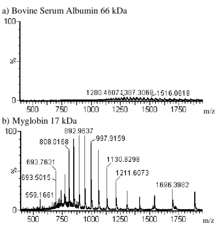
The ESI spectral data from top-down experiments are complex due to the many charge states of intact proteins.54 Example spectra, drawn on the same intensity scale, are shown in