Environmental Research and Public Health
Article
A Multivariate Dynamic Spatial Factor Model for
Speciated Pollutants and Adverse Birth Outcomes
Kimberly A. Kaufeld1,∗, Montse Fuentes2, Brian J. Reich3, Amy H. Herring4, Gary M. Shaw5 and Maria A. Terres6
1 Los Alamos National Laboratory, P.O. Box 1663, Los Alamos, NM 87545, USA
2 Department of Biostatistics and Statistics and Operations Research, Virginia Commonwealth University,
Richmond, VA 23284, USA; [email protected]
3 Department of Statistics, North Carolina State University, Raleigh, NC 27695, USA; [email protected]
4 Department of Biostatistics, University of North Carolina, Chapel Hill, NC 27599, USA; [email protected]
5 Division of Neonatology, Department of Pediatrics, Stanford University School of Medicine, Stanford,
CA 94305, USA; [email protected]
6 The Climate Corporation, San Francisco, CA 94103, USA; [email protected]
* Correspondence: [email protected]
Received: 31 May 2017; Accepted: 1 September 2017; Published: 11 September 2017
Abstract: Evidence suggests that exposure to elevated concentrations of air pollution during pregnancy is associated with increased risks of birth defects and other adverse birth outcomes. While current regulations put limits on total PM2.5concentrations, there are many speciated pollutants within this size class that likely have distinct effects on perinatal health. However, due to correlations between these speciated pollutants, it can be difficult to decipher their effects in a model for birth outcomes. To combat this difficulty, we develop a multivariate spatio-temporal Bayesian model for speciated particulate matter using dynamic spatial factors. These spatial factors can then be interpolated to the pregnant women’s homes to be used to model birth defects. The birth defect model allows the impact of pollutants to vary across different weeks of the pregnancy in order to identify susceptible periods. The proposed methodology is illustrated using pollutant monitoring data from the Environmental Protection Agency and birth records from the National Birth Defect Prevention Study.
Keywords:multivariate; spatiotemporal; birth defects; pollutants; factor analysis
1. Introduction
The association of air pollution exposure and adverse pregnancy outcomes has been found in a number of recent studies. Zeiger and Beaty [1] mention that both genetic and environmental factors play important roles in oral clefts. In a fetal study on rats, exposure to ozone and carbon monoxide produced a skeletal malformation in animals [2,3]. Air pollution was also found to contribute to the development of skeletal malformations via toxicity and biologic mechanisms [4].
Several studies have found adverse effects of air pollution exposure during pregnancy and birth defects [4,5]. In a case control study of women in Los Angeles, Ritz et al. [4] found an association of air pollution, CO and ozone, O3, exposure and birth defects including oral clefts. In another study, the amount of exposure to O3during the first and second month of pregnancy was found to increase the risk of oral clefts [6], one of the types of orofacial clefts. In one study conducted in China, environmental factors were found to be more strongly associated with cleft lip and/or palate [7]. In another study in Texas, there was a weak association between particulate matter, PM10, and isolated cleft lip with or without cleft palate [5]. A study conducted in the California National Birth Defects
Prevention Study (NBDPS) region, Padula et al. [8] found associations between traffic density and cleft lip with or without palate, but no associations with particulate matter and birth defects.
A common statistical challenge in these epidemiological studies is estimating a mother’s exposure with sparse monitor locations [9]. Studies have recommended including only mothers within 6 km or 12 km of a monitoring station [10]. However, in many birth defect studies, the mother is often assigned to the nearest air pollution monitor [4,5,11]. As there are approximately 40 stations in all of California, the distance to a monitor and quality of the proxy can vary dramatically depending upon where a woman resides. In our study, we interpolate the factors of the pollutants using a geospatial approach, Gaussian processes, at the mother’s location rather than only to the closest location. This allows us to get a more accurate idea of the the impact of the factors at different times of the mothers’ pregnancy and can help account for the maternal proximity to high areas of pollution.
In our study, we investigate the effects of speciated components, the particles that compose particulate matter, PM2.5, to help determine which components have a more significant impact on cleft birth defects. Earlier studies only used O3and total PM2.5[4,11]. We extend the results to account for several pollutants during critical gestation periods when women are more susceptible to pollutants. Exposure is usually aggregated to the month or trimester, and only a few studies have looked at exposure at the weekly level in association with selected birth defects [12–14]. In the weekly model, a Bayesian hierarchical framework was developed to assess critical windows of exposure between weeks 3–8. It used weekly averages during embryonic development and identified windows using a non-Gaussian and spatial-temporal associations. The model, however, did not look at multiple pollutants simultaneously.
Our model expands upon spatial dynamic factor analysis recently proposed in the literature by including a multivariate dimension of factors while simultaneously modeling the health effects. The spatial dynamic factor analysis developed by Lopes et al. [15] differs in two key ways. First, their approach is presented for univariate spatio-temporal data, whereas ours allows for consideration of multiple spatio-temporal processes (pollutants) jointly. Secondly, the factors in their model are purely temporal and thus only allow for examination of spatial variation in the factor loadings, not in the factors themselves. In contrast, the Bayesian spatial confirmatory factor analysis for climate is illustrated by Neeley et al. [16] is both multivariate and produces a spatial factor. In particular, the spatial factor represents a weighted average of the original multivariate spatial processes with spatially smooth factor loadings. However, this analysis was developed for areal data using a conditionally autoregressive (CAR) structure and does not capture temporal evolution in the processes. Our proposed model merges ideas from each of these papers in order to produce a multivariate spatial dynamic factor model with spatio-temporal factors that evolve coherently in time, while simultaneously relates the factor to the health outcomes.
In our model, the spatio-temporal factors are utilized as predictors in a model for human health (e.g., risk of birth defect). The work of Jandarov and Szpiro [17] has a similar goal, but utilizes principal components (PC) in lieu of a factor model. The PC scores vary spatially and are regressed on geographical covariates with a Gaussian process error allowing for interpolation at new locations. The framework does not, however, incorporate any temporal structure into the model. In contrast, our approach is fit in a Bayesian framework and produces interpretable spatial factor loadings and temporal dynamics. In this paper, we introduce a spatial dynamic factor model using Bayesian multivariate (binary) probit regression. The model accounts for multiple pollutants in the factor component model at the critical times in a mother’s pregnancy, weeks 3–8.
Network (STN) and Interagency Monitoring for Protected Visual Environments (IMPROVE) that provide ambient monitoring station data.
In Section2, we describe the data used in the analysis. Section3introduces the statistical model. In Section4, the spatial dynamic factor model is applied to the California birth defects dataset including a short sensitivity analysis of the factors. In Section5, we close with conclusions and discussions.
2. Data Description
2.1. National Birth Defects Data
The oral cleft defects data in California is from the National Birth Defects Prevention Study, a population-based, multi-center case control study of birth defects [18]. It includes information on live births from 2002 to 2008 in California. The methods are described in Reefhuis et al. [18]. Cases included live births, and controls are live births without any known birth defects, identified randomly from selected hospitals in California. We analyzed both cleft lip and cleft palate defects. There were a total of 208 cleft lip or cleft palate defects reported and 358 controls. Cases listed as cleft palate include a cleft lip and cleft palate defect, similarly cleft lip includes a cleft lip and cleft palate defect.
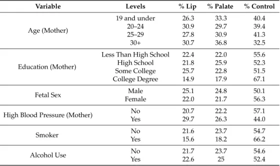
As part of the study, women reported their complete residential history during pregnancy. Based upon this information, all residences were geocoded at the first eight weeks of pregnancy to assign exposure levels. The NBDPS protocol estimates each woman’s date of conception based upon the estimated date of delivery—in other words, the due date that the woman received from her physician, which was reported at the study interview. The estimated date of conception is used to identify exposure levels during gestation periods, weeks 3–8, the pertinent embryologic period of lip and palate formation. In the case that a woman had more than one residence, the mother was assigned a different exposure level based upon the residing location. We also used potential confounder variables displayed in Table1: sex of the infant, maternal education (high school, some college and college), maternal age classifications (19 and under, 20–24, 25–29, 30–34, and 35 and older), high blood pressure during pregnancy, smoking while pregnant and alcohol use while pregnant.
Table 1.Cleft defect variables tabulated by maternal and fetal characteristics, cleft lip includes both cleft lip and cleft lip and palate defects; similarly, cleft palate includes both cleft palate and cleft lip and cleft palate defects.
Variable Levels % Lip % Palate % Control
Age (Mother)
19 and under 26.3 33.3 40.4
20–24 30.9 29.7 39.4
25–29 27.8 30.9 41.3
30+ 30.7 36.8 32.5
Education (Mother)
Less Than High School 22.4 22.0 55.6
High School 21.8 25.9 52.3
Some College 25.7 22.8 51.5
College Degree 14.9 17.9 67.1
Fetal Sex Male 25.1 24.8 50.1
Female 22.0 21.7 56.3
High Blood Pressure (Mother) No 20.7 22.2 57.1
Yes 29.7 26.3 44.0
Smoker No 21.6 23.7 54.7
Yes 15.6 18.2 66.2
Alcohol Use No 21.7 23.7 54.6
2.2. Pollution Data
The AQS monitoring data collected by the Environmental Protection Agency (EPA) are available for California from 2003 to 2007. Speciated PM2.5values in micrograms per cubic meter (ug/m3) are collected to construct a map of the pollutant sites in the state of California. Although the birth defects study does not cover all of California, we use all the station data to help account for a mother’s mobility during the study period. There were approximately 15% of the women moved during the study to areas outside of the initial study area. In some cases, areas moved to are not in the original study area, thus it is important to include stations from outside the study region in this case including all stations in California. These data consist of measurements collected every three to six days by the EPA’s Interagency Monitoring for Protected Visual Environments (IMPROVE) and STN sites. The IMPROVE monitors are located in more remote areas, while the STN monitors are located in more urban areas. The two monitoring networks have 40 monitors, and 20 are in the study region, combining the two data sources provides good coverage of California. The speciated components selected for the study are Ammonium, Nitrate, Sulfate, Total Carbon, Calcium, Iron, Potassium, Silicon, and Sulfur.
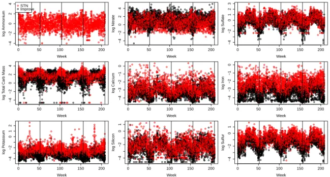
The speciated components are combined by a dynamic spatial factor analysis, and resulting factors are interpolated using bivariate spline interpolation, a geospatial technique, to each mother in the study. The interpolated factors represent the ambient concentration at the mother’s residence. The weekly factor averages for gestational weeks three through eight are considered based on embryonic timing of an association with orofacial clefts. The nine speciated components, at each site, are averaged weekly from 2003 to 2006. All sites pollutant values are shown on the log scale in Figure1. A clear seasonal pattern can be found across the speciated pollutants, which is captured in the dynamic model.
0 50 100 150 200
−4 −2 0 2 4 Week log Ammonium STN Improve
0 50 100 150 200
−4 −2 0 2 4 Week log Nitr ate
0 50 100 150 200
−4 −2 0 1 2 3 Week log Sulf ate
0 50 100 150 200
−4 −2 0 2 4 Week log T
otal Carb Mass
0 50 100 150 200
−4 −3 −2 −1 0 Week log Calcium
0 50 100 150 200
−4 −3 −2 −1 0 Week log Iron
0 50 100 150 200
−4 −2 0 1 2 Week log P otassium
0 50 100 150 200
−4 −2 0 1 Week log Silicon
0 50 100 150 200
−4 −2 0 1 Week log Sulfur
Figure 1.STN and IMPROVE stations speciated components for the years 2003–2006 weekly averages for each site where the vertical lines separate each year. Ammonium is only collected at STN sites.
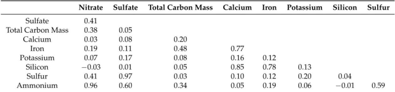
Table 2.Pearson correlation coefficients of weekly speciated pollutants from stations relevant to the study in the state of California, 2003–2006.
Nitrate Sulfate Total Carbon Mass Calcium Iron Potassium Silicon Sulfur
Sulfate 0.41
Total Carbon Mass 0.38 0.05
Calcium 0.03 0.08 0.20
Iron 0.19 0.11 0.48 0.77
Potassium 0.07 0.17 0.08 0.16 0.12
Silicon −0.03 0.01 0.05 0.85 0.78 0.13
Sulfur 0.41 0.97 0.03 0.10 0.12 0.20 0.04
Ammonium 0.96 0.60 0.34 0.05 0.19 0.06 −0.01 0.59
3. Multivariate Spatio-Temporal Factor Model for Pollution
In this section, we describe our model to relate the speciated particulate matter mixture with birth defect outcomes. Our model expands upon spatial dynamic factor analysis recently proposed in the literature by including a multivariate dimension of factors while simultaneously modeling the health effects. In Section 3.1, we give the spatiotemporal factor model for speciated PM2.5. In Section3.2, we give the model to relate the latent particulate matter factors with the health outcomes. Although the aspects of the model are described separately, they are fit simultaneously using a Bayesian hierarchical model, the pollutant model is evaluated at the first stage and the birth defect model is estimated at the second stage in one algorithm. The computational algorithm with the priors for the model is described in the Appendix.
3.1. Factor Model for Speciated PM2.5
The factor model for speciated PM2.5 expands upon the spatial dynamic factor analysis presented for univariate spatio-temporal data, recently proposed in the literature by Lopes et al. [15]. The extension of the proposed model allows for consideration of multiple spatio-temporal processes (pollutants) jointly as well as providing spatial variation in the factors. We use the notation similar to Lopes et al. [15] as follows.
LetYtp(s) be the observation at location s on day t = 1, . . . ,T, for pollutant p = 1, . . . ,P,
andYt(s) = [Yt1(s), . . . ,YtP(s)]T. The high correlations between pollutants, as shown in Section2.2,
and spatial variability in the pollutant sources favors dimension reduction in the number of pollutants. We useM≤Platent factors to represent variation in thePpollutants. Letδt(s) = [δt1(s), . . . ,δtM(s)]T
be the latent vector of factors for timetat locations.
Our model is a dynamic linear model with observation and evolution equations:
Yt(s) =µt(s) +Λ(s)δt(s) +et(s), (1)
δt(s) =Γ(s)δt−1(s) +wt(s).
In Equation (1), µt(s) = [µt1(s), . . . ,µtP(s)]T is the P-vector of means that vary slowly over
time to capture seasonality (e.g., Figure1); Λ(s) is the P×M factor loading matrix that relates the latent factors to the observed pollutant concentrations;Γ(s)is theM×Mmatrix that controls the propagation of the latent factors; et(s) = [et1(s), . . . ,etP(s)]T are errors withetj(s) ∼ N(0,σ2);
andwt(s) = [wt1(s), . . . ,wtM(s)]Tcaptures the spatial process at locationsusing a zero mean Gaussian
process with varianceV[wtl(s)] = s2w and spatial correlation cor[wtl(s),wtl(s0)] = R(||s−s0||j,φw)
denotedwtl ∼GP[0,s2wR(φw)].
The effect of factorf on pollutantpis determined by the(p,f)element ofΛ(s), denoted byλp f(s).
To ensure identification, we fixλp f(s) =0 for f <pandλp f(s)>0 forp=1, . . . ,M. To induce spatial
smoothness in the loadings, we model the elements log[λpp(s)]andλp f(s)for f > pas realizations
from a Gaussian process,GP[0,s2λ
The propagation matrixΓ(s)is taken to be diagonal with diagonal elements γ1(s), . . . ,γM(s)
for identification in the case where factors are rotated. Spatial smoothness in the evolution processes
γp(s)is again desirable, so we model them as a Gaussian process,γf ∼GP[0,s2ΓfR(φΓf)]. We constrain
the factor evolution coefficients, γf, to the interval (−1, 1)to ensure stationarity of the temporal
processes using a truncated Gaussian process [19]. Finally, to ensure spatial smoothness in the dynamic factors, the initial valuesδ0are each assumed to be a realization from a Gaussian process, δf,0∼GP[0,s2δfR(φδf)]. We have assumed that theµvector will center the pollutant quantities such
that the means of the factors, factor loadings, and factor evolution coefficients will be 0.
In summary, an observationYtp(s)of pollutantpat locationsand timetwill be centered atµtp(s)
plus some linear function of the Mfactors at locationsand timet. These factors will be spatially smooth and evolve in time therefore accounting for the underlying correlation structure. The mutual dependence on the sameMfactors builds dependence between thePpollutants. Imagine we have
M=2 sources of pollution, say traffic and factories. We have no direct measures of these sources,δt1(s) andδt2(s), so we instead relate these latent factors to speciated pollution levels, say organic carbon, elemental carbon, nitrate and sulfate, whichcanbe measured. At any location, the measured pollutant level will depend on the pollutant sources as determined byΛ(s). Through the use of spatially varying factor loadings, the current model allows, for example, the amount of nitrate in traffic pollution to vary spatially. In one area, the factor loading may be high, indicating that the traffic pollution is particularly high in nitrate, while, in another area, it may be low indicating that traffic pollution is relatively low in nitrate. In the case of spatially constant factor loadings, the model would suggest that traffic produces a fixed amount of nitrate relative to its abundance regardless of location.
3.2. Tailoring the Pollutant Model to CA Pollutant Data
The general spatial dynamic factor model described in Section3.1is augmented to fit the ambient air pollutant data in California described in Section2. The pollutant data are from two observation networks: STN for urban sites and IMPROVE (IMP) for rural sites. We allow the mean and error variances to differ based upon the pollutants sites in the model by accounting for the two networks in Equation (1) as follows:
µtp(s) =
( ¯
µ0pifsis an IMPROVE site,
¯
µ0p+µ¯1pifsis a STN site,
andet,p(s)∼N[0,σ2p(s)], where
σtp2 =
σSTN2 ,p
σI MP2 ,p.
The speciated components, accounting for the two observation networks, are combined via the dynamic spatial factor analysis described in Section3.1. The model reduces the speciated components to only a few factors. The resulting factors from the model are then interpolated to the mother’s location based upon the prior distributions (see Appendix A) of the factors. The weekly factors associated with each woman during gestational weeks 3 through 8, corresponding to the embryonic timing for cleft defects, are consequently used in the birth defect model as described below.
3.3. Birth Defect Model
The California birth defect data has two binary responses denoted
˜
Yi1=
(
0, no cleft palate defect,
˜
Yi2=
(
0, no cleft lip defect,
1, cleft lip defect for individuali.
The multiple binary responses are modeled using probit regression to induce conjugacy to simultaneously fit the factor and birth defect models in the Bayesian hierarchical setting. The probability of having a cleft defect is modeled assuming a set of latent variables,Zi = (Zi1,Zi2) such that ˜Yij=I(Zij>0)and
Zi =βTxi+ M
∑
m=1
L=8
∑
`=3wT`mδi`m+ei.
The vectorxicontains individual-level covariates such as maternal age (Table1),βis a matrix of regression coefficients specific to the birth defect which relates the covariates, i.e., fetus’ gender, mother’s age, race, etc., to the latent response,wT`mrepresents the effect of exposure to factormduring gestation week`,δi`mis the value of factormfor motheriat gestation week`, i.e., a specific value of
the latent factors,δtj(s), from Equation (1) andei~N(0,Ω). The latent variables,Zi, are used to define
the outcomes when ˜Yij=1, i.e., defectjwas observed ifZij >0, whereas if a control was observed,
Zij < 0. This lends itself to interpretation of the probability of a defect, P(Zij > 0), or if a control
is observed P(Zij < 0). Therefore, the probability of ˜Yij = 1, P( ˜Yij = 1) is equal toΦ(βTxi+wδi),
whereΦis the standard normal distribution function that increases with the linear predictorβTxi+wδi.
For example, if one element ofβis positive, then an increase in the corresponding covariate increases the probability of a defect. On the other hand, if one element ofβis negative, then a decrease in the corresponding covariate decreases the probability of a defect.
To account for the effects of pollutants at different gestation times of the pregnancy, the temporal covariates from theMfactors are accounted for using a Gaussian process
wTm ∼GP[0,R(φ)],
where the coefficients are allowed to change smoothly across pregnancy weeks. In this case,wmT are the coefficients for each of theZiclefts (cleft lip and cleft palate) weekly measurements of pollutant indexM(factors). For example, if one element ofwis positive, then an increase in the corresponding pollutant factor increases the probability of a defect and vice versa.
As this is a fully Bayesian approach, the model is specified by assigning prior distributions to the model parameters. The mean coefficients areβ∼N(0, I). In this model, cleft lip and cleft palate can occur at the same time, and are not mutually exclusive. The correlation coefficient between defects isφ =0.51. To account for the correlation structure, we use an inverse Wishart for the covariance structure,Ω∼ IW(Σ,ν), whereΣ= I2andν=2.
The self reported confounders inxiinclude indicators for maternal age categories 19 and under, 20–24, 25–29, 30 and older; maternal education categorized as less than high school, high school diploma/equivalency and/or some college or trade school and college graduate or advanced degree; binary indicators of maternal smoking during pregnancy categorized as yes/no; maternal alcohol consumption during the pregnancy as any/none; maternal prediabetes, high blood pressure; and sex of the fetus.
4. Results
4.1. Impacts on Oral Cleft Risks
20,000 draws from the posterior distribution after a burn-in period of 5000 draws. These values were determined by trace plots for stability in the chains.
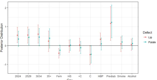
Table3and Figure2display the posterior summaries for the effect of the covariates. For example, if one of the coefficients is positive, it increases the probability of a defect, whereas a negative coefficient decreases the probability of a defect. The age of the mother increases the the probability of cleft defects, both lip and palate. There is a general trend that any age group over 19 has a higher risk of defects compared to the baseline group of ages 19 and under, with cleft lip defects having a slightly higher probability for ages 20–34. The age group 35 and over also has an increased probability of defects; however, it is not significant for either cleft lip or cleft palate defect. Another covariate that increases the probability either a cleft lip or cleft palate defect is mothers with prediabetes. There is also an increase in the probability of a cleft palate defect if the mother has high blood pressure. However, it was not found to be a significant factor for cleft palate. The covariates that portray a decrease in the probability of a defect include the mother having a college education compared to less than a high school education for both cleft lip and cleft palate. If the sex of the fetus is female, the probability of a cleft lip defect is lower compared to a male fetus. Interestingly, smoking and alcohol use did not contribute significantly to cleft lip or cleft palate defect, which may be partially due to mothers in the study self reporting substance use.
Table 3.The posterior means, standard deviation (SD), and quantiles for a change in cleft lip defects (top) and cleft palate defects (bottom) in the National Birth Defects Prevention Study, 2003–2007.
Mean SD 2.5% 50% 97.5%
Maternal age 20–24 vs. 19 and under 0.540 0.208 0.150 0.545 0.958
Maternal age 25–29 vs. 19 and under 0.556 0.222 0.128 0.562 0.976
Maternal age 30–24 vs. 19 and under 0.605 0.245 0.127 0.609 1.094
Maternal age 35+ vs. 19 and under 0.232 0.285 −0.310 0.217 0.764
Fetus Sex-Female −0.405 0.134 −0.664 −0.407 −0.157
High school diploma vs. Less than high school −0.021 0.164 −0.354 −0.019 0.290 Some college vs. Less than high school 0.032 0.173 −0.296 0.027 0.388 College graduate vs. Less than high school −0.480 0.258 −1.003 −0.469 −0.009
High Blood Pressure 0.332 0.165 0.017 0.330 0.671
Maternal Prediabetes 1.175 0.449 0.261 1.181 2.070
Maternal Smoking 0.089 0.192 −0.310 0.091 0.454
Maternal Alcohol Use 0.049 0.149 −0.243 0.052 0.348
Maternal age 20–24 vs. 19 and under 0.345 0.198 −0.048 0.345 0.760
Maternal age 25–29 vs. 19 and under 0.439 0.208 0.027 0.437 0.866
Maternal age 30–34 vs. 19 and under 0.440 0.231 −0.018 0.428 0.899
Maternal age 35+ vs. 19 and under 0.385 0.268 −0.139 0.381 0.895
Fetus Sex-Female −0.247 0.133 −0.503 −0.246 0.021
High School Education vs. Less than high school 0.023 0.150 −0.262 0.026 0.309 Some college vs. Less than high school −0.109 0.169 −0.426 −0.114 0.209 College graduate vs. Less than high school −0.430 0.167 −0.943 −0.412 −0.001
High Blood Pressure 0.05 0.155 −0.221 0.007 0.332
Maternal Prediabetes 1.214 0.431 0.391 1.196 2.072
Maternal Smoking 0.183 0.174 −0.153 0.190 0.510
Figure 2.Covariate effects for the multivariate binary probit model. The posterior means (dots) and 95% credible intervals (lines) for a change in cleft defects with a one-standard deviation increase in maternal age, education, maternal smoking, and maternal alcohol consumption in the California National Birth Defects Prevention Study, 2003–2006. The labels from left to right are maternal age 20–24 vs. 19 and under (2024), 25–29 vs. 19 and under (2529), 30–34 vs. 19 and under (3034), 35+ vs. 19 and under (35+), fetus sex-female (Fem), maternal high school education vs. less than high school (HS), some college vs. less than high school (<C), college graduate vs. less than high school (C), high blood pressure (HBP), maternal prediabetes (Prediab), maternal smoking (Smoke), maternal alcohol (Alcohol).
4.2. Model Comparison
We compare M = 1,2, and 3 factor models using the deviance information criterion (DIC) of Spiegelhalter et al. [20]. DIC is based upon the posterior distribution of the deviance statistic, D(θ) =−2 log(p(Y˜|θ)),wherep(Y˜|θ)represents the likelihood of the observed data given the vector of all model parameters,θ. The posterior expectation of the deviance,D¯,describes the fit of the model to the data andpD=D¯−D(θ)¯ describes the complexity of the model based upon an effective number of parameters. DIC is defined as DIC =D¯ +pD, the lower the value of DIC the better the fit.
Comparison of the models show that DIC is lowest for the one-factor model (DIC = 1624.06) compared to the two-factor (DIC = 1628.15) and three-factor (DIC = 1629.98) models. Although there was not a large difference in DIC for the three models, the impact of pollutants each week are more clearly defined in the one-factor model and therefore we proceed with theM =1to present the results. To further see how the model fits, we checked the predicted probabilities for the one factor model to see how well the model classified the defects. The percent of defects that were correctly identified as defects,P(Yˆ =1|Y =1), came to approximately 92%, resulting in only 8% of the defects classified incorrectly.
4.3. Latent Factor Results
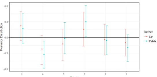
Figure 3.Weekly association of latent pollutants factors (w`m) for the one-factor model. The effects
are summarized by their posterior means (dots) and 95% credible intervals (vertical lines) for a change in cleft defects with a one-standard deviation increase in the mixture of pollutant exposure during weeks 3 through 8 post-conception in the National Birth Defects Prevention Study, 2003–2007. The factor pollutants are adjusted for maternal age, education, maternal smoking, and maternal alcohol use. Weeks 4, 5, 7 and 8 are associated with a slightly lower probability of having a cleft palate defect, whereas exposure during weeks 3 and 6 is associated with a slight increase in the probability of having a cleft palate defect.
To gain a better understanding of the impact the individual pollutants have on clefts for the one factor model, the estimated pollutants and the average of all the factor components,δ(s), are compared. We note that, although the study region was conducted in central California, we present estimates for the entire state to help account for the mother’s movement during the study. Approximately 15% of the women moved during the duration of the study to areas outside of the initial study area, with the majority of the women moving to the San Francisco Bay area, Los Angeles and the San Diego area. These are high density population areas that generally have high concentrations of pollutants. To gain a more complete understanding of the individual pollutant effects, we standardized the estimated pollutants in CA. The daily mean standardized estimated pollutants,(Yp−µYp)/σYp is
displayed in Figure4. In the main study area, Central Valley of California, the highest concentrations of speciated pollutants are identified as Calcium, Total Carbon Mass, Sulfate and Potassium. Total carbon mass has a more equal concentration of pollutant values across the state of California. In high density areas, such as Los Angeles and San Diego, there is a general pattern of higher concentrations of Ammonium, Nitrate, Sulfate, and Sulfur. If the mother moved during the study period to any of these areas, the fetus would likely have been exposed to higher concentrations of pollutants. In the southeast corner of the state near the Nevada border, near Las Vegas on the Nevada side, higher concentrations of Total Carbon, Potassium, Iron, Sulfate and Ammonium are present, although not as high as the Bay area and Los Angeles. The factor components (δ’s) show a higher concentration of pollutants in the mid to southeastern side of California, part of the study region, and the coastal area near San Francisco.
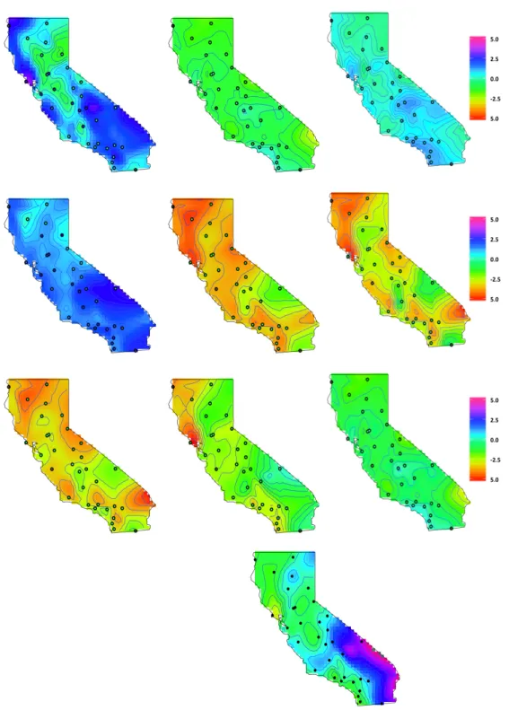
Figure 5.California factor loadings. TheΛp(s)are (1st row) Ammonium, Nitrate, Sulfate, (2nd row)
Total Carbon Mass, Calcium, Iron and (3rd row) Potassium, Silicon, and Sulfur. The dots represent the STN and IMPROVE monitoring sites.
San Franscisco area and Los Angeles, which are high pollutant areas. In general, other pollutants such as Iron and Calcium did not contribute much to the latent factor model.
5. Conclusions
We constructed a spatiotemporal model that accounts for different sources of speciated pollutants and their association with oral cleft birth defects. Our factor model has advantages over other pollutant models because it accounts for the bias in monitoring stations, STN and IMPROVE, by factoring them into the mean structure of the model. The multivariate spatial dynamic factor model we proposed incorporates factors that are both spatial and temporal through Gaussian processes, unlike some previous work. It provides a framework to assess cleft defects, by weekly averaging speciated pollutants to identify the impacts of pollutants and weeks when the fetus is more susceptible to pollutants, which we note as weeks 3–8. We note that these are not exact time windows as gestational dating in such studies is an estimation and not fixed. We were able to account for mothers’ mobility during pregnancy by factoring in the mothers’ location at the time of gestation and interpolating the pollutants to those locations. We did this by creating an underlying pollutant model that helps to interpolate pollutant levels to mother’s locations and assess the impacts of pollutants on cleft lip and palate defects.
In terms of the health model, we were able to share information across the two types of cleft defects: lip and palate. As cleft lip and cleft palate defects may occur at the same time, we accounted for this correlation in the model. We were able to identify factors that increase the risks of cleft lip and cleft palate defects. We found that mothers with diabetes have an increased risk probability of having a child with a cleft lip or cleft palate defect. The age of the mother also increases the probability of having a cleft defect. In addition, we identified gestation weeks where the fetus is at the greatest risk of birth defects based upon the latent factor of pollutants that mothers were exposed to at the time of gestation. We found that exposure to pollutants during weeks 3 and 6 is associated with an increase in the probability of having a cleft palate defect. With the one factor model, we were able to identify key pollutants in the study region that contributed more to the model than others, in particular Total Carbon Mass and Silicon.
Acknowledgments: This work was supported by the Centers for Disease Control and Prevention Centers of Excellence No. U01DD001033. The findings and conclusions in this report are those of the authors and do not necessarily represent the official position of the Centers for Disease Control and Prevention or the California Department of Public Health. We thank the California Department of Public Health, Maternal Child and Adolescent Health Division for providing surveillance data from California for this study. The project was funded by the National Institutes of Health (Grant #: R01ES027892).
Author Contributions: Kimberly Kaufeld assisted with model development, statistical coding, analyzed the data, and wrote the original article. Montse Fuentes assisted with the statistical modeling development and implementation, and interpreting of results. Brian Reich aided with statistical coding, interpreting the results, and writing the statistical methodology section. Gary Shaw aided in the background knowledge of birth defects. Amy Herring aided in the background and methodology section. Maria Terres contributed to the model development, coding, and writing the statistical methodology section.
Conflicts of Interest:The authors declare no conflict of interest. The founding sponsors had no role in the design of the study; in the collection, analyses, or interpretation of data; in the writing of the manuscript, and in the decision to publish the results.
Appendix A. Factor Model Parameter Priors and Updates
Parameters are updated using a Markov Chain Monte Carlo (MCMC) scheme. Denote the full conditional distribution of a parameterθas[θ].
Observation Means (µp): For each pollutant p, assume independent prior distributions, µp ∼N(m0,s20).
LetYp = (Y1p,Y2p, . . . ,YTp)0be a NT×1vector of pollutantpfor all locations and time points, Λp = (Λp
1, . . . ,Λ p
of all factors across all time. Then, we can rewrite the conditional distribution as Yp|µp,δ,Λp, σ2p ∼N(µp1NT+Λpδ,σ2pINT).
The resulting full conditional will then be, [µp] ∼ N((m0/s20 +1NT0 (Yp −Λpδ)/σ2p) (1/s20+NT/σ2p)−1,(1/s20+NT/σ2p)−1).
Observation Variances (σ2p): For each pollutant p, assume independent prior distributions,
σ2p ∼IG(nσ/2,nσsσ/2).
Referring to the notation defined above, the resulting full conditional will be[σ2
p]∼IG((NT+ nσ)/2,((Yp−µp1NT−Λpδ)0(Yp−µp1NT−Λpδ) +nσsσ)/2).
Factor Variances (τ2f): For each factor f, assume independent prior distributions,
τ2f ∼IG(nτ/2,nτsτ/2).
LetΓf be a NT×NT block diagonal matrix with each of theT diagonal blocks equal toΓf, δf = (δf,1, . . . ,δf,T)0be aNT×1vector of factor ffort=1, . . . ,T, andδ∗f = (δf,0, . . . ,δf,T−1)0be aNT×1vector of factor f fort=0, . . . ,T−1.
The resulting full conditional will be,[τ2f]∼IG((NT+nτ)/2,((δf−Γfδ∗f)0(δf−Γfδ∗f) +nτsτ)/2).
Spatially Varying Factor Loadings (λp,sf ): For each factor-pollutant pair, assume a Gaussian process prior for the factor loadings, diag(Λp
f)∼N(0,s2Λf,pR(φΛf,p)). LetΣpbe the block diagonal
matrix of themcovariance matrices associated with themfactor loadings for pollutantp.
Let δdiag,t = (diag(δ1,t), . . . ,diag(δm,t)) a N×mN matrix of the spatial factors at time t, δdiag a NT ×mN matrix of the δdiag,t stacked on top of each other for t = 1, . . . ,T, andΛvecp = (λ1p(s1), . . . ,λp1(sN), . . . ,λmp(s1), . . . ,λmp(sN))0amN×1vector of the factor loadings at all locations for pollutant p. Then, we can rewrite the conditional distribution as Yp|µp,δ,Λp, σ2p ∼N(µp1NT+δdiagΛpvec,σ2pINT).
Using standard multivariate Normal theory, the resulting full conditional will be, [Λpvec] ∼ N(µΛp,ΣΛp)whereΣΛp = (Σ−p1+1/σ2pδ0diagδdiag)−1andµΛp =1/σ2pΣΛp(δ0diag(Yp−µp1NT)).
Spatially Constant Factor Loadings (λpf): For each pollutant p assume independent prior distributions,λp= (λp1, . . . ,λpm)0∼N(0,σλ2pIm).
Letδmat = (δ1, . . . ,δm)be theNT×mmatrix of factors across time.
Then, the resulting full conditional will be, [λp] ∼ N(µλp,Σλp) where Σλp = (1/σλ2pIm +
1/σ2pδ0matδmat)−1andµλp =Σλp(1/σ2pδmat0 (Yp−µp1NT)).
Factor Evolution Coefficients (γsf): To ensure stationarity in time, the factor evolution
coefficients are restricted to the interval(−1, 1), so assume a Truncated Gaussian process prior, γf ∼T N(−1,1)(0N,s2ΓfR(φΓf) =ΣΓf).
Letγf = diag(Γf)be aN×1vector of evolution coefficients,δ∗f,diag be theNT×Nmatrix stackingTdiagonalN×Nmatrices ofδf,tfort=0, . . . ,T−1.
Then, the resulting full conditional will be[γf] ∼ T N(−1,1)(µγf,Σγf), whereΣγf = (Σ −1
Γf + 1/τ2fδ∗
0
f,diagδ∗f,diag)−1andµγf =Σγf(1/τ2fδ
∗0
f,diagδf).
Factors (δt): Assumeδf,0∼N(0N,s2δfR(φδf))is a realization from a Gaussian process for each
factorf. Letm0=0mNandC0be anmN×mNblock diagonal matrix corresponding to the covariance matrix for the collection of all factors at time 0,δ0= (δ1,0, . . . ,δm,0)0. LetΣeandΣwbe the diagonal
covariance matrices associated withet andwt, respectively.
The factors are updated through a Forward Filtering Backwards Sampling (FFBS) algorithm [21,22]:
Forward Filtering: For t = 1, . . . ,T, compute mt = at + At(Yt −Y˜t) and Ct = Rt − AtQtA0t, where at = Γmt−1, At = RtΛ0Qt−1, Qt = ΛRtΛ0+Σe, Rt = ΓCt−1Γ
0+Σw,
andY˜t =µ+Λat. Then, sampleδT ∼N(mT,CT).
Backwards Sampling: Fort= (T−1), . . . , 0sampleδt ∼N(at˜ , ˜Ct),whereat˜ =mt+Bt(δt+1− at+1),Ct˜ =Ct−BtRt+1B0t, andBt =CtΓ0R
When data are unobserved at a particular time,t, we assume it is missing at random. Following the reasoning of [23], there is no additional information incorporated into the posterior and the factors are updated settingmt=atin the FFBS algorithm.
Spatial Parameters (s2i,φi): There aremPparameterss2Λf,p,mparameterss2Γf andmparameters s2δ
f describing the variance in the spatial processes. Denote these ass
2
i with priorsIG(ni/2,nisi/2). Similar for the range parametersφiwith priorsIG(ai,bi).
References
1. Zeiger, J.S.; Beaty, T.H. Is there a relationship between risk factors for oral clefts? Teratology2002,66, 205–208. 2. Garvey, D.J.; Longo, L.D. Chronic low level maternal carbon monoxide exposure and fetal growth
and development. Biol. Reprod.1978,19, 8–14.
3. Longo, L.D. The biological effects of carbon monoxide on the pregnant woman, fetus, and newborn infant. Am. J. Obstet. Gynecol.1977,129, 69–103.
4. Ritz, B.; Yu, F.; Fruin, S.; Chapa, G.; Shaw, G.M.; Harris, J.A. Ambient air pollution and risk of birth defects in Southern California. Am. J. Epidemiol.2002,155, 17–25.
5. Gilboa, S.; Mendola, P.; Olshan, A.; Langlois, P.; Savitz, D.; Loomis, D.; Herring, A.; Fixler, D. Relation between ambient air quality and selected birth defects, seven county study, Texas, 1997–2000.Am. J. Epidemiol. 2005,162, 238–252.
6. Hwang, B.F.; Jaakkola, J. Ozone and other air pollutants and the risk of oral clefts.Environ. Health Perspect. 2008,116, 1411–1415.
7. Wang, W.; Guan, P.; Xu, W.; Zhou, B. Risk factors for oral clefts: A population-based case-control study in Shenyang, China.Paediatr. Perinat. Epidemiol.2009,23, 310–320.
8. Padula, A.M.; Tager, I.B.; Carmichael, S.L.; Hammond, S.K.; Lurmann, F.; Shaw, G.M. The association of ambient air pollution and traffic exposures with selected congenital anomalies in the San Joaquin Valley of California. Am. J. Epidemiol.2013,177, 1074–1085.
9. Fuentes, M.; Reich, B.J.; Huang, Y.N.Chapter in the Handbook of Environmental Statistics; Elsevier: Amsterdam, The Netherlands, 2017.
10. Hansen, C.A.; Barnett, A.G.; Jalaludin, B.B.; Morgan, G.G. Ambient air pollution and birth defects in Brisbane, Australia.PLoS ONE2009,4, e5408.
11. Vrijheid, M.; Martinez, D.; Manzanares, S.; Dadvand, P.; Schembari, A.; Rankin, J.; Nieuwenhuijsen, M. Ambient air pollution and risk of congenital anomalies: A systematic review and meta-analysis. Environ. Health Perspect.2011,119, 599.
12. Richardson, D.B.; MacLehose, R.F.; Langholz, B.; Cole, S.R. Hierarchical latency models for dose-time-response associations.Am. J. Epidemiol.2011,173, 695–702.
13. Warren, J.; Fuentes, M.; Herring, A.; Langlois, P. Spatial-Temporal Modeling of the Association between Air Pollution Exposure and Preterm Birth: Identifying Critical Windows of Exposure. Biometrics2012, 68, 1157–1167.
14. Chang, H.H.; Warren, J.L.; Darrow, L.A.; Reich, B.J.; Waller, L.A. Assessment of critical exposure and outcome windows in time-to-event analysis with application to air pollution and preterm birth study. Biostatistics 2015,16, 509–521.
15. Lopes, H.F.; Salazar, E.; Gamerman, D. Spatial dynamic factor analysis. Bayesian Anal.2008,3, 759–792. 16. Neeley, E.; Christensen, W.; Sain, S. A Bayesian spatial factor analysis approach for combining climate model
ensembles. Environmetrics2014,25, 483–497.
17. Jandarov, R. Sheppard, L., Sampson, P.; Szpiro, A. A Novel Dimension Reduction Approach for Spatially-Misaligned Multivariate Air Pollution Data. eprint arXiv2015, arXiv:1509.01171v1.
18. Reefhuis, J.; Gilboa, S.M.; Anderka, M.; Browne, M.L.; Feldkamp, M.L.; Hobbs, C.A.; Jenkins, M.M.; Langlois, P.H.; Newsome, K.B.; Olshan, A.F.; et al. The national birth defects prevention study: A review of the methods. Birth Defects Res. A Clin. Mol. Teratol.2015,103, 656–669.
19. Stein, M.L. Prediction and inference for truncated spatial data.J. Comput. Graph. Stat.1992,1, 91–110. 20. Spiegelhalter, D.J.; Best, N.G.; Carlin, B.P.; Van Der Linde, A. Bayesian measures of model complexity and fit.
21. Carter, C.K.; Kohn, R. On Gibbs sampling for state space models. Biometrika1994,81, 541–553.
22. Frühwirth-Schnatter, S. Data augmentation and dynamic linear models. J. Time Ser. Anal.1994,15, 183–202. 23. West, M.; Harrison, J. Bayesian Forecasting and Dynamic Models; Springer: New York, NY, USA, 1997;
Volume 18.
c