THE EVOLUTION OF AGE-DEPENDENT SEXUAL SIGNALS
Joel James Adamson
A thesis submitted to the faculty at the University of North Carolina at Chapel Hill in partial fulfillment of the requirements for the degree of Master of Science in the Biology Department
in College of Arts and Sciences.
Chapel Hill 2015
ABSTRACT
Joel James Adamson: THE EVOLUTION OF AGE-DEPENDENT SEXUAL SIGNALS (Under the direction of Maria R. Servedio)
Dedicated to old men, including Stan Adamson, Dr. Charles Southwick, Carl E. Bock, Shi-Kuei Wu, and Haven Wiley
§ § §
TABLE OF CONTENTS
LIST OF TABLES . . . vi
LIST OF FIGURES . . . vii
CHAPTER 1 INTRODUCTION . . . 1
1.1 Prior Treatments . . . 2
1.2 The effects of life-history on trait-preference evolution . . . 4
CHAPTER 2 AGE-DEPENDENT SEXUAL SIGNALS UNDER FEMALE CHOICE 6 2.1 Introduction . . . 7
2.2 Model . . . 9
2.3 Results . . . 16
Selection on male trait and growth . . . 16
Mode of development . . . 19
2.4 Discussion . . . 20
CHAPTER 3 CONCLUSIONS . . . 31
3.1 The basic problem or the basic opportunity? . . . 31
3.2 Implications for sexual selection . . . 33
LIST OF TABLES
LIST OF FIGURES
2.1 Life cycle . . . 10
2.2 Male trait growth at varying condition . . . 12
2.3 Fitness surfaces for males bearing ornaments . . . 26
2.4 Region of trait fixation for age-dependent and age-independent traits . . . 27
2.5 Trajectories of linkage disequilibrium between the trait and one of the condition loci 28 2.6 Regions of fixation for trait and mode of development allele. . . 29
CHAPTER 1: INTRODUCTION
Sexual selection theory has a long history of development through the use of mathemat-ical models. Before the late nineteen-seventies, many models were verbal, despite being put forth by mathematicians (e.g. Fisher, 1930). However, beginning with (O’Donald, 1980) a renaissance of interest in sexual selection came to be dominated by mathematical modeling. O’Donald’s basic conclusions were formalized mathematically by Lande (1981) and Kirk-patrick(1982) in the early nineteen-eighties. Most of the significant contributions to the field thereafter constituted rethinking these models in the terms of the benefits females derived from discriminating among males. Particularly if female preferences have costs, the early models do not support evolution of female preferences as plausible.
Current models can predict the evolution of costly female preferences if male traits carry some information about the likely fitness of offspring (Kokko et al., 2006). This turns mate choice into a life-history problem . The question ofwhenfitness will become apparent becomes an intrinsic quality of sexual selection models (Kokko,2001). Researchers refer to selection of this kind as “indirect,” which has two technical meanings. In the regular parlance of specialists, indirect selection means that females do not derive specific fitness benefits themselves from particular choices. If a female chooses a particularly well-ornamented male, her offspring might survive better or be more attractive, but she will not necessarily survive better. She might actually suffer survival costs due to searching for a better-quality mate. The other, broader, meaning of “indirect selection” connotes selection on trait Athat through genetic linkage or covariance brings about changeB. This also occurs during sexual selection, as when selection on condition or the male trait “drags” female preferences to higher frequencies despite their costs.
of time-dependence. Alleles that make it into the next generation faster, and in higher fre-quencies, are the ones that spread. However, most sexual selection models have not included enough detail to adequately incorporate this effect (Wiley,1991). Most sexual selection mod-els include only simplified life-histories, such as non-overlapping generations with no consid-eration of how male traits grow and age. Traits could even change in attractiveness and their frequency would be affected by the basic age structure of the population (Kokko,1998). Genes for choosy behavior among females could also be expressed at various ages, depending on the nature of costs and benefits. The frequency-dependent nature of sexual selection makes con-sideration of age structure and life-history crucial in refining the predictions of sexual selection theory.
Researchers would gain several direct benefits from understanding sexual selection more clearly in the context of life-histories. Larger-bodied, long-lived vertebrates often bear the traits that inspired sexual selection. If we bother to understand the life-histories of these traits, then we can make predictions to more readily verify the role of sexual selection in these taxa (Badyaev and Qvarnström, 2002). Take body size in mammals as as an example of an age-dependent male trait. Researchers with a life-history informed theory of sexual selection could more easily determine if large body size represents an adaptation to polygyny, or if this trait existed prior to the evolution of the breeding system. Furthermore, we can get a better idea of where costs of choosy behavior come from and how they act over the course of a female’s lifetime. Females may benefit from being choosy in general, but not in cases where the correla-tion between attractiveness and offspring survival is low. For example, if older more attractive males carry more deleterious mutations, then researchers could make more realistic predictions about female behavior under selection.
1.1 Prior Treatments
problem of age-specific investment. Since before Trivers (1972) researchers have verbally argued that older males have “proven themselves” by surviving, and females would benefit from preferences for older males. Such preferences are widespread and yet theoretical support varies. As much as the intuitive argument appeals, the reason females would actually pre-fer older males remains unclear. Hansen and Price(1995) raised four objections to this idea: (1) males that survive to older ages are not actually more likely to have “good genes;” (2) fer-tility selection is stronger on younger age classes than on older ones; (3) older males carry silent mutations in their germ-line; and (4) under selection far from an equilibrium, the mean fitness of a population is generally increasing and therefore younger age classes should have higher mean fitness than older age classes. Their overall conclusion stated that preferences for older males are not likely to be related to good genes.
The problem of age-specific investment relates to AIM in producing testable hypotheses for why females would show preferences for older males. Two game-theory studies have dealt with age-specific male investment and its consequences for female preferences. Kokko(1997) andProulx et al.(2002) both came to the conclusion that high-condition males will generally show lower investment until older age. The evolutionarily stable strategy for lower-condition individuals is to produce higher advertising at younger ages. Lower-condition males may signal more than higher-condition males of the same age. Females in these cases would prefer older males because they signal more reliably. Given two males signaling at the same rate, a female will gain higher benefits from mating with the older male. Again, in this case, females can directly assess male age.
1.2 The effects of life-history on trait-preference evolution
I chose to single out the case of age-dependent signaling rather than challenging the AIM hypothesis itself. I chose age-dependent signaling because of the prevalence of such signals in vertebrates, particularly in lekking and harem-forming species. These traits fall into famil-iar categories of morphological, behavioral and social traits that require time to mature. For example, body size, horns, antlers, spurs and other weapons take time to grow. Feathers may also show age-dependent growth patterns, although most examples from birds are behavioral or social. Behavioral traits include song repertoire size, nest building behavior, particularly in wrens and weaver finches, and courtship displays. By “social traits” I primarily mean so-cial connectivity in dominant-subordinate relationships or complex networks (McDonald and Potts,1994).
CHAPTER 2: AGE-DEPENDENT SEXUAL SIGNALS UNDER FEMALE CHOICE ABSTRACT
2.1 Introduction
Sexual selection theory studies the exaggeration of secondary sexual traits and correspond-ing preferences in the opposite sex. The most well-developed portion of this theory describes maintenance of female preferences under indirect (genetic) benefits (Jones and Ratterman, 2009). The theory of indicator traits explains the maintenance of female preferences with ge-netic correlations between male viability and female preferences (Kokko et al.,2006). Testing good genes theory requires attention to life-history variables (Kokko,2001). Experimenters of-ten measure correlations between health of sires and survival of offspring (Evans et al.,2011; Jacob et al., 2007, 2010; Kokko et al., 2002). Secondary sexual traits, particularly in large vertebrates, require time to grow and young males can enter mating competition against older males with larger weapons (Pemberton et al.,2004). Older males provide superior genetic ben-efits in some cases (Brooks and Kemp,2001). Age-dependent traits occur frequently in nature and form frequent subjects for laboratory studies of sexual selection and coercion (Bondurian-sky and Brassil,2005). However, most sexual selection models do not account for the growth of traits and include only simplified life-histories (Kokko et al., 2006; Kokko, 2001; Kokko et al.,2002).
Life-history theory suggests that sexual selection theory could benefit from modeling more complex life-histories. Low adult mortality leads to a stable strategy of age-dependent male reproductive effort. Kokko (1997) found evolutionarily stable strategies for age-dependent strategies under fairly broad conditions. Proulx et al. (2002) found that males benefit from increasing mating effort as they age and reproductive opportunities decline. They predicted that condition should be positively correlated with delays in investment. High condition males signal more at older ages. A third, more recent study employing similar techniques found that optimal higher-quality males will postpone trait growth until the onset of breeding (Rands et al.,2011).
traits” that males grow throughout their reproductive lifetimes. Antlers of deer (Kodric-Brown and Brown, 1984), horns on sheep (Pemberton et al., 2004; Coltman et al., 2002) and body size in pinnipeds (Clinton and Le Boeuf, 1993) and primates (Courtiol et al., 2012; Geary, 2002; Mace, 2000) form good examples of age-dependent morphological traits. Others ex-amples come from behavioral traits that change over the lifetime due to experience or aging, such as song repertoires (Hiebert et al., 1989; Gil et al., 2001), nest building (Evans, 1997), performance ability (Judge, 2011; Verburgt et al., 2011;Ballentine, 2009;Garamszegi et al., 2007), and social connectivity (Oh and Badyaev, 2010;McDonald and Potts, 1994). I define age-independent traits as morphological patterns that are relatively stable over the lifetime, and qualitatively different from juvenile morphology at the time of breeding. Readers could refer to age-independent traits as “qualitative traits.” Plumage patterns in birds (e.g. “breed-ing plumage”) provide examples of age-independent traits. Some plumage patterns do change over the reproductive lifespan (Evans et al.,2011) making them age-dependent by the defini-tion above.
condition. Finally, at the evolutionary origin of a trait, only a subset of strategies occurs in the population. Stability of a particular strategy does not tell us which will predominate under such a restricted strategy set. This is a classic problem in game theory, with a voluminous literature (seeHammerstein,1998, and references therein).
A model of evolutionary dynamics would balance the theory of age-dependent traits. I used numerical simulations to investigate the evolution of an age-dependent trait under sexual se-lection. All males start with similar trait values and grow their traits in a condition-dependent manner. The model population consists of haploid, dioecious (male and female) individuals. Selection on the male trait produces the age structure of the population. For the purposes of the model, age-dependent and age-independent traits differ in that age-independent traits are fully grown at the time of first breeding, and only vary between males due to condition-dependence. I ask three specific questions. First, how does the strength of selection and the growth rate of the trait affect its evolution? Second, I investigate which mode of trait devel-opment (age-dependent versus age-independent) will eventually predominate when both are initially present and rare. Third I ask if age-independence can invade a population with es-tablished age-dependent traits and preferences. I investigate these questions by examining the differences between conditions for evolution of age-dependent and age-independent traits. I show that strongly dependent traits can increase in frequency at smaller sizes than age-independent traits, both in the presence and absence of age-age-independent traits. Age-dependent traits in my model require weak selection to eventually predominate. My results suggest that weak selection, strong age-dependence and reduced adult mortality can lead to the exaggera-tion of sexual signals in species with extended lifespans. This suggests age-dependent traits are compatible with life-histories seen in long-lived vertebrates.
2.2 Model
Birth
Mating
Mating
Mating
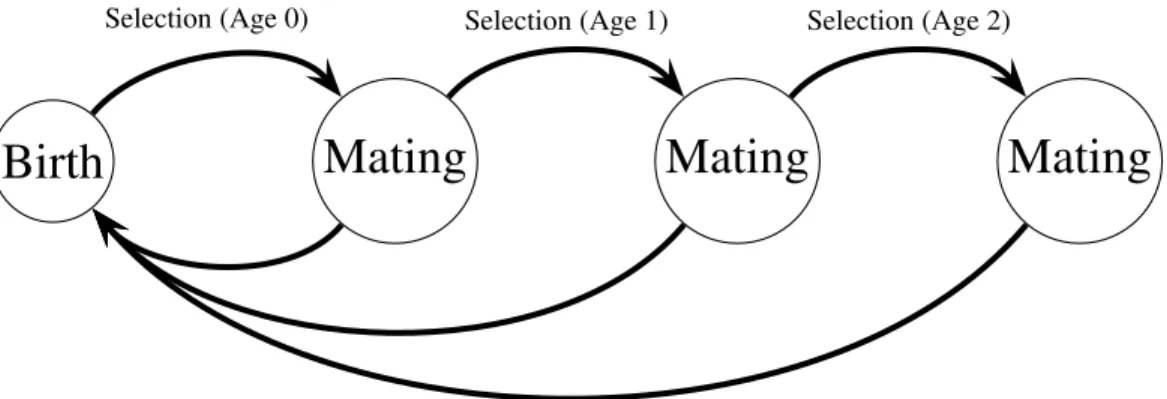
Selection (Age 0) Selection (Age 1) Selection (Age 2)Figure 2.1: Haploid life cycle for cohorts of males: haploid males emerge, grow, undergo selection, then mating, then repeated episodes of selection and mating. Meiosis then produces new zygotes following mating. Mutation in condition loci occurs before selection.
model uses a haploid life cycle (Figure 2.1): new zygotes arise from meiosis and undergo viability selection followed by mating. Males that survive the first round of selection and mating proceed to another round of selection and mating, and so on. Males provide no direct benefits to females, and can mate with multiple females. Each female mates once and lives for one episode of viability selection followed by mating. I assume a large population size so that we can ignore the effects of genetic drift. All male mortality results from selection on the trait and condition phenotypes except for males in the terminal age class, who are removed from the simulation unconditionally (see Equation (2.10)). Similarly, females do not suffer costs of choice, and all selection on females reflects selection on condition.
The model genome consists of five diallelic loci: two “condition” or “intrinsic viability” loci (C), the trait locus (T), the preference locus (P) and the age-dependent mode of expression locus (F). I refer to alleles of interest, e.g. the preference or trait allele, or beneficial condition alleles, with the subscript 2, and denote their frequencies by lower-case p with a subscript corresponding to the locus. For example pP represents the frequency of the choosiness allele
P2. The alleles at the condition loci are either “beneficial” or “deleterious.” The number
mutation from beneficial to deleterious (C2→C1) occurs in condition loci at a rate of 0.001
per individual per generation; mutation occurs in the zygote stage, before the first round of selection (see Figure2.1 on the preceding page).
Males carrying the T1allele do not produce the trait, regardless of condition. Males produce
the trait if they have the trait allele T2. A male agedywith condition phenotypeCcarrying T2
has trait size
t(C,y) =beCy. (2.1)
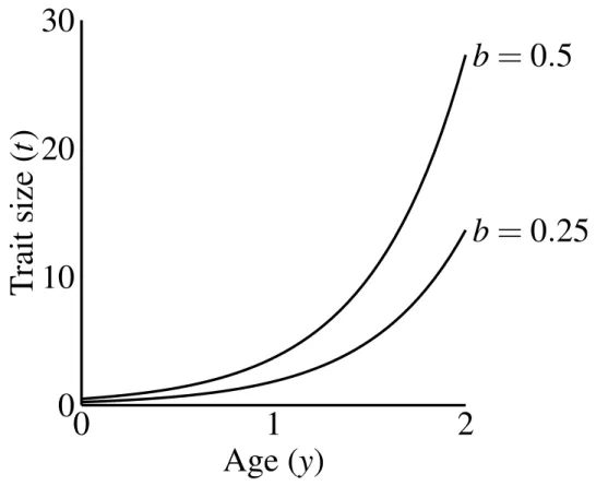
wherebis a parameter controlling the size of the trait, that I refer to as the “growth coefficient.” I chose this exponential function to emphasize three characteristics: (1) all males display the same trait size at age 0, as long as they carry the trait allele; (2) a large disparity in size between young and old males; and (3) simple scaling of the male trait size via the growth coefficient (b). Other trait functions do occur in nature (see Johnson and Hixon, 2011; Poissant et al., 2008), and could have different consequences for evolutionary dynamics (seeDiscussion on 20). Figure 2.2 on the next page shows that age-specific trait size linearly depends on the growth coefficient (the constant b). The growth coefficient linearly corresponds to the size of the trait across constant age and condition. A larger value ofb in a particular population (i.e. simulation) signifies that males of a particular genotype attain larger trait values than they would in populations with smallerb-values.
The P locus controls mate choice behavior of females. Mate choice occurs by relative pref-erence (as inKirkpatrick,1982) as a function of trait size. Females carrying P2encountering
a male with trait sizet areφ(t) =1+αt times more likely to mate than non-choosy females. Non-choosy females, carrying P1, mate randomly (φ(t) =1). The mating process normalizes
female mating frequency such that all females have equal mating success (see Equation2.5). In other words, all females mate in each mating cycle. Choosy females do not suffer any viability or opportunity costs.
The F locus controls mode of development. Males carrying the F1allele show age-dependent
0
10
20
30
0
1
2
Age (
y
)
Tr
ai
ts
iz
e
(
t
)
b
=
0
.
5
b
=
0
.
25
Figure 2.2: Male trait growth for high-condition males at two values of the growth coefficient, b=1.0 andb=0.5. Trait size at age 0 equalsb.
of three levels in a particular simulation: (1) t(C,0) =b, the trait value of a 0-year-old;
(2)t(C,ymax), the trait value of the oldest males in the population (still dependent on condi-tion); or (3) ¯t, the population mean trait value. The third set of simulations sought to create a population where age-independent (F2) males were of intermediate attractiveness, between
males the trait size ofbin Equation (2.1), as well as using the same indexing convention as the computer simulation. The number of age classes in the population isymax+1.
For the third set of simulations, where F2males carriedt=t, I updated ¯¯ t in every iteration.
My goal was ensuring that a class of males of intermediate attractiveness persisted in the pop-ulation. Therefore all males (regardless of condition) carrying F2received ¯tas their trait value
for a particular episode of mating, then I updated their values in the next iteration, following changes in ¯t. Furthermore, the value of ¯t used in these simulations reflected the full range of variation in condition, despite the lack of condition-dependence for F2 males. I therefore
calculated the mean trait as
¯ t= ∑
tmax
t=0t f(t,y)
ymax+1 (2.2)
where f(t,y) describes the frequency of males with trait value t at age y over ymax+1 age classes. The average is taken over all males, from unornamented males to the maximum trait size oftmax=beCymax, whereC represents the largest possible number of condition alleles (i.e. number of condition loci). Males carrying F2 contributed to the population mean as if their
traits were age-dependent, i.e. contributingt(C,y) =beCy to the calculation in Equation (2.2).
If the trait allele (T2) were to spread, then a contribution of ¯t by F2 males would depress
the trait value for F2 males and produce a delay in following phenotypic changes. Although
these procedures reduced biological realism from an individual perspective, they maintained the population genetic conditions relevant to the question at hand.
I used one level of expression per simulation, including simulations where the male pop-ulation was fixed for F2(an age-independent population). In a different set of simulations F2
initially occurred at a low frequency, comparable to the frequency of the trait, so that age-independent and age-dependent expression were in competition.
wm(C,t) =1+exp
−(C−C)
2 2µ2 +exp − t 2 2ν2 (2.3a)
wf(C) =
1+exp
−(C−C)
2
2µ2
(2.3b)
where males have C condition loci, µ sets the relative strength of selection for condition,
ν determines the relative strength of selection against the trait. Smaller values of µ and ν
correspond to stronger selection (see Figure2.3).
The frequency of haplotypes changes through viability selection:
P0
i(y) =Pi(Wy¯)W(yi)(y) (2.4)
wherePi(y)andPi0(y)represent the frequency of haplotypeiat ageybefore and after selection, respectively. Wi(y) correspondingly represents the viability of haplotypeiat age yand ¯W(y)
represents mean viability within age classy. The matrixMexpresses the probability of mating between a female of genotypeiand a male of genotype j:
Mi j= P 0
i∑yy=max0φi tj(y)
P0
j(y)π(y)
∑l∑yυmax=0φi(tl(υ))P
0
l(υ)π(υ)
(2.5)
whereπ(y)represents the frequency of males of agey, andtj(y) represents the trait size of a male of genotype j at agey. Condition is not an argument to thet() function in this case, as
it was in Equation (2.1) since the genotype j specifies the male’s condition. Equation (2.5) expresses the frequency of matings by summing over male ages the product of female mating rate (φ, a function of trait size) and the frequency of the male haplotype j in the general population, i.e. adjusted for the age structureπ. The subscription mating rate refers to choosy versus non-choosy females. The denominator adds up the age-dependent sums across all male haplotypes. The ratio of these summed terms then yields the probability that a male breeding with a female of haplotypeiis of haplotype j. Multiplying by the female haplotypeifrequency after selectionP0
Summing the product of mating probabilities and recombination probabilities across M yields the frequency of new zygotes
P0
i(0) =
∑
jkRjk→iMjk (2.6)
whereRjk→irepresents the proportion of jkmatings that yield genotypeiafter recombination (Bürger, 2000). Condition loci recombine freely (r =0.5) with each other and other loci;
other loci recombine at arbitrary frequencies (0≤ r≤ 0.5; see Table 2.1 on the following
page). Condition loci recombine freely so that they will represent unlinked loci far away in the genome, and could also represent multiple unlinked loci (Rowe and Houle,1996). The trait and preference loci recombine at arbitrary frequency since prior works show that recombination frequency affects indirect selection on preference (Kirkpatrick and Barton,1997;Kirkpatrick, 1982).
The relative size of the zygote class is found by the age-weighted sum of the mean fecun-dities of all adult age classes:
π0(0) = ymax
∑
y=0
¯
m(y)π(y) (2.7)
wherem(y)is the fecundity of an individual agedy. The new relative size of an adult age class
is given by the mean viability of the age class:
π0(y) =W¯(y)π(y) (2.8)
=π(y)
∑
iPi(y)Wi(y). (2.9)
I then calculate the new age distribution by dividing by the sum of all new age class sizes (Moorad and Promislow,2008):
π00(y) = π
0(y) ∑ymax
υ=0π
0(υ). (2.10)
I calculated the initial age structure by specifying λ, the geometric rate of increase for a population in stable age distribution. I then used this Gaussian survivorship function centered at 0 to calculate survival probabilities:
l(y) =exp
−y2
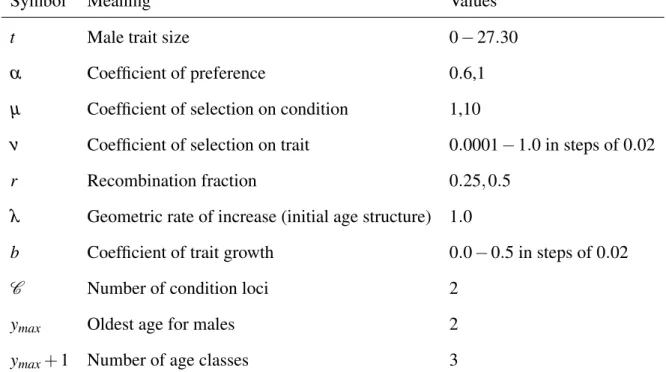
Symbol Meaning Values
t Male trait size 0−27.30
α Coefficient of preference 0.6,1
µ Coefficient of selection on condition 1,10
ν Coefficient of selection on trait 0.0001−1.0 in steps of 0.02
r Recombination fraction 0.25,0.5
λ Geometric rate of increase (initial age structure) 1.0
b Coefficient of trait growth 0.0−0.5 in steps of 0.02
C Number of condition loci 2
ymax Oldest age for males 2
ymax+1 Number of age classes 3
Table 2.1: List of variables and parameters with typical values
The age distribution is then given by (seeCharlesworth,1994):
π(y) = λ
−yl(y) ∑ymax
υ=0λ
−υl(υ). (2.12)
All simulations started with the trait allele T2and preference allele P2at non-zero
frequen-cies in the youngest age-class, and zero in the older age-classes. Simulations ran until: (1) the trait allele T2fixed; (2) the trait allele T2 or preference allele P2 was lost (frequency dropped
below 10−12); (3) the preference allele P
2fixed; (4) the Euclidean distance between successive
generations in preference and trait allele frequencies dropped below 10−9; or (5) the simulation
ran for 10 million iterations.
2.3 Results
Selection on male trait and growth
the same size as the eventual size of the age-dependent trait. Age-dependent simulations ran with coefficient of preference (α), recombination frequency (r) and selection on condition (µ) at the values indicated in Table 2.1 on the previous page. I used initial values of pC =0.01, pP=0.1, pT=0.001, andpF=0.0. I compare this to a population where all initial values were
the same except that males were fixed for F2, i.e. male trait expression was age-independent
and expressed at the largest size attainable (t=bexp(Cymax)). I analyzed the relative roles of selection intensity and trait size by plotting the equilibrium value of pT(fixation versus loss of
the trait allele) over a plane defined by 0.00001≤ν≤1.0 and 0≤b≤0.5 (see Table2.1; see Figures2.4 on page 27and 2.6).
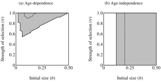
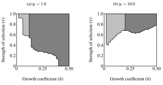
The area of parameter space where the trait fixes depends on three parameters: α (strength of preference), b(“growth coefficient”; see Equation (2.1)) andν (strength of selection; Fig-ure2.4 on page 27). Recombination frequency (r) and selection on condition (µ) do not appear to qualitatively affect the results in these simulations. Strength of preference affects the “readi-ness to mate” of females over the range of trait values present in these simulations: when
α =0.6 a choosy female is 9.20 times more likely to mate with a 2 year-old, high-condition
male with a growth coefficient of b=0.25. At the higher value of α =1.0, a choosy female is 14.65 times more likely to mate with the same trait-bearing male. We see a qualitative
dif-ference between populations with age-dependent traits and populations with age-independent traits at both values of α. The selection parameter ν determines the pattern of fixation for age-dependent traits, but has no effect on age-independent traits. Atα =0.6 the trait fixes in a very small portion of theb−ν plane nearν =1.0 in age-dependent simulations. The traits fixes above the thresholdbvalue of 0.20 in the corresponding age-independent simulations. At
α=1.0 the regions of fixation are larger, but the qualitative differences between age-dependent
(Fig-ure2.4b).
Figure2.5 on page 28shows a sample of linkage disequilibrium trajectories from the four regions defined by fixation and loss of age-dependent and age-independent traits. Each point on a curve represents the statistical association (linkage disequilibrium) between a beneficial condition allele and the ornament allele. A positive association indicates that the trait allele occurs in the same genotype with a beneficial condition allele more often than expected by chance. A negative association indicates that the two alleles are found less often in one geno-type than expected by chance. When the alleles randomly associate e.g. at the beginning of the simulation, or when one or both alleles are fixed or lost, the linkage disequilibrium equals zero. Condition alleles do not fix in these simulations due to biased mutation.
These associations indicate the effect of selection on genotypes that act as indicators of condition, i.e. have both a condition allele and a trait allele. When selection favors condition (always) and does not favor the trait, it will drive alleles apart so that they are rarely found in the same genotype, leading to the negative associations found in Figure2.5 on page 28. I caution the reader against interpreting the values in Figure2.5 on page 28as directly indicative of the strength of overall selection, since the quantities do not include adjustment for age structure. Each point reflects the action of selection on a particular cohort, and not the strength of selection against the trait in the population. For example, the larger absolute values in older age-classes in the figure does not indicate that selection acts more strongly on individuals in that age class. Selection works quite weakly on older age classes, since old individuals are quite rare.
classes, are less likely to be ornamented. However, this effect is generally much weaker in age-dependent populations than in age-inage-dependent populations (Figure2.5a on page 28). Males that reach the oldest age class under age-dependence are more likely to be high-condition and ornamented than under age-independence. More raw material for sexual selection remains within a cohort under age-dependence.
The right-hand column of Figure2.5 on page 28 shows trajectories for a larger trait (b=
0.2). A similar curve appears for age-dependent traits in Figure 2.5b on page 28 as in
Fig-ure2.5a on page 28. However, the age-independent trait responds to selection rapidly, showing a different shape from age-dependent populations (Figure2.5c on page 28 and Figure 2.5d). Readers should keep in mind when viewing this figure that the age structure of the population, especially under strong selection, biases heavily toward young males. Although linkage dise-quilibrium increases in older age classes, the associations for age class 0 most closely reflect the overall linkage disequilibrium in the population as a whole.
Mode of development
Another set of simulations sought to determine the crucial parameters favoring age-dependent expression over age-independent expression. These simulations began with polymorphism at the F locus, i.e. F2began at a low, non-zero frequency. Fixation of F2depended on the level of
trait expression chosen for the age-independent males in that simulation, one of (1)b; (2) ¯t; or (3)tmax=bexp(Cymax). I simulated these conditions with initial values ofpC=0.01, pP=0.1,
pT =0.1, and pF =0.1 in all age classes. Age-independent males occurred with one
partic-ular trait function (t =b, t =t, or¯ t =bexp(Cymax)) for a specific simulation: when the F2
allele caused males to have smaller traits than the oldest age-dependent males then F2was lost
everywhere in theb-ν-plane.
When males carrying F2expressed the trait range of the oldest age-dependent males
through-out their lives (t =bexp(Cymax)) the F2allele fixed in an area including the highest intensity
initial trait values where the trait did fix. In other words, expression remained polymorphic in this region, with the majority of males displaying age-dependence (light gray in Figure2.6a on page 29). This effect is even stronger when selection on condition is relaxed (µ=10; see
Fig-ure2.6b on page 29). The area of trait fixation where F remained polymorphic is larger when
µ =10 and includes regions of more intense selection against the trait as well as requiring
larger trait sizes for fixation of F2. Age-dependence occurs at larger trait sizes and under more
intense selection when the population displays more variance in condition. This suggests that for a givenb, age-independence only brings males a mating advantage with strong selection on condition.
I also repeated the above simulations with pF =0.9 initially. For all parameter values T2
was lost below a certain threshold value and above this threshold, both T2 and F2fixed. This
reinforces the above results: when the majority of males display age-independent expression, trait size alone determines the fixation of the trait.
Another set of simulations considered the fixation of the F2 allele with established traits
(pT=1.0) and preferences (pP=1.0; Figure2.7 on page 30). The F2allele was initially rare
(pF=0.1). Individuals carrying F2displayed the maximum trait size of age-independent males
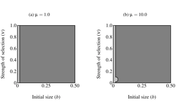
of comparable condition at their maximum age (t =bexp(Cymax)). Age-independent signal-ing came to predominate regardless of selection strength above a certain small size threshold. Below this threshold we can say that age-dependent signaling persisted. The same pattern was observed with a minor exception under strong selection against the trait, regardless of selection on condition (Figure2.7b on page 30): selection on condition does not appear to qualitatively affect the size at which age-independent signaling out-competes age-dependent signaling.
2.4 Discussion
selection can easily eliminate them. I have shown that an age-dependent trait can evolve under relatively weak selection at a wider range of trait sizes than can an age-independent trait (Fig-ure2.4 on page 27). While an age-dependent trait can evolve by producing small traits at young ages when selection is intense, larger initial trait sizes can only occur under proportionally less intense selection. This contrasts strongly with the age-independent simulations. Size of the trait determines the eventual fixation of the age-independent trait allele, regardless of selection intensity. Simulations with genetic variation for mode of development (dependent vs. age-independent) show that age-independence only evolves at larger trait sizes and age-dependence can predominate under weaker selection at smaller trait sizes. Invasion of age-independent traits occurred at relatively smaller trait sizes than when increasing from rarity. Again this only depended on trait size. Evolution of age-independence generally depends on trait size and not on the intensity of selection against the trait.
Altogether the simulations show that small traits in young males “solve” the dynamical problem of reduced heritability. The results suggest that three factors favor the evolution of age-dependent sexual signals: (1) low adult male mortality; (2) weak selection against the trait; and (3) strong age-dependence, i.e. small initial trait sizes. This result makes sense from a life-history strategy perspective. When adult mortality is lower, young males will invest less in reproductive strategies, producing a negative correlation between expected future repro-duction and age-specific investment. Males can afford to invest in mate attraction when adult mortality is low. Age-dependence effectively partitions the life-history of males into two stages dominated by two different fitness components. Viability takes precedence at young ages and mating success becomes more important later in life. This result parallels recent work on an abundant primate showing that juvenile survival followed by mating success form the most crucial fitness components (Courtiol et al.,2012).
within age-dependent traits, it can pass through to older age classes where it will be fully expressed. As males age they reveal additive variance in condition, thus making them more reliable signalers (as in Proulx et al.,2002). The trajectories illustrate how selection can only eliminate the age-dependent trait when either selection acts strongly or when the young-age trait is large enough. Weak selection (the top row of Figure2.5 on page 28) works even weaker on age-dependent populations, so as to barely change allele frequencies until males get older. Age-dependence weakens selection against the trait.
at-tractiveness in Figure2.4b on page 27where age-independent males show large enough traits to avoid this cost. Kokko(2001) has already noted that sexual advertisements are life-history traits. Considering the costs and benefits of advertisements requires evaluation of the entire life cycle and all the organism’s interactions and requirements (Badyaev and Qvarnström,2002).
The results here support the strategic modeling literature of age-dependent signals (Rands et al., 2011; Proulx et al., 2002; Kokko, 1997). Proulx et al. modeled the situation where male longevity and reproductive opportunities increase — e.g. under a low adult mortality en-vironment — and found that high-condition males downplay their signaling relative to lower condition males, preserving resources for survival. Kokkocame to the similar conclusion that young males of lower condition should signal more than their higher-condition cohorts, thus obscuring the observed relationship between genetic quality and trait value. Both studies find that (optimally) males of a given condition signal inversely proportional to number of remain-ing reproductive attempts (a predictor of condition in any age-class). Selection then favors females that prefer to mate with older males, since they are more likely to be of high condition. These studies model competing strategies, whereas my study uses a condition-dependent and age-dependent trait function to model variation. When selection weakens enough, with a par-ticular developmental trajectory, age-dependent signaling and female preferences evolve in a population genetic model. The evolutionary dynamics, in this case, do mirror the conclusions of the optimization models. These results suggest that with the needed life-history conditions and genetic variation we can expect selection on life-histories to produce age-dependent sig-naling.
Ja-cob et al., 2007; Miller and Brooks, 2005; Candolin, 2000a,b) and insects (Verburgt et al., 2011; Judge, 2011; Kivleniece et al., 2010; Jones and Elgar, 2004; Jones et al., 2000). De-spite the demographic problems of age-dependence, widespread occurrence of age-dependent traits suggests that life-histories promoting age-dependence are common. Body size or traits directly correlated with body size (e.g. weapons and ornaments) form the most obvious ex-ample of age-dependent traits, and should satisfy the assumptions of my model. Researchers found age-dependent sexual selection based on body size in Rocky Mountain Bighorn Sheep (Ovis canadensis;Coltman et al. 2002), who show a typical life-history characterized by weak-ening viability selection and increasing heritability over the lifespan. Older males pay less of a survival cost for larger bodies and larger horn sizes, facilitating greater success in mating competition. Certain behavioral and social traits should display age-dependence under weak natural selection, such as social network connectivity (McDonald and Potts, 1994) and song repertoire (Gil et al.,2001). Age-based honesty also creates an effective constraint producing age-dependence. High-condition males cannot bypass age-dependence by “faking” the trait. Certain “skills” such as nest-building (Evans,1997) show this form of honesty.
(a)µ=10,ν=1
2
.
0
3
.
0
4
.
0
5
.
0
0
1
2
1
2
t
C
(b)µ=10,ν=0.1
2
.
0
3
.
0
4
.
0
5
.
0
0
1
2
1
2
t
C
(c)µ=1,ν=1
2
.
0
3
.
0
4
.
0
5
.
0
0
1
2
1
2
t
C
(d)µ=1,ν=0.1
2
.
0
3
.
0
4
.
0
5
.
0
0
1
2
1
2
t
C
Figure 2.3: Fitness surfaces for males bearing ornaments: fitness slopes away from its max-imum at t =0 as the trait grows, and increases with more condition alleles. Decreasing µ decreases fitness for males with fewer than 2 condition alleles. When selection on condition weakens (µ =10, (a)and(b)) the fitness profile flattens in theC-dimension; compare this to
(a) Age-dependence
0 0.2 0.4
0.6
0.8
1.0
0 0.25 0.50
Initial size (b)
St re ng th of se le ct io n ( ν ) (b) Age-independence 0 0.2 0.4
0.6
0.8
1.0
0 0.25 0.50
Initial size (b)
St re ng th of se le ct io n ( ν )
Figure 2.4: Region of trait fixation (light gray) for age-dependent(a)and age-independent traits (b)in a plane defined by strength of selection against the trait (ν) and the growth coefficient of the trait (b). Dashed line indicates region of fixation underα=0.6; solid lines indicates region of fixation forα =1.0. The region of fixation for α =0.6 is contained within the region of fixation forα=1.0 in both panels. Under age-dependencebis the value of the trait for a 0-year old male. Theb-axis corresponds linearly to the trait size of ornamented males (t(C,y) =beCy),
(a)b=0.1,ν=0.8 -0.0045 -0.004 -0.0035 -0.003 -0.0025 -0.002 -0.0015 -0.001 -0.0005 0 0.0005
0 10 20 30 40 50 60
Linkage disequilibrium Generations Age-dependent Age 0 Age 1 Age 2 Age-independent Age 0 Age 1 Age 2
(b)b=0.2,ν=0.8
-0.006 -0.005 -0.004 -0.003 -0.002 -0.001 0 0.001 0.002 0.003
0 10 20 30 40 50 60
Linkage disequilibrium Generations Age-dependent Age 0 Age 1 Age 2 Age-independent Age 0 Age 1 Age 2
(c)b=0.1,ν=0.2
-0.004 -0.0035 -0.003 -0.0025 -0.002 -0.0015 -0.001 -0.0005 0 0.0005
0 10 20 30 40 50 60
Linkage disequilibrium Generations Age-dependent Age 0 Age 1 Age 2 Age-independent Age 0 Age 1 Age 2
(d)b=0.2,ν=0.2
-0.0015 -0.001 -0.0005 0 0.0005 0.001
0 10 20 30 40 50 60
Linkage disequilibrium Generations Age-dependent Age 0 Age 1 Age 2 Age-independent Age 0 Age 1 Age 2
(a)µ=1.0
0 0.2
0.4 0.6
0.8
1.0
0 0.25 0.50
Growth coefficient (b)
St re ng th of se le ct io n ( ν )
(b)µ=10.0
0 0.2
0.4 0.6
0.8
1.0
0 0.25 0.50
Growth coefficient (b)
St re ng th of se le ct io n ( ν )
Figure 2.6: Regions of fixation for the trait only (light gray) and the trait along with age-independent mode of development allele (F2; dark gray). Panel (a) shows strong selection
on condition and panel(b) shows weak selection on condition. The trait is lost in the white region. F2 does not change from its initial frequency of 0.1 in the light gray region, resulting
(a)µ=1.0
0 0.2
0.4 0.6
0.8
1.0
0 0.25 0.50
Initial size (b)
St re ng th of se le ct io n ( ν )
(b)µ=10.0
0 0.2
0.4 0.6
0.8
1.0
0 0.25 0.50
Initial size (b)
St re ng th of se le ct io n ( ν )
Figure 2.7: Regions of fixation for the age-dependent trait (light gray) and the age-independent trait (F2; dark gray) with the trait and preference initially fixed. Panel(a)shows strong selection
on condition and panel(b) shows weak selection on condition. The F2 allele supplants
CHAPTER 3: CONCLUSIONS 3.1 The basic problem or the basic opportunity?
Most individuals in growing populations are young. As individual viability selection in-creases lifespan, the proportion of the population present in older age classes inin-creases without changing this basic fact. Most of the genetic variance in fitness will still reside with younger individuals. However, as lifespan increases, old-age variance in fitness can occur more often than it does under shorter generation times. Alleles for late-acting variance in fecundity can come to predominate the younger age classes without becoming subject to selection. Such traits could evolve as long as they do not produce lower fitness in offspring, i.e. as long as genetic correlations between old-age fecundity and young-age survival remain non-negative.
Sexual signals must balance attractiveness with survival costs. Darwin’s original concept of sexual selection pointed out that traits bearing large costs could evolve for aesthetic or contest purposes (Ruse,1979). Any fitness benefit derived from mating must balance costs of carrying the trait. Recent models of sexual selection point out that realized fitness costs vary between individuals based on their intrinsic quality. However, the compensatory principle remains the same (Kokko et al.,2006). This raises particular problems for large morphological traits that require time to grow. Viability selection may favor a secondary sexual signal that grows slowly. The same trait could carry little value in attracting mates or deterring rivals.
fecundity then they can come to predominate in the younger age classes without being subject to strong viability selection. I therefore hypothesized that “demographic weakening” of selec-tion facilitates sexual selecselec-tion. I predicted that exaggeraselec-tion of sexual signals will be more likely to occur when traits depend on age. My analyses attempted to test these hypotheses by showing the characteristics of sexual selection under extended lifespan, and with particu-lar kinds of traits. The most basic task was demonstrating the conditions for evolution of an age-dependent trait. Smaller size and weaker selection did enable trait exaggeration, just as hypothesized (Chapter2).
I dealt with the question of the initial conditions that would differ between an age-dependent trait and a trait that appears independently of age. I investigated this question using a numerical simulation of a haploid population with a condition-dependent male trait, a female preference and varying modes of expression (see Section2.2 on page 9). Some simulations used wholly age-dependent expression, wherein any male bearing the trait expressed a larger trait as he grew older. Other simulations tested the conditions for evolution of a trait independent of age (see Section2.3 on page 16. Another set of simulations included both age-dependent and age-independent traits in the same population (see Section2.3 on page 19).
3.2 Implications for sexual selection
The conclusions of these investigations show that life-history plays a specific role in sexual selection. Previous calls for incorporation of life-history information into sexual selection have been primarily empirically focused (Badyaev and Qvarnström,2002, e.g.). Whereas multiple theorists have called for more detailed explorations of the implications of life-history theory (Trivers,1972;Partridge and Endler,1987;Kokko,2001), coverage in evolutionary theory has been limited to specific mechanisms. Hansen and Price(1995) stimulated a number of studies with the hope of clarifying intuitive ideas about age as an indicator mechanism (reviewed in Brooks and Kemp,2001).
REFERENCES
Adamson, J. J. (2013a, December). Evolution of female choice and age-dependent male traits with paternal germ-line mutation. arXiv:1312.3206 [q-bio].
Adamson, J. J. (2013b). Evolution of male life histories and age-dependent sexual signals under female choice. PeerJ In Press.
Badyaev, A. V. and A. Qvarnström (2002, April). Putting sexual traits into the context of an organism: A life-history perspective in studies of sexual selection. Auk 119(2), 301–310. Ballentine, B. (2009). The ability to perform physically challenging songs predicts age and
size in male swamp sparrows,Melospiza georgiana. Animal Behaviour 77(4), 973 – 978. Beck, C. (2002). A genetic algorithm approach to study the evolution of female preference
based on male age. Evolutionary Ecology Research 4(2), 275.
Beck, C. and L. Powell (2000). Evolution of female mate choice based on male age: are older males better mates? Evolutionary Ecology Research 2, 107–118.
Beck, C. W. and D. E. L. Promislow (2007). Evolution of female preference for younger males. PLoS ONE 2(9), e939.
Bonduriansky, R. and C. E. Brassil (2005, September). Reproductive ageing and sexual selec-tion on male body size in a wild populaselec-tion of antler flies (Protopiophila litigata). Journal of Evolutionary Biology 18(5), 1332–1340.
Brooks, R. and D. Kemp (2001). Can older males deliver the good genes? Trends in Ecology & Evolution 16, 308–313.
Bürger, R. (2000). The Mathematical Theory of Selection, Recombination and Mutation. J. Wiley and Sons.
Candolin, U. (2000a, December). Changes in expression and honesty of sexual signalling over the reproductive lifetime of sticklebacks.Proceedings of the Royal Society of London. Series B: Biological Sciences 267(1460), 2425 –2430.
Candolin, U. (2000b, October). Increased signalling effort when survival prospects decrease: male-male competition ensures honesty. Animal Behaviour 60(4), 417–422.
Charlesworth, B. (1994). Evolution in age-structured populations(2nd ed.). Cambridge Uni-versity Press.
Clinton, W. L. and B. J. Le Boeuf (1993). Sexual selection’s effects on male life history and the pattern of male mortality. Ecology 74(6), 1884–1892.
Courtiol, A., J. E. Pettay, M. Jokela, A. Rotkirch, and V. Lummaa (2012, May). Natural and sexual selection in a monogamous historical human population. Proceedings of the National Academy of Sciences 109(21), 8044–8049.
Darwin, C. (1871). The descent of man. J. Wiley and Sons.
Evans, M. R. (1997). Nest building signals male condition rather than age in wrens. Animal Behaviour 53(4), 749 – 755.
Evans, S. R., L. Gustafsson, and B. C. Sheldon (2011, June). Divergent patterns of age-dependence in ornamental and reproductive traits in the collared flycatcher. Evolution 65, 1623–1636.
Fisher, R. (1930). The genetical theory of natural selection. Oxford: Clarendon Press.
Garamszegi, L. Z., J. Török, G. Hegyi, E. Szöllõsi, B. Rosivall, and M. Eens (2007, March). Age-Dependent expression of song in the collared flycatcher, Ficedula albicollis. Ethol-ogy 113(3), 246–256.
Geary, D. C. (2002, xx). Sexual selection and human life history. Advances in child develop-ment and behavior 30, 41–101.
Gil, D., J. L. S. Cobb, and P. J. B. Slater (2001). Song characteristics are age dependent in the willow warbler,Phylloscopus trochilus. Animal Behaviour 62(4), 689 – 694.
Hammerstein, P. (1998). What is evolutionary game theory? In L. A. Dugatkin and H. K. Reeve (Eds.), Game Theory and Animal Behavior, Chapter 1, pp. 3–15. Oxford University Press.
Hansen, T. and D. Price (1995). Good genes and old age: Do old mates provide superior genes? Journal of Evolutionary Biology 8, 759–778.
Hansen, T. F. and D. K. Price (1999). Age-and sex-distribution of the mutation load. Genet-ica 106(3), 251–262.
Hawkins, G. L., G. E. Hill, and A. Mercadante (2012). Delayed plumage maturation and delayed reproductive investment in birds. Biological Reviews 87(2), 257â ˘A¸S274.
Hiebert, S. M., P. K. Stoddard, and P. Arcese (1989). Repertoire size, territory acquisition and reproductive success in the song sparrow. Animal Behaviour 37(Part 2), 266 – 273.
Jacob, A., G. Evanno, B. A. Von Siebenthal, C. Grossen, and C. Wedekind (2010). Effects of different mating scenarios on embryo viability in brown trout. Molecular Ecology 19(23), 5296–5307.
Johnson, D. W. and M. A. Hixon (2011). Sexual and lifetime selection on body size in a marine fish: the importance of life–history trade–offs. Journal of Evolutionary Biology 24, 1653–1663.
Jones, A. and N. Ratterman (2009). Mate choice and sexual selection: What have we learned since Darwin? Proceedings of the National Academy of Sciences 106(Supplement 1), 10001. Jones, T. M., A. Balmford, and R. J. Quinnell (2000, Apr). Adaptive female choice for middle-aged mates in a lekking sandfly. Proceedings of the Royal Society of London. Series B: Biological Sciences 267, 681–686.
Jones, T. M. and M. A. Elgar (2004, Jun). The role of male age, sperm age and mating history on fecundity and fertilization success in the hide beetle. Proceedings of the Royal Society of London. Series B: Biological Sciences 271, 1311–1318.
Judge, K. A. (2011). Do male field crickets,Gryllus pennsylvanicus, signal their age? Animal Behaviour 81(1), 185 – 194.
Kirkpatrick, M. (1982). Sexual selection and the evolution of female choice. Evolution 36, 1–12.
Kirkpatrick, M. and N. H. Barton (1997, February). The strength of indirect selection on female mating preferences. Proceedings of the National Academy of Sciences 94(4), 1282–1286. Kivleniece, I., I. Krams, J. Daukste, T. Krama, and M. J. Rantala (2010, December). Sexual
attractiveness of immune-challenged male mealworm beetles suggests terminal investment in reproduction. Animal Behaviour 80(6), 1015–1021.
Kodric-Brown, A. and J. H. Brown (1984). Truth in advertising: The kinds of traits favored by sexual selection. The American Naturalist 124(3), 309–323.
Kokko, H. (1997). Evolutionarily stable strategies of age-dependent sexual advertisement. Behavioral Ecology and Sociobiology 41, 99–107.
Kokko, H. (1998). Good genes, old age and life-history trade-offs. Evolutionary Ecology 12, 739–750.
Kokko, H. (2001). Fisherian and good genes benefits of mate choice: how (not) to distinguish between them. Ecology Letters 4(4), 322–326.
Kokko, H., R. Brooks, J. M. McNamara, and A. I. Houston (2002). The sexual selection continuum. Proceedings of the Royal Society B: Biological Sciences 269(1498), 1331–1340. Kokko, H., M. D. Jennions, and R. Brooks (2006). Unifying and testing models of sexual
selection. Annual Review of Ecology, Evolution and Systematics 37, 43–66.
Lande, R. (1981, June). Models of speciation by sexual selection on polygenic traits. Proceed-ings of the National Academy of Sciences 78(6), 3721–3725.
McDonald, D. and W. Potts (1994). Cooperative display and relatedness among males in a lek-mating bird. Science 266, 1030–1032.
Miller, L. K. and R. Brooks (2005, November). The effects of genotype, age, and social environment on male ornamentation, mating behavior, and attractiveness. Evolution 59(11), 2414–2425.
Moorad, J. A. and D. E. L. Promislow (2008). A theory of age-dependent mutation and senes-cence. Genetics 179(4), 2061–2073.
O’Donald, P. (1980). Genetic models of sexual selection. Cambridge: Cambridge University Press.
Oh, K. P. and A. V. Badyaev (2010). Structure of social networks in a passerine bird: Conse-quences for sexual selection and the evolution of mating strategies. The American Natural-ist 176(3), E80–E89.
Partridge, L. and J. A. Endler (1987). Life history constraints on sexual selection. InSexual selection: testing the alternatives, pp. 265–277. John Wiley and Sons Ltd.
Pemberton, J., D. Coltman, J. Smith, and D. Bancroft (2004). Mating patterns and male breed-ing success. In T. Clutton-Brock and J. Pemberton (Eds.), Soay Sheep: Dynamics and se-lection in an island population, pp. 166–189. Cambridge, UK: Cambridge University Press. Poissant, J., A. J. Wilson, M. Festa-Bianchet, J. T. Hogg, and D. W. Coltman (2008). Quan-titative genetics and sex-specific selection on sexually dimorphic traits in bighorn sheep. Proceedings of the Royal Society of London. Series B 275, 623–628.
Proulx, S. R., T. Day, and L. Rowe (2002). Older males signal more reliably. Proceedings of the Royal Society B: Biological Sciences 269(1507), 2291–2299.
Rands, S. A., M. R. Evans, and R. A. Johnstone (2011, November). The dynamics of honesty: Modelling the growth of costly, sexually-selected ornaments. PLoS ONE 6(11), e27174. Rowe, L. and D. Houle (1996). The lek paradox and the capture of genetic variance by
con-dition dependent traits. Proceedings of the Royal Society of London. Series B: Biological Sciences 263(1375), 1415–1421.
Ruse, M. (1979). The Darwinian revolution: science red in tooth and claw. Chicago: Univer-sity of Chicago Press.
Taff, C. C., C. R. Freeman-Gallant, P. O. Dunn, and L. A. Whittingham (2011, March). Re-lationship between brood sex ratio and male ornaments depends on male age in a warbler. Animal Behaviour 81(3), 619–625.
Verburgt, L., M. Ferreira, and J. Ferguson (2011, January). Male field cricket song reflects age, allowing females to prefer young males. Animal Behaviour 81(1), 19–29.