THE IMPACT OF AIR POLLUTANT TRANSPORT ON AIR QUALITY
AND HUMAN HEALTH IN GLOBAL AND REGIONAL MODEL
APPLICATIONS
Ciao-Kai Liang
A dissertation submitted to the faculty at the University of North Carolina at Chapel Hill in partial fulfillment of the requirements for the degree of Doctor of Philosophy in the Department of Environmental Sciences and Engineering in the Gillings School of Global
Public Health.
Chapel Hill 2018
Approved by: J. Jason West Barbara Turpin William Vizuete Joshua Fu
iii
ABSTRACT
Ciao-Kai Liang: The impact of air pollutant transport on air quality and human health in global and regional model applications
(Under the direction of J. Jason West)
iv
v
ACKNOWLEDGEMENTS
I would like to thank those who have involved through my entire doctoral program and have made this dissertation possible. I sincerely grateful to my advisor, Dr. J Jason West, for his guidance, patience and generous support throughout my doctoral program. I am deeply grateful to him for giving me such a valuable chance to work in his research lab, for providing me an opportunity to work on interesting projects. He consistently allowed these papers to be my own work and steered me in the right the direction whenever he thought I needed it. I would also like to thank for all my Ph.D. committee members, Prof. Barbara Turpin, Prof. William Vizuete, Prof. Joshua Fu and Sergey Napelenok, for taking time out from their busy schedules to provide valuable feedbacks and insights on my research.
I would also like to acknowledge my two senior colleagues Raquel Silva for being patient and tremendously helpful with my health impact project and Yuqiang Zhang for technical support with all issues related to air quality modeling. I would also like to thank Chi-tsan Wang with whom I learn modeling skill and share the modeling knowledge together for my research project. I would also like to thank Prof. Hsin-Chih Lai’s research team with his student Li-Wei Lai and Prof. Der-Min Tsai for providing me meteorology output and SMOKE emission data for CMAQ model input to make the interesting project of the third and fourth chapter of this dissertation possible.
vi
TABLE OF CONTENTS
LIST OF TABLES ... ix
LIST OF FIGURES ... xii
LIST OF ABBREVIATIONS ... xviii
CHAPTER 1 – INTRODUCTION ... 1
1.1 The sensitivity due to transport of air pollution ... 1
1.1.1 Air pollution chemistry ... 2
1.1.2 Sensitivity analysis... 3
1.2 Ambient air pollution and health... 7
1.3 Research objective ... 10
CHAPTER 2 – HTAP2 MULTI-MODEL ESTIMATES OF PREMATURE HUMAN MORTALITY DUE TO INTERCONTINENTAL TRANSPORT OF AIR POLLUTION AND EMISSION SECTORS ... 13
2.1 Introduction ... 13
2.2 Methods... 16
2.2.1 Modeled O3 and PM2.5 surface concentration ... 16
2.2.2 Model evaluation ... 18
2.2.3 Health impact assessment ... 20
2.3 Results ... 24
2.3.1 Response of O3 and PM2.5 concentrations to 20% regional and sectoral emission reductions ... 24
2.3.2 Global mortality burden associated with anthropogenic air pollution ... 26
vii
2.3.4 Effect of sectoral reductions on mortality ... 30
2.4 Discussion ... 32
2.5 Conclusions ... 35
CHAPTER 3 – THE SENSITIVITIES AND CONTRIBUTIONS OF SURFACE OZONE OVER KAO-PING AIR BASIN IN TAIWAN TO GEOGRAPHICALLY-DISTRIBUTED ANTHROPOGENIC VOC AND NOX EMISSIONS AND IMPLICATIONS FOR MITIGATION POLICY... 51
3.1 Introduction ... 51
3.2 Methodology ... 54
3.2.1 Model settings and configuration... 54
3.2.2 Sensitivity experiments ... 57
3.2.3 CMAQ model performance evaluation ... 60
3.2.4 O3 sensitivity analysis ... 61
3.2.5 Uncertainty analysis of the emission inventory ... 62
3.3. Results ... 63
3.3.1 CMAQ model simulation evaluation ... 63
3.3.2 CMAQ-HDDM sensitivities to Taiwan domain-wide emissions and evaluation with respect to BFM ... 66
3.3.3 O3 sensitivity to regional precursor emissions ... 67
3.4 Discussion ... 75
3.5 Conclusion ... 78
CHAPTER 4 – PM2.5 SENSITIVITIES AND SOURCE CONTRIBUTIONS OF GEOGRAPHICALLY-DISTRIBUTED PRECURSOR EMISSIONS OVER KAO-PING AIR BASIN IN TAIWAN AND IMPLICATIONS FOR MITIGATION POLICY ... 97
4.1 Introduction ... 97
4.2 Methodology ... 101
viii
4.2.2 Sensitivity experiments ... 104
4.2.3 CMAQ model performance evaluation ... 106
4.2.4 PM2.5 sensitivity analysis ... 107
4.3 Results ... 108
4.3.1 CMAQ model simulation evaluation ... 108
4.3.2 CMAQ-DDM sensitivities to KPAB domain-wide emissions and evaluation with respect to BFM ... 111
4.3.3 Source PM2.5 contribution to regional precursor emissions ... 113
4.4 Discussion ... 118
4.5 Conclusion ... 120
CHAPTER 5 – CONCLUSIONS ... 139
5.1 Scientific findings ... 139
5.2 Uncertainty and future research ... 142
5.3 Policy implication ... 144
APPENDIX A - MULTI-MODEL ESTIMATES OF PREMATURE HUMAN MORTALITY DUE TO INTERCONTINENTAL TRANSPORT OF AIR POLLUTION – SUPPLEMENTAL MATERIAL ... 147
APPENDIX B - THE SENSITIVITIES AND CONTRIBUTIONS OF SURFACE OZONE OVER KAO-PING AIR BASIN IN TAIWAN TO GEOGRAPHICALLY-DISTRIBUTED ANTHROPOGENIC VOC AND NOX EMISSIONS AND IMPLICATIONS FOR MITIGATION POLICY – SUPPLEMENTAL MATERIAL ... 186
APPENDIX C - PM2.5 SENSITIVITIES AND SOURCE CONTRIBUTIONS OF GEOGRAPHICALLY-DISTRIBUTED PRECURSOR EMISSIONS OVER KAO-PING AIR BASIN IN TAIWAN AND IMPLICATIONS FOR MITIGATION POLICY - SUPPLEMENTAL MATERIAL ... 203
ix
LIST OF TABLES
Table 2.1 Population-weighted multi-model mean O3 (ppb) and PM2.5 concentration (μg/m3) for the 2010 baseline, for the 6-month O
3 season average of 1-hr. daily maximum O3 and annual average PM2.5, shown with the standard
deviation among models. ... 38
Table 2.2 Population-weighted multi-model mean change in O3 (ppb) in receptor regions due to 20% regional (NAM, EUR, SAS, MDE and RBU), sectoral (PIN, TRN and RES) and global (GLO) anthropogenic emission reductions, for the 6-month O3 season average of 1-hr. daily maximum. The diagonal, showing the effect of each region on itself, is underlined. All numbers are rounded to the nearest hundredth, and are shown with standard deviations
among models. ... 39
Table 2.3 Population-weighted multi-model annual average change in PM2.5 concentrations (μg/m3) in receptor regions due to 20% regional (NAM, EUR, SAS, MDE and RBU), sectoral (PIN, TRN and RES) and global (GLO) anthropogenic emission reductions. The diagonal, showing the effect of each region on itself, is underlined. All numbers are rounded to the nearest hundredth, and are shown with standard deviations among
models. ... 40
Table 2.4 Annual multi-model empirical mean O3- and PM2.5-related premature deaths with 95% CI from Monte-Carlo simulations in parenthesis (including uncertainty in baseline mortality rates, RRs and air pollutant concentration across models) in year 2010 baseline. All numbers are rounded to three significant figures or the nearest 100 deaths. Empirical
mean is the mean of 1,000 Monte Carlo simulations... 41
Table 2.5 Annual avoided multi-model empirical mean O3-related premature respiratory deaths with 95% CI from Monte-Carlo simulations in parenthesis due to 20 % regional (NAM, EUR, SAS, MDE and RBU), sectoral (PIN, TRN and RES) and global (GLO) anthropogenic emission reductions in each region and worldwide. The diagonal, showing the effect of each region on itself, is underlined. For regional reductions, we also the RERER (eq. 4) as the percent of total avoided deaths in each receptor region that result from foreign emission reductions, as well as the percent of global avoided deaths from emission reductions in each source region. All numbers are rounded to three significant figures or the nearest 10
x
Table 2.6 Annual avoided multi-model empirical mean PM2.5-related premature deaths (IHD+STROKE+COPD+LC) with 95% CI from Monte-Carlo simulations in parenthesis due to 20 % regional (NAM, EUR, SAS, MDE and RBU), sectoral (PIN, TRN and RES) and global (GLO) anthropogenic emission reductions in each region and worldwide. The diagonal, showing the effect of each region on itself, is underlined. For regional reductions, we also the RERER (eq. 4) as the percent of total avoided deaths in each receptor region that result from foreign emission reductions, as well as the percent of global avoided deaths from emission reductions in each source region. All numbers are rounded to three significant figures or the nearest
10 deaths. ... 43
Table 2.7 Comparison of O3 and PM2.5-related premature deaths attributable to PIN, TRN and RES emissions with previous studies. Results from this study (for 20% reductions) are multiplied by 5. For Silva et al. (2016), we combine results for “Energy” and “Industry” to represent PIN, and use “Land transportation” to represent TRN and “Residential & Commercial” to represent RES. For Lelieveld et al. (2015), we combine the “Power generation” and “Industry” sectors to represent PIN, and use “Land Traffic”
to represent TRN, and “Residential Energy” to represent RES. ... 44
Table 3.1 Episode average NOX and VOC emissions rate (ton/day) in each sensitivity
political region in October 1-31, 2010. ... 81
Table 3.2 Key model performance metrics for the hourly NO2, VOC and O3 at 15
monitoring sites in KPAB (Fig. 3.1c) during October 1-5, 2010. ... 82
Table 3.3 Statistical comparison of the average sensitivity coefficient of MDA8 O3 (ppb per 100% change in emissions) averaged over the KPAB domain to Taiwan domain-wide average ANOX and AVOC emissions, using BFM
and HDDM for October 1-5, 2010.. ... 83
Table 3.4 Simulated daily maximum 8-hour O3 concentrations averaged over the KPAB political region (Fig. 3.1b), and zero‐out source contributions from local and upwind ANOX and AVOC emissions, Taiwan domain-wide biogenic emissions, and initial and boundary conditions on each episode
day. ... 84
Table 4.1 Episode average anthropogenic primary PM2.5, SO2, NOX, NH3 and VOCS Emissions rate (ton/day) by defined sensitivity regions in December 1-31,
xi
Table 4.2 Key model performance metrics for the 24-hour average PM precursors (ppb), PM10 and PM2.5 mass and PM2.5 species (ug/m3) at 15 monitoring
sites and 3 supersites in KPAB (Fig. 4.1c) during 21-24 December, 2010. ... 124
Table 4.3 Statistical comparison of episode-average of 24-hour PM2.5 sensitivity coefficients (μg/m3 per 100% change in emissions) over the KPAB domain to Taiwan domain-wide precursor emissions, using BFM and DDM for
December 21-24, 2010. ... 125
Table 4.4 Simulated episode-average 24-hour PM2.5 concentration (μg/m3) and a decomposition of the zero-out source regional contributions (μg/m3) of anthropogenic precursor emissions estimated by eq. 17 during December 21-24 over three KPAB sites. The dominant PM2.5 precursor contributing to PM2.5 concentration from a given source area is highlighted in bold font.
xii
LIST OF FIGURES
Figure 2.1 Global difference in multi-model mean O3 concentrations (ppb) in 20% emission reduction scenarios relative to the baseline for the year 2010 in a) North America (NAM), b) Europe (EUR), c) East Asia (EAS), d) South Asia (SAS), e) Middle East (MDE), f) Russia/Belarus/Ukraine (RBU), g) Power and Industry (PIN), h) Transportation (TRN), i) Residential (RES) and j) Global (GLO), shown for the 6-mo. O3 season average of 1-hr. daily
maximum health relevant metric. ... 45
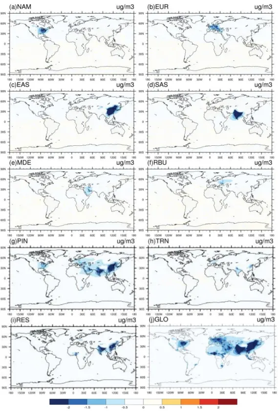
Figure 2.2 Global difference in multi-model annual mean PM2.5 concentrations (μg/m3) in 20% emission reduction scenarios relative to the baseline for the year 2010 in a) North America (NAM), b) Europe (EUR), c) East Asia (EAS), d) South Asia (SAS), e) Middle East (MDE), f) Russia/Belarus/Ukraine (RBU), g) Power and Industry (PIN), h)
Transportation (TRN), i) Residential (RES) and j) Global (GLO). ... 46
Figure 2.3 Annual avoided O3-related premature deaths in 2010 per 1,000 km2 due to20 % emission reduction scenarios relative to the base case in a) North America (NAM), b) Europe (EUR), c) East Asia (EAS), d) South Asia (SAS), e) Middle East (MDE), f) Russia/Belarus/Ukraine (RBU), g) Power and Industry (PIN), h) Transportation (TRN), i) Residential (RES) and j)
Global (GLO). ... 47
Figure 2.4 Annual avoided O3-related premature deaths in 2010 per million people due to 20 % emission reduction scenarios relative to the base case in a) North America (NAM), b) Europe (EUR), c) East Asia (EAS), d) South Asia (SAS), e) Middle East (MDE), f) Russia/Belarus/Ukraine (RBU), g) Power and Industry (PIN), h) Transportation (TRN), i) Residential (RES)
and j) Global (GLO)... 48
Figure 2.5 Annual avoided PM2.5-related premature deaths in 2010 per 1,000 km2 due to 20 % emission reduction scenarios relative to the base case in a) North America (NAM), b) Europe (EUR), c) East Asia (EAS), d) South Asia (SAS), e) Middle East (MDE), f) Russia/Belarus/Ukraine (RBU), g) Power and Industry (PIN), h) Transportation (TRN), i) Residential (RES)
xiii
Figure 2.6 Annual avoided PM2.5-related premature deaths in 2010 per million people due to 20 % emission reduction scenarios) relative to the base case in a) North America (NAM), b) Europe (EUR), c) East Asia (EAS), d) South Asia (SAS), e) Middle East (MDE), f) Russia/Belarus/Ukraine (RBU), g) Power and Industry (PIN), h) Transportation (TRN), i) Residential (RES)
and j) Global (GLO)... 50
Figure 3.1 (a) The four-level nesting modeling domains derived from WRF for the application of CMAQ. (b) The Taiwan domain, used for HDDM sensitivity analysis, defined by d04 at 3-km resolution (90 columns x 135 rows), and showing the five political regions for HDDM sensitivity analysis North and Chu-Miao Air Basin (NCMAB), Central Air Basin (CTAB), Yun-Chia-Nan Air Basin (YCNAB), Kao-Ping Air Basin (KPAB), and Yi-Lan and Hua-Dong Air Basin (YLHDAB) regions, where KPAB consists of the Kaohsiung and Ping-Tung administrative districts. The KPAB domain is shown as an orange rectangle (columns 15–55 and rows 1–70 of the Taiwan domain), and O3 concentrations are averaged over this region. (c) The locations of 15 monitoring sites are shown over part of KPAB (1.Daliao, 2.Xiaogang, 3.Renwu, 4.Zuoying, 5.Linyuan, 6.Qianjin, 7.Qianzhen, 8.Pingtung, 9.Hengchun, 10.Meinong, 11.Fuxing, 12.Nanzi, 13.Fengshan,
14.Chaozhou, 15.Qiaotou) ... 85
Figure 3.2 Synoptic surface weather maps for (a) 8am(LST) on 1 October, (b) 2pm(LST) on 1 October, (c) 8am(LST) on 2 October, (d) 2pm(LST) on 2 October, (e) 8am(LST) on 3 October, (f) 2pm(LST) on 3 October, (g) 8am(LST) on 4 October, (h) 2pm(LST) on 4 October, and (i) 8am(LST) on
5 October, 2010. ... 86
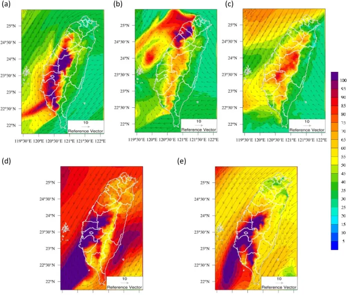
Figure 3.3 Simulated surface wind vectors and O3 concentration (ppb) over the Taiwan domain at 2pm (LST) on (a) 1 October (b) 2 October (c) 3 October (d) 4 October, and (e) 5 October, 2010. The reference vector on each plot
denotes a wind speed of 10 m/s. ... 87
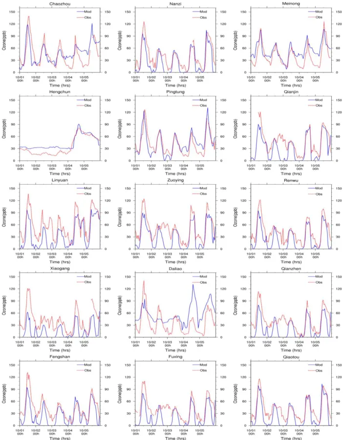
Figure 3.4 Time series of predicted hourly O3 concentration (ppb) concentrations compared with TAQMN measurements in KPAB (Fig. 3.1c) for October
1-5, 2010. ... 88
Figure 3.5 Hourly variations in pressure (hPa), temperature (0C), sunshine (%), relative humidity (%) and wind speed (m/s) at Kaohsiung station from
xiv
Figure 3.6 Spatial distribution of MDA8 O3 sensitivity coefficients (ppb per 100% change in emissions) shown over the KPAB domain (Fig. 3.1b) estimated by HDDM for ANOX and AVOC emissions from a) NAMAB b) CTAB c)
YCNAB d) YLHDAB and e) KPAB source regions on 1 October 2010. ... 90
Figure 3.7 a) Simulated daily maximum 8-hour O3 concentration (ppb) over the KPAB domain on 1 October 2010 for the base emission inventory, and HDDM zero-out source contributions (ppb) of anthropogenic ANOX and AVOC emissions combined from b) NAMAB c) CTAB d) YCNAB e) KPAB f) YLHDAB g) boundary conditions, and h) initial conditions. Note
that panels a, g and h have different color scales from panels b-f. ... 91
Figure 3.8 The 72-hour HYSPLIT backward trajectories (Red line) at the hour when the highest O3 concentration was observed on 1 October, 2010 at (a) Chaozhou (2pm)(b) Fengshan (12pm), along with trajectories 1 hour (purple), 2 hours (blue) and 3 hours (green) earlier. The site location is
shown with a yellow triangle. ... 92
Figure 3.9 Temporal variation in hourly O3 source contributions (ppb) of local and upwind anthropogenic precursor emissions and simulated and observed O3 concentration (ppb) during episode days at a)Chaozhou and b)Fengshan
site over KPAB. ... 93
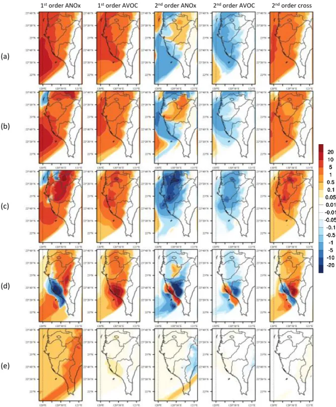
Figure 3.10. Hourly zero‐out source contributions (ppb) averaged over the KPAB political region for 1 October 2010 from upwind and local ANOx and AVOC emissions. S1NOX and S1VOC denote first‐order sensitivity coefficients, S2NOX and S2VOC denote minus one half of the second‐ order self-sensitivity coefficients, and S2CROSS are minus second‐order cross‐sensitivity coefficients, reflecting their contributions to the zero‐out source contribution in eq. 7. Each sensitivity coefficient in the legend is followed by N, C, Y, K, or I which indicates emissions from NCMAB, CTAB, YCNAB, KPAB and YLHDAB, respectively. The total simulated and observed O3 concentrations are shown on the right axis, and the source
contributions and sum of source contributions are shown on the left axis. ... 94
Figure 3.11 Isopleths of O3 (ppb) for the daily maximum 8-hour O3 concentration averaged over the KPAB political region on 1 October 2010 for changes in anthropogenic emissions from a) NCMAB, b) CTAB, c) YCNAB, d) KPAB and e) YLHDAB estimated by eq. 6. Axes reflect fractional changes
xv
Figure 3.12 Simulated sensitivities coefficient (ppb per 100% change in emissions) of the daily maximum 8-hour O3 averaged over the KPAB political region on 1 October, 2010 to local (KPAB) ANOX and AVOC emissions under the base emission inventory (thick black lines) and O3 sensitivity coefficient (ppb per 100% change in emissions) to various perturbations in the emission inventory for a) local ANOX from changes in local ANOX emissions, b) local AVOC from changes in local ANOX emissions, c) local ANOX from changes in local AVOC emissions, and d) local AVOC from
changes in local AVOC emissions. ... 96
Figure 4.1 (a) The four-level nesting modeling domains derived from WRF for the application of CMAQ. (b) The Taiwan domain, used for HDDM sensitivity analysis, defined by d04 at 3-km resolution (90 columns x 135 rows), and showing the five political regions for HDDM sensitivity analysis North and Chu-Miao Air Basin (NCMAB), Central Air Basin (CTAB), Yun-Chia-Nan Air Basin (YCNAB), Kao-Ping Air Basin (KPAB), and Yi-Lan and Hua-Dong Air Basin (YLHDAB) regions, where KPAB consists of the Kaohsiung and Ping-Tung of administrative districts. The KPAB domain is shown as an orange rectangle (columns 15–55 and rows 1–70 of the Taiwan domain), and is used to analyze ozone concentrations averaged over this region, and (c) The location of 16 monitoring sites are shown over KPAB (1.Daliao, 2.Xiaogang, 3.Renwu, 4.Zuoying, 5.Linyuan, 6.Qianjin, 7.Qianzhen, 8.Pingtung, 9.Hengchun, 10.Meinong, 11.Fuxing, 12.Nanzi, 13.Fengshan, 14.Chaozhou, 15.Qiaotou, 16. Fuying, where Fuying,
Qianzhen and Chaozhou are supersites.) ... 127
Figure 4.2 Synoptic surface weather maps for (a) 12am(LST) on 21 December, (b) 12pm(LST) on 21 December, (c) 12am(LST) on 22 December, (d) 12pm(LST) on 22 December, (e) 12am(LST) on 23 December, (f) 12pm(LST) on 23 December, (g) 12am(LST) on 24 December, and (h)
12pm(LST) on 24 December in 2010. ... 128
Figure 4.3 Simulated surface wind vectors and PM2.5 concentrations at (a) 12am(LST) on 21 December, (b) 12pm(LST) on 21 December, (c) 12am(LST) on 22 December, (d) 12pm(LST) on 22 December, (e) 12am(LST) on 23 December, (f) 12pm(LST) on 23 December, (g) 12am(LST) on 24 December, and (h) 12pm(LST) on 24 December in 2010. The reference
vector on each plot denotes a wind speed of 10 m/s. ... 129
Figure 4.4 Simulated KPAB domain-wide episode-average 24-hour surface PM2.5
xvi
Figure 4.5 Time series of predicted hourly PM2.5 concentration (μg/m3) concentrations compared with TAQMN measurements inside KPAB
domain for December 21-24, 2010. ... 131
Figure 4.6 Hourly variations in pressure (hPa), temperature (0C), sunshine (%), relative humidity (%) and wind speed (m/s) at Kaohsiung station from
Taiwan’s Central Weather Bureau during 21 to 24 December, 2010. ... 132
Figure 4.7 Spatial comparison between DDM (bottom) and BFM (top) for the 4-day episode average 24-hour PM2.5 sensitivity coefficients (μg/m3 per 100% change in emissions) over the KPAB domain (Fig. 1b) to Taiwan domain-wide anthropogenic primary PM2.5, SO2, NOx, NH3 and VOCs emissions during December 21-24, 2010. While BFM sensitivity coefficient is calculated by eq. 14 using ±10% emission perturbations, DDM sensitivity coefficient is calculated by eq. 15 using infinitesimal emission
perturbations. ... 133
Figure 4.8. Spatial distribution of the 4-day episode average PM2.5 sensitivity coefficients (μg/m3 per 100% change in emissions) in the KPAB domain to anthropogenic primary PM2.5, SO2, NOX, NH3 and VOCS emissions
from different source regions. ... 134
Figure 4.9 Four-day episode-average simulated and observed PM2.5 concentrations (μg/m3) and a decomposition of the zero-out source contributions (μg/m3) from local and upwind anthropogenic emissions at individual KPAB sites (Fig. 4.1c), the average of KPAB sites and averaged over the KPAB
political region (Fig. 4.1b). ... 135
Figure 4.10. A decomposition of 4-day episode average (a) PM2.5 and (b) PM2.5 species zero-out source contributions (μg/m3) from anthropogenic emissions of primary PM2.5, SO2, NOX, NH3 and VOCs from different
source regions by averaging over all KPAB sites (Fig. 4.1c). ... 136
Figure 4.11. Daily cycle of episode-average simulated and observed PM2.5 concentrations and a decomposition of the zero-out source contributions from local and upwind anthropogenic emissions (μg/m3) at a) Qiaotou
xvii
Figure 12. The 72-hour HYSPLIT backward trajectories a) at 8pm on 23 December at Qiaotou (background), b) at 9pm on 22 December at Qianzhen (urban) and c) 2pm on 22 December at Chaozhou (rural) when the peak PM2.5 was observed (i.e. at 0 hour), and the corresponding simulated total PM2.5 (μg/m3) and PM
2.5 source contributions (μg/m3) from local and upwind anthropogenic emissions and PM2.5 precursors i.e. primary PM2.5 (μg/m3), and NOx (ppb), VOCs(ppb), SO2 (ppb) and NH3 (ppb) concentration at each hour and location along the moving trajectory. The triangle in yellow
xviii
LIST OF ABBREVIATIONS
ACS American Cancer Society
AQMEII Air Quality Modelling Evaluation International Initiative
BC Black carbon
BC Boundary conditions
BFM Brute Force Method
CMAQ Community multiscale air quality model COPD Chronic pulmonary obstructive disease CRF Concentration response function CTAB Central Air Basin
CTM Chemical Transport Model
CWB Central Weather Bureau
DDM Decoupled Direct Method
DFW Dallas-Fort Worth
EAS East Asia
EDGAR Emission Data Base for Global Research
EMEP European Monitoring and Evaluation Programme
EPA Environmental Protection Agency
EUR Europe
FDDA Four-dimensional data assimilation GBD Global Burden of Disease
GFED Global Fire Emissions Database
GLO Global
H2O2 Hydrogen peroxide
xix
HNO3 Nitric acid
HR Hazard ratio
HYSPLIT Hybrid Single Particle Lagrangian Integrated Trajectory IC Initial conditions
IER Integrated Exposure-Response
IHD Ischemic heart disease
KPAB Kao-Ping air basin
LC Lung cancer
LRT Long range transport MAGE Mean absolute gross error
MB Mean bias
MCIP Meteorology/Chemistry Interface Processor
MDE Middle East
MEGAN Model of Emissions of Gases and Aerosols from Nature MICS-Asia Modelling Intercomparison Study-Asia
NAM North America
NAAQS National Ambient Air Quality Standards NCEP National Centers for Environmental Prediction NCMAB North and Chu-Miao Air Basin
NH3 Ammonia
NH4+ Ammonium
NMB Normalized mean bias
NME Normalized mean error
NO2 Nitrogen dioxide
NO3− Nitrate
xx
O3 Ozone
OC Organic carbon
PIN Power and Industry
PM2.5 Fine particulate matter with aerodynamic diameter <2.5 μm R Correlation coefficient
RBU Russia/Belarus/Ukraine
RERER Extra-Regional Emission Reduction
RES Residential
RESP Chronic respiratory mortality RMSE Root mean square error
RR Relative risk
SAS South Asia
SMOKE Sparse Matrix Operator Kernel Emissions SOA Secondary organic aerosol
SO2 Sulfur dioxide
SO42− Sulfate
SRRS Source-receptor relationships STROKE Cerebrovascular disease
TAQMN Taiwan Air Quality Monitoring Network TBEIS Taiwan Biogenic Emissions Inventory System TEDS Taiwan Emission Data System
TF-HTAP Task Force on Hemispheric Transport of Air Pollution TOAR Tropospheric Ozone Assessment Report
TRN Transportation
xxi YCNAB Yun-Chia-Nan Air Basin
1
CHAPTER 1 – INTRODUCTION
Ground-level ozone (O3) and fine particulate matter with aerodynamic diameter <2.5 μm (PM2.5) are major constituents of urban and regional smog and are suspected of affecting human health. As air pollution can travel long distance, ambient O3 and PM2.5 concentrations are determined not only by local emission sources but also by the transport of O3 and PM2.5 and their precursors. Understanding the response of air pollutant to the change in emissions from local and upwind emission region is therefore particularly important for a region to formulate effective emission control strategies to achieve O3 and PM2.5 attainment. In addition, as changes in emissions from one region influence air quality over others, they can also influence premature mortality in other regions. In this study, I investigate the sensitivity of O3 and PM2.5 concentrations to changes in precursor emissions, and the contribution from local and upwind emissions over Kao-Ping air basin (KPAB) located in the southwestern region of Taiwan. I also estimate the impacts of interregional transport on human premature mortality from regional and sectoral emission reductions, using an ensemble of global chemical transport models on an intercontinental scale.
1.1 The sensitivity due to transport of air pollution
2
pathway from the source to receptor and the pollutant transformation, production, and loss processes that occur along the pathway.
1.1.1 Air pollution chemistry
Ground-level O3 is a secondary air pollutant driven by photochemical reactions of volatile organic compounds (VOCs) and nitrogen oxides (NOX= NO + NO2). VOCs and NOX are O3 precursors and can arise from both biogenic and anthropogenic emission sources. The photochemical production of O3 depends on the availability of NOX and VOCs in a nonlinear manner (Cohan et al., 2005; NARSTO, 2000; Seinfeld et al., 2006). Changing emissions of NOX and VOCs can produce strong non-linear responses in O3 depending on the local relative abundance of NOX and VOCs. Under high NOX, low VOCs conditions such as in urban core areas, O3 production is inhibited and reductions of NOX can increase local O3 (often referred to as a VOC-limited regime). In the opposite case such as suburban and rural areas, O3 production is more efficient and reductions of NOX will decrease O3 (often referred to as a NOX -limited regime). Jin et al. (2008) showed that nitrogen oxides (NOx) emission reductions are overall more effective than VOCs control for attaining the 8 h O3 standard in San Joaquin Valley (SJV) of central California for a 5 day O3 episode, in contrast to the VOC control that works better for attaining the prior 1 h O3 standard. To meet National Ambient Air Quality Standards (NAAQS) for O3, Downey et al. (2015) proposed that 2006 anthropogenic NOX and VOCs emissions must be reduced by 60-70% to reach maximum daily average 8-h O3 of 75 ppb in Sacramento, St. Louis, and Philadelphia while Los Angeles requires 92% emissions reductions. Understanding the O3 non-linear sensitivity to precursor emissions is a key to developing effective abatement strategies on O3 in polluted regions.
3
PM2.5 components include ammonium, sulfates, and nitrates, secondary organic aerosol (SOA) which are produced from precursor gases (SO2, NOX, NH3 and VOCs) (Ansari et al., 1998; NARSTO, 2004; Seinfeld et al., 2006). Several chemical processes can form secondary PM2.5 from its precursor species. The oxidation of SO2 is an important process for formation of sulfate. Nitric acid (HNO3) is formed from NOX and the reaction of NH3 and HNO3 forms nitrate. NH3 is the primary basic species, forming ammonium (NH4+) in particles to neutralize acidic nitrate (NO3−) and sulfate (SO42− formed from SO2). The organic component of ambient particles is a complex mixture of hundreds or even thousands of organic compounds (Hallquist et al., 2009; Kroll et al., 2008). These organic compounds are either emitted directly from sources (primary organic aerosol) or can be formed in-situ by condensation of low-volatility hydrocarbon-oxidation products (secondary organic aerosol). As organic gases are oxidized by species such as OH, O3, and NO3, their oxidation products accumulate. Whereas secondary PM2.5 often responds linearly to its precursor emissions, this response could be nonlinear under some circumstances. PM2.5 concentrations can even increase as SO42− concentrations decrease, by allowing more HNO3 to condense (Ansari et al., 1998; West et al., 1999). A decrease in NOX may lead to an increase in nitrate concentrations because the increase in oxidant concentrations exceeds the decrease in nitrogen dioxide (NO2) concentrations (Pun et al., 2001). A reduction in VOCs emissions similarly leads to a reduction in PM organic compound concentrations but may lead to increases in sulfate and nitrate concentrations due to increases in oxidant concentrations and/or decreases in the formation of gaseous organic nitrates (Meng et al., 1997). To design effective PM2.5 control management strategy, it requires fully knowledge of how PM2.5 responds to changes in its precursors
1.1.2 Sensitivity analysis
4
relationships between source emissions and receptor concentrations. This calculation of SRRS can be classified into source-oriented and receptor-oriented approaches. The source-oriented approach is the most commonly-used approach, where emissions from a particular source region are perturbed and these perturbations are propagated forward in time throughout the model domain. In the receptor-oriented approach, the perturbation in the receptor region from a change in emissions is traced back in time through the model domain. Both are used to define how much individual source regions contribute to ground-level pollution, therefore the information from this SRRS can critically inform policy decision making. This study here will mainly focus on a source-oriented method for a SRRS estimate. Two techniques commonly used for SRRS evaluation are Brute Force Method (BFM) and Decoupled Direct Method (DDM).
BFM is the simplest way to evaluate the concentration response to the change in emission in Chemical Transport Model (CTM). In BFM, the emissions from the source region of interest are set to zero. The concentrations coming from the source region are then defined as the difference between a base case run and the zeroed-out run. Roselle et al. (1995) applied regional oxidant model to estimate the contribution of 17 different anthropogenic VOC and NOx emissions scenarios to zone in the eastern United States and Wang et al. (2015) applied BFM as a source sensitivity method for quantifying source contributions of PM2.5 in three cities by zeroing out emissions from different emission sectors. Traditionally, these questions of atmospheric sensitivity have been addressed with a BFM. BFM is simple; however, when it comes to model more SRRS scenarios, BFM becomes computational burdensome. For example, N pairs of SRRS modeling result requires conducting N+1 simulations. Furthermore, the BFM has been shown to be susceptible to numerical instability in small emission perturbation due to model discontinuities and round-off errors (Napelenok et al., 2006).
5
6 equations to derive sensitivities simultaneously.
7
originated from reactive nitrogen originally released upwind of the SJV. The effect of local emissions controls on this upwind material was small. Ying et al. (2009) showed that 68% of the particulate nitrate formed in the most polluted sub-regions of the Central Valley originates from emissions in those same sub-regions while local emissions controls is with regard to an effective strategy to reduce airborne particulate matter concentrations to acceptable levels. Shin et al. (2004) derive multiple source-receptor matrices to show inter- and intrastate impacts of emissions on both O3 and PM2.5 over the eastern United States and showed that local (in-state) emissions generally account for about 23% of both local O3 concentrations and PM2.5 concentrations, while neighboring states contribute much of the rest. Bergin et al. (2007) showed that an average of 77% of each state's O3 and PM2.5 concentrations that are found to be caused by emissions from other states where Delaware, Maryland, New Jersey, Virginia, Kentucky, and West Virginia are shown to have high concentrations of O3 and PM2.5 caused by interstate emissions. Understanding the relative importance of various nonlinearities and cross sensitivities can therefore facilitate interregional cooperation for air pollution mitigation.
1.2 Ambient air pollution and health
Epidemiologic studies looking at effects over large populations with statistical relationships between air pollutant concentrations and health outcomes have shown that both short-term and long-term exposures to O3 and PM2.5 are associated with elevated rates of premature mortality. Short-term temporal variation in concentrations of air pollution over days or weeks has been used to estimate effects on daily mortality and morbidity in time-series studies. They provide estimates of the increase in deaths brought forward in time by recent exposure. Spatial variation in long-term average concentrations of air pollution has provided the basis for cohort studies of long-term exposure. Cohort studies include not only those whose deaths were brought forward by recent exposure to air pollution, but also those who died from chronic disease caused by long-term exposure.
8
department visits and hospital admissions due to asthma exacerbation or other respiratory conditions and mortality (Bell et al., 2005; Bell et al., 2014; Gryparis et al., 2004; Ito et al., 2005; Levy et al., 2005; Stieb et al., 2009) while long-term exposure to O3 has been associated with premature respiratory mortality (Jerrett et al., 2009, Turner et al., 2016). Short-term exposure to PM2.5 has been associated with increases in daily mortality rates from all natural causes, and specifically from respiratory and cardiovascular causes (Bell et al., 2014; Du et al., 2016; Powell et al., 2015; Pope et al., 2011) while long-term exposure to PM2.5 can have detrimental chronic health effects, including premature mortality due to cardiopulmonary diseases and lung cancer (Brook et al., 2010; Burnett et al., 2014; Hamra et al., 2014; Krewski et al., 2009; Lepeule et al., 2012; Lim et al., 2012).
9
circulatory (HR = 1.03, 95% CI 1.01-1.05), and respiratory mortality (HR = 1.12, 95% CI 1.08-1.16) that were unchanged with further adjustment for NO2 in two pollutant models adjusting for PM2.5. For PM2.5, a recent new Integrated Exposure-Response (IER) model for premature mortality is associated with ischemic heart disease (IHD), cerebrovascular disease (stroke), chronic pulmonary obstructive disease (COPD), and lung cancer (LC) was proposed by Burnett et al. (2014). In this model, the CRF flattens off at higher PM2.5 concentrations relative to log-linear relationship of CRF by previous study (Kreswki et al., 2009), yielding different estimates of excess mortality for identical changes in air pollutant concentrations in low-polluted vs. highly-polluted locations and a uniform distribution from 5.8 μg/m3 to 8.8 μg/m3 is used for counterfactual concentration as suggested by Burnett et al. (2014).
Estimates of excess mortality due to air pollution can be obtained for total air pollutant concentrations above a counterfactual (zero or low-concentration threshold) or for anthropogenic air pollution (assuming a counterfactual that corresponds to natural air pollution or using output from modeling studies that exclude anthropogenic emissions). For example, the Global Burden of Disease Study 2015 (GBD 2015) estimated 254,000 deaths/year associated with ambient O3 and 4.2 million associated with ambient PM2.5 in which theoretical minimum risk exposure level was assigned a uniform distribution of 2.4–5.9 μg/m³ for PM2.5 and 33.3–41.9 ppb for O3 (Cohen et al. 2017). Silva et al. (2013) showed that exposure to present-day anthropogenic ambient air pollution is associated with 470,000 (95% confidence interval, 140,000 to 900,000) deaths/year from O3-related respiratory diseases, and 2.1 (1.3 to 3.0) million deaths/year from PM2.5-related cardiopulmonary diseases and lung cancer using modeled 1850 and 2000 concentrations from an ensemble of models (Silva et al., 2013).
10
PM2.5, and have estimated the effects of this LRT on premature mortality (Anenberg et al., 2009; Anenberg et al., 2014; Crippa et al., 2017; Duncan et al., 2008; Liu et al., 2009b; West et al., 2009b) while other studies have evaluated the relative importance of individual emissions sectors (Barrett et al., 2010; Bhalla et al., 2014; Chafe et al., 2014; Chambliss et al., 2014; Corbett et al., 2007) or multiple sectors (Lelieveld et al., 2015; Silva et al., 2016a) to ambient air pollution–related premature mortality. In general, above studies used global CTMs to represent LRT. While these coarse resolution CTMs are useful to represent LRT, their use for health impact analysis may cause uncertainties in concentrations and exposures near urban regions, where there are strong gradients in population density and pollutant concentrations and urban chemistry may modify the effects of LRT. In addition, all studies apply concentration-response relationships from epidemiological studies in industrialized nations (i.e. ACS) to the rest of the world. Despite those uncertainties, understanding of the extent to which changes in emissions outside a region affect the health impact within a given region in continental scale provide the incentive of reduce pollution transported over long distances through collective international cooperation.
1.3 Research objective
In this dissertation, I aim to investigate the response of air pollution and human health to change in emission due to air transport from model applications by answering the following questions:
1. How do anthropogenic emission reductions from one region influence health effects over other regions? (Chapter 2)
2. How do different anthropogenic sectoral emission reductions influence health effects spatially? (Chapter 2)
3. What is the response of O3 and PM2.5 to the change in local and upwind anthropogenic precursor emissions over KPAB? (Chapter 3 and 4)
11
O3 and PM2.5 attainment in KPAB? (Chapter 3 and 4)
In Chapter 2, I use output from the TF-THAP2 model ensemble to estimate annual O3- and PM2.5-related global cause-specific premature mortality and avoided mortality by 20% regional and sectoral emission reductions. A health impact function based on epidemiological relationships between ambient air pollution concentration and mortality was used in each grid cell with performing uncertainty analysis. This work has gone beyond previous TF-HTAP1 studies that quantified premature mortality from interregional air pollution transport, by using more source regions, analyzing source emission sectors, and using updated atmospheric models and health impact functions.
The effect of long-range transport of air pollution could also have impact on air quality outside of the interested region. In Chapters 3 and 4, I select Kao-Ping air basin (KPAB) located in the southwestern region of Taiwan to evaluate the impact of inter-basin transport of precursor emissions on O3 and PM2.5 air quality over the KPAB. The community multiscale air quality model (CMAQ) with decouple direct method (DDM) and high-order decouple direct method (HDDM) is used to investigate the sensitivity of PM2.5 and O3 concentrations to changes in local and upwind precursor emissions. Four layer nesting domain was performed with a resolution of 81/27/9/3 km nested on a Lambert conformal projection over East Asia. The model input of meteorology is driven by the Weather Research and Forecasting (WRF) model while emission inventory processed by Sparse Matrix Operator Kernel Emissions (SMOKE). To quantify the contribution from local and upwind anthropogenic emission, the Taylor expansion approximation is used to calculate the zero-out source contribution (ZOC) of local and upwind emissions by parametric scaling technique with sensitivity coefficients from HDDM and DDM. This work is first attempt to investigate the response of O3 and PM2.5 to local and specific upwind air basin emissions over the KPAB.
12
13
CHAPTER 2 – HTAP2 MULTI-MODEL ESTIMATES OF PREMATURE HUMAN MORTALITY DUE TO INTERCONTINENTAL TRANSPORT OF AIR POLLUTION
AND EMISSION SECTORS
2.1 Introduction
14
Numerous observational and modeling studies have shown that anthropogenic emissions can affect O3 and PM2.5 concentrations across continents (Dentener et al., 2010; Heald et al., 2006; Leibensperger et al., 2011; Lin et al., 2012; Lin et al., 2017; Liu et al., 2009a; West et al., 2009a; Wild and Akimoto, 2001; Yu et al., 2008). As changes in emissions from one continent influence air quality over others, several studies have estimated the premature mortality from intercontinental transport (Anenberg et al., 2009; Anenberg et al., 2014; Bhalla et al., 2014; Duncan et al., 2008; Im et al., 2018; Liu et al., 2009b; West et al., 2009b; Zhang et al., 2017). In 2005, the Task Force on Hemispheric Transport of Air Pollution (TF-HTAP) was launched under the United Nations Economic Commission for Europe (UNECE) Convention on Long-Range Transboundary Air Pollution (LRTAP). One of its tasks is to investigate the impacts of emission reductions on the intercontinental transport of air pollution, air quality, health, ecosystem and climate effects, using a multi-model ensemble to quantify uncertainties due to differences between models (Anenberg et al., 2009; Anenberg et al., 2014; Fiore et al., 2009; Fry et al., 2012; Huang et al., 2017; Stjern et al., 2016; Yu et al., 2013).
15
lifetime of O3 and its relatively larger scale of influence, PM2.5 was found to cause more deaths from intercontinental transport (Anenberg et al., 2009; 2014). These prior studies have consistently concluded that most avoided O3-related deaths from emission reductions in NAM and EUR occur outside of those regions, while most avoided PM2.5-related deaths occur within the regions. Similarly, an ensemble of regional models in the third phase of the Air Quality Modelling Evaluation International Initiative (AQMEII3) found that a 20% decrease of emissions within the source region avoids 54,000 and 27,500 premature deaths in Europe and the U.S. (from both O3 and PM2.5), while the reduction of foreign emissions alone avoids ~1,000 and 2,000 premature deaths in Europe and the U.S. (Im et al., 2018). Crippa et al (2017) used the TM5-FASST reduced-form model with HTAP2 emissions to estimate a global sensitivity to 20 % emission reductions of PM2.5-related premature deaths of 401,000 globally, and 42,000 and 20,000 for Europe and the US respectively.
16
In this study, we estimate the impacts of interregional transport and of source sector emissions on human premature mortality from O3 and PM2.5, using an ensemble of global chemical transport models coordinated by the Task Force on Hemispheric Transport of Air Pollution Phase 2 (TF-HTAP2) (Galmarini et al., 2017; Huang et al., 2017; Janssens-Maenhout et al., 2015; Stjern et al., 2016). Anthropogenic emissions were reduced by 20% in six source regions: North America (NAM), Europe (EUR), South Asia (SAS), East Asia (EAS), Russia/Belarus/Ukraine (RBU) and the Middle East (MDE), three emission sectors: Power and Industry (PIN), Ground Transportation (TRN) and Residential (RES), and one worldwide region (GLO). Human premature mortality due to these reductions is calculated using a health impact function based on a log-linear model for O3 (Jerrett et al. 2009) and an integrated exposure-response model for PM2.5 (Burnett et al. 2014), within the six source regions and elsewhere in the world. We conduct a Monte Carlo simulation to estimate the overall uncertainty due to uncertainties in relative risk, air pollutant concentrations (given by the spread of results among different models), and baseline mortality rates.
2.2 Methods
2.2.1 Modeled O3 and PM2.5 surface concentration
17
Emission Inventories and Projections (CEIP), Netherlands Organization for Applied Research (TNO), and the MICS-Asia Scientific Community and Regional Emission Activity Asia (REAS) provide a global emission inventory at 0.10x0.10 resolution for TF-HTAP2 modeling experiments (Janssens-Maenhout et al., 2015). The emissions dataset was constructed for SO2, NOX, CO, NMVOC, NH3, PM10, PM2.5, BC and OC and seven emission sectors (shipping, aircraft, land transportation, agriculture, residential, industry and energy) for the year 2010 (Fig. A1).
This study uses outputs from 14 global models / model versions (Table A1) participating in HTAP2. Overall, HTAP2 model resolutions are finer than in HTAP1. In TF-HTAP2, each model performed a baseline simulation and sensitivity simulations where the anthropogenic emissions in a defined source region or sector were perturbed (reduced by 20% in most cases). Based on the number of models that simulated different experiments, we choose to focus on emission reductions from six source regions, three emission sectors, and one global domain. More specifically, all anthropogenic emissions are reduced by 20% in the North America (NAM), Europe (EUR), South Asia (SAS), East Asia (EAS), Russia/Belarus/Ukraine (RBU) and the Middle East (MDE) continental regions, in the Power and Industry (PIN), Ground Transportation (TRN) and Residential (RES) emission sectors globally, and in one global domain (GLO) (Fig. A2). Unlike TF-HTAP1 (Dentener et al., 2010) which defined rectangular regions that included ocean or some sparsely inhabited regions, TF-HTAP2 regions are defined by geopolitical boundaries.
18
for the year 2010, although this meteorology was derived from different (re-)analysis products and not uniform across models. Modeled concentrations are processed by calculating metrics consistent with the underlying epidemiological studies to estimate premature mortality. For O3, we calculate the average of daily 1-h maximum O3 concentration for the 6 consecutive months with the highest concentrations in each grid cell (Jerrett et al., 2009), for the baseline and each 20% emission reduction scenario. While some models reported hourly O3 metrics, others only reported daily or monthly O3. We include these models by first calculating the ratio of the 6-month average of daily 1-h maximum O3 to the annual average of O3 in individual grid cells, for models reporting hourly O3, and then applying that ratio to the annual average of ozone for those models that only report daily or monthly O3, following Silva et al. (2013; 2016b). For PM2.5, we calculate the annual average PM2.5 concentration in each cell using the monthly total PM2.5 concentrations reported by each model (“mmrpm2p5”). Model results for these two metrics are then regridded from each model’s native grid resolution (varying from 0.5ο×0.5ο
to 2.8ο×2.8ο) to a consistent 0.5ο×0.5ο resolution used in mortality estimation. We estimate
regional and sectoral multi-model averages for each 20% emission reduction scenario in the year 2010, but for each perturbation case, we only include models that report both the baseline and perturbation cases.
2.2.2 Model evaluation
19
models that only report daily or monthly O3 as described above. This metric for O3 differs slightly from the 6-month average of daily 1-h maximum metric used for health impact assessment, and is chosen because TOAR reports the 3-month metric but not the 6-month metric. For PM2.5, we compare the annual average PM2.5, using PM2.5 observations from 2010 at 3,157 sites globally selected for analysis by the Global Burden of Disease 2013 (GBD2013) (Forouzanfar et al., 2016). Statistical parameters including the normalized mean bias (NMB), normalized mean error (NME), and correlation coefficient (R) are selected to evaluate model performance.
20
by 6 TF-HTAP2 models, consistent with our ensemble mean result in these two regions (Figure A5-A6).
For PM2.5, the model ensemble mean agrees well with measurements globally, with NMB of -23.1%, NME of 35.4%, and R of 0.77 (Table A3). For individual models, only 1 model (GEOSCHEMADJOINT) overpredicts PM2.5 by 20.3%, while the other 7 models underpredict PM2.5 by -60.9% to -7.4% around the world (Figure A7). In 6 perturbation regions, the model ensemble mean is also in good agreement with measurements, with ranges of NMB of -49.7% to 19.4%, 21.2% to 49.7% for NME, and 0.50 to 1.00 for R. The range of NMB for individual models are -46.6% to 13.9%, -76.0% to 31.9%, -35.0% to 49.7%, -50.4% to 29.5%, -52.6% to 31.5%, and -74.1% to -19.8%, in NAM, EUR, SAS, EAS, MDE, and RBU, respectively (Figure A8-A10). Dong et al. (2018) shows that PM2.5 is underestimated in EUR and EAS by 6 TF-HTAP2 models, consistent with our ensemble mean result in these two regions (Figure A9-A10). Note that many observations used are located in urban areas, and models with coarse resolution may not be expected to have good model performance. Also several models neglect some PM2.5 species, which may explain the tendency of models to underestimate.
2.2.3 Health impact assessment
21
For O3 mortality, we use a log-linear model for chronic respiratory mortality (RESP) from the American Cancer Society (ACS) study (Jerrett et al 2009), following recent studies including the GBD (Cohen et al., 2017), but Turner et al. (2016) recently published new results for chronic ozone mortality, and adoption of these results would lead to more ozone-related deaths overall (Malley et al., 2017). RR is calculated as:
𝑅𝑅 = 𝑒𝛽∆𝑥 (eq. 1)
where β is the concentration-response factor, and Δx corresponds to the change in pollutant concentrations between simulations with perturbed emissions and the baseline simulation. For O3, RR = 1.040 (95% Confidence Interval, CI: 1.013-1.067) for a 10 ppb increase in O3 concentrations (Jerrett et al., 2009), which from eq. 1 gives values for β of 0.00392 (0.00129-0.00649). We estimate O3-related premature deaths due to respiratory disease (RESP) based on decreases or increases in O3 concentration (i.e. Δx) due to 20% regional and sectoral emission reduction scenarios relative to the baseline. For regional and sectoral reductions, we do not assume a low-concentration threshold below which changes in O3 have no mortality effects, as there is no clear evidence for such a threshold, following Anenberg et al (2009; 2010) and Silva et al. (2013; 2016a, b). However, we evaluate global O3 premature mortality for the baseline 2010 simulation, relative to a counterfactual concentration of 37.6 ppb (Lim et al. 2012), for consistency with GBD estimates (Cohen et al., 2017).
For PM2.5 mortality, we apply the Integrated Exposure–Response (IER) model, which is intended to better represent the risk of exposure to PM2.5 at locations with high ambient concentrations (Burnett et al., 2014). RR is calculated as:
For z<zcf, 𝑅𝑅𝐼𝐸𝑅(𝑧) = 1 (eq. 2)
For z≧zcf, 𝑅𝑅𝐼𝐸𝑅(𝑧) = 1 + 𝛼{1 − 𝑒𝑥𝑝 [−𝛾(𝑧 − 𝑧𝑐𝑓) 𝛿
]} (eq. 3)
where z is the PM2.5 concentration in μg/m3 and zcf is the counterfactual concentration below
22
deaths related to ischemic heart disease (IHD), cerebrovascular disease (STROKE), chronic obstructive pulmonary disease (COPD) and lung cancer (LC) are estimated using RRs per age group for IHD and STROKE and RRs for all ages for COPD and LC. A uniform distribution from 5.8 μg/m3 to 8.8 μg/m3 is used for z
cf as suggested by Burnett et al. (2014), which does
not vary in space nor time. For uncertainty analysis, we use results from 1,000 Monte Carlo simulations of Burnett et al. (2014) to calculate RR in each grid cell by eq.2 or eq. 3. We estimate avoided premature mortality in 20% emission perturbation experiments by taking the difference in premature mortality estimates with the 2010 baseline. However, in the IER model, the concentration–response function flattens off at higher PM2.5 concentrations, yielding different estimates of avoided premature mortality for identical changes in air pollutant concentrations from less-polluted vs. highly-polluted regions. That is, one unit reduction of air pollution may have a stronger effect on avoided mortality in regions where pollution levels are lower (e.g., Europe, North America) compared with highly polluted regions (e.g., East Asia, India), which would not be the case for a log-linear function (Jerrett et al., 2009; Krewski et al., 2009). Therefore, using the IER model in this study may result in smaller changes in avoided mortality in highly polluted areas than using the linear model.
For the exposed population, we use the Oak Ridge National Laboratory's Landscan 2011 Global Population Dataset at approximately 1 km resolution (30"x30") (Bright et al., 2012). For the population of adults aged 25 and older, we use ArcGIS 10.2 geoprocessing tools to estimate the population per 5-year age group in each cell by multiplying the country level percentage in each age group by the population in each cell. We obtained cause-specific baseline mortality rates for 187 countries from the GBD 2010 mortality dataset (IHME, 2013). The population and baseline mortality per age group were regridded to the 0.5ο× 0.5ο grid
23
Finally, we conduct 1,000 Monte Carlo simulations to propagate uncertainty from baseline mortality rates, modeled air pollutant concentrations, and the RRs in health impact functions. We use the reported 95% CIs for cause-specific baseline mortality rates, assuming lognormal distributions. For modeled O3 and PM2.5 concentrations we use the absolute value of the coefficient of variation among models in each grid cell, for each 20% emission perturbation case minus the baseline, assuming a normal distribution. For O3 RRs, we use the reported 95% confidence intervals (CIs), assuming a normal distribution. For PM2.5 RRs, we use the parameter values (i.e. α, γ, δ and zcf) of Burnett et al. (2014) for 1,000 simulations. One should
acknowledge that the range of modeled air pollution concentrations in an ensemble is not a true reflection of the uncertainty in emissions and concentrations. The mean health outcome of the 1,000 Monte Carlo simulations (the “empirical mean”) may differ from the mean when using the mean RR.
We also quantify the uncertainties in mortality due to the spread of air pollutant concentrations across models, RRs, and baseline mortality rates, as contributors to the overall uncertainty, expressed as a coefficient, of variation and compare the result with the Monte-Carlo analysis estimate. To do so, we hold two variables at their mean values and change the variable of interest within its uncertainty range; for example, using mean RRs and baseline mortality rates, we analyze the spread of the model ensemble to calculate the coefficient of variation caused by model uncertainty. Given that our 0.5ο×0.5ο grid cell resolution can capture
most of the population well in a given region, uncertainty associated with population was assumed to be negligible. We estimate the impacts of extra-regional emission reductions on mortality by using the Response to Extra-Regional Emission Reduction (RERER) metric defined by TF-HTAP (Galmarini et al., 2017):
𝑅𝐸𝑅𝐸𝑅𝑖 = 𝑅𝑔𝑙𝑜𝑏𝑎𝑙−𝑅𝑟𝑒𝑔𝑖𝑜𝑛,𝑖
𝑅𝑔𝑙𝑜𝑏𝑎𝑙 (eq. 4)
24
simulation (GLO) relative to the base simulation, and 𝑅𝑟𝑒𝑔𝑖𝑜𝑛,𝑖 is the change in mortality in response to the 20% emission reduction from that same region i. A RERER value near 1 indicates a strong relative influence of foreign emissions on mortality within a region, while a value near 0 indicates a weak foreign influence. We also estimate the total avoided extra-regional mortality from a source perspective as the sum of avoided deaths outside of each of the 6 source regions, and from a receptor perspective by summing 𝑅𝑔𝑙𝑜𝑏𝑎𝑙− 𝑅𝑟𝑒𝑔𝑖𝑜𝑛,𝑖 for all 6 regions.
2.3 Results
2.3.1 Response of O3 and PM2.5 concentrations to 20% regional and sectoral emission reductions
Previous TF-HTAP studies reported area-averaged concentrations to quantify source-receptor relationships averaging concentrations over a region (Doherty et al., 2013; Fiore et al., 2009; Fry et al., 2012; Huang et al., 2017; Stjern et al., 2016; Yu et al., 2013). Here, we present the population-weighted concentration over a region, which is more relevant for health. Among six receptor regions, the population-weighted multi-model mean O3 concentrations range from 48.38±8.05 ppb in EUR to 65.72±10.08 ppb in SAS with a global average of 53.74±8.03 ppb, while the annual population-weighted multi-model mean PM2.5 concentrations range from 9.36 ±2.62 μg/m3 in NAM to 39.27±13.50 μg/m3 in EAS with a global average of 25.98±5.05 μg/m3 (Table 2.1 and A5-A6 and Figs.A12-A13).
25
greatest changes in O3 and PM2.5 concentration reflect the geographical proximity between regions and the magnitude of emissions (Table 2.2-2.3) – e.g., EUR→MDE (0.34±0.08 ppb), EUR→RBU (0.34 ppb±0.09), EAS→NAM (0.29±0.14 ppb), EAS→RBU (0.27±0.12 ppb), and
NAM→EUR (0.26±0.55 ppb) for O3, and EUR→RBU (0.26±0.19 μg/m3), EUR→MDE (0.18±0.08 μg/m3), MDE→SAS (0.12±0.06 μg/m3), SAS→EAS (0.08±0.08 μg/m3), and EAS→SAS (0.08±0.07 μg/m3) for PM
2.5. Our ensemble shows similar ozone responses in the western US to emission reductions from EAS (Figs. 2.1c) as those modeled by Lin et al. (2012 and 2017), who show that a model can capture the measured western US ozone increases due to rising Asian emissions.
For each receptor region, reducing foreign anthropogenic emissions by 20% (estimated by global minus within-region reductions) can decrease population-weighted O3 concentrations by 29-74% of the change in O3 concentration and 8–41 % of the change in PM2.5 concentration (Tables 2.2-2.3). In some cases, regional emission reductions cause small O3 concentration increases within the source region or in foreign receptors, reflecting O3 nonlinear responses (Figs. A14). For instance, C-IFS_v2 predicts O3 concentration increases in EUR by 0.04 ppb from domestic emission reductions, which is in agreement with results from TF-HTAP1 (Anenberg et al. 2009). Similarly, CAM-Chem shows more local O3 increases, particularly in SAS, than other models (Figs. A14). The change in O3 concentration in foreign receptors is broader than for PM2.5, reflecting that O3 has a longer atmospheric lifetime than PM2.5.
26
the greatest effect on population-weighted PM2.5 in NAM, EUR, EAS, MDE and MDE (41-84%) while RES emission reductions dominate in SAS (43%). The response of PM2.5 concentration to sectoral emission reductions differs significantly across models, which reflects in part the PM2.5 species simulated by each model (Table A1 and Figs. A15-A17). For instance, we found that models that simulate PM2.5 nitrate (i.e. CHASER_t42 and GEOSCHEMADJOIN) predict a greater impact on PM2.5 concentration from TRN emission reduction than those without nitrate (i.e. GOCARTv5 and SPRINTARS) (Fig. A17).
2.3.2 Global mortality burden associated with anthropogenic air pollution
27
Burnett et al (2014) and applied age modification to the RRs, fitting the IER model for each age group separately. The updated IER with estimated higher relative risks, together with greater global pollution and baseline mortality rates in the low-income and middle-income countries in east and south Asia leads to the higher absolute numbers of attributable deaths and disability-adjusted life-years in GBD 2015 than estimated in GBD 2013 (Forouzanfar et al., 2016). Also, GBD 2015 includes child lower respiratory infections estimate whereas we do not. Our wider range of uncertainty for the global mortality reflects the uncertainty in baseline rates, RRs and spread of air pollutant concentration across models whereas Cohen et al (2017) consider national-level population-weighted mean concentrations and uncertainty of IER function predictions at each concentration and Lelieveld et al. (2015) only account for the statistical uncertainty of the parameters used in the IER functions.
2.3.3 Effect of regional reductions on mortality
28
(7,400 (930, 9,500) deaths/year) outside of the source region than for any other region (1,400 (-320, 2,300) deaths/year to 5,500 (3,000, 7,800) deaths/year) (Table 2.6). While emission reductions from one region generally lead to more avoided deaths within the source region than outside, 20% anthropogenic emission reductions from MDE (i.e. 79% and 68% of global avoided deaths outside of source region for O3 and PM2.5, respectively) and RBU (78% for O3) can avoid more premature deaths outside of the source region than within (Table 2.5-2.6). This result for RBU is in agreement with West et al (2009b). However, the results for NAM and EUR do not agree with previous studies that found that emission reductions in these regions cause more O3-related avoided premature deaths outside of the source region than within (Anenberg et al., 2009; Duncan et al., 2008; West et al., 2009b). For PM2.5, our results are comparable with Anenberg et al. (2014) and Crippa et al. (2017) who found that for most regions, PM2.5-related avoided premature deaths are higher within the source region than outside. The above difference in results with TF-HTAP1 may be in part because of the definition of regions. Whereas the TF-HTAP2 regions are defined by geopolitical boundaries, the TF-HTAP1 regions are defined by square domains which are larger and include more ocean areas (Anenberg et al., 2009). In addition, updated atmospheric models and emissions inputs, as well as different atmospheric dynamics in the single years chosen in HTAP1 vs. TF-HTAP2 may contribute to the differences.
29
OsloCTM3.v2). Each individual model shows that emission reductions from SAS and EAS avoid more O3-related premature deaths within than outside, and that those from MDE and RBU avoid more O3-related premature deaths outside than within (Fig. A18). For PM2.5, each individual model shows that emission reductions from NAM, EUR, SAS, EAS and RBU avoid more PM2.5-related premature deaths within than outside, while for emission reductions from MDE, 3 models (EMEPrv48, GEOSCHEMADJOINT and SPRINARS) show more PM2.5 -related premature deaths within, while 3 (CHASER_T42 GEOS5 and GOCART) show more PM2.5-related premature deaths outside (Fig. A19). The variation of health effect reflects the differences in processing of natural emissions, atmospheric physical and chemical mechanisms, numerics etc across models.
For each receptor region, reducing domestic anthropogenic emissions by 20% contributes about 66%, 39%, 84%, 72%, 45% and 25% of the total O3-related avoided premature mortality (from the global reduction), and 90%, 78%, 87%, 87%, 58% and 66% of the total PM2.5-related avoided premature mortality (from the global reduction) in NAM, EUR, SAS, EAS, MDE and RBU, respectively (Table 2.5-2.6). Therefore, reducing emissions from foreign regions avoids more O3 premature deaths in EUR (foreign emission account for 61% of total avoided deaths from the global reduction), MDE (55%) and RBU (75%) than reducing domestic emissions (Table 5-6), in agreement with the results for EUR from Anenberg et al (2009). Whereas EAS has the greatest number of avoided O3-related premature deaths due to foreign emission reduction (3,800 (3,600, 3,900) deaths/year), RBU has the greatest fraction of O3 mortality from foreign emission reductions (75%) (Table 2.5). Similarly, for PM2.5, while EAS has greatest number of avoided PM2.5-related premature deaths due to foreign emission reductions (13,600 (3,500, 18,800) deaths/year), MDE has the greatest fraction of PM2.5 mortality from foreign emission reduction (42%) (Table 2.6).
30
changes in PM2.5 (25,100 (8,200, 35,800) deaths/year) than in O3 (6,000 (-3,400, 15,500) deaths/year), consistent with Anenberg et al. (2009; 2014). This result is due to the greater influence of PM2.5 on mortality, despite the shorter atmospheric lifetime of PM2.5 relative to O3.
The contributions of different factors to the overall uncertainties in mortality are shown in Tables A11-A12, considering uncertainties due to the spread of air pollutant concentrations across models, RRs, and baseline mortality rates, expressed as coefficients of variation. For both O3 and PM2.5 mortality, the spread of model results generally contributes most to the overall uncertainty, followed by uncertainty in RRs and in baseline mortality rates, for most source-receptor pairs. The spread of model results is generally wider for PM2.5 (14% to 3974% among source-receptor pairs) than for O3 (13% to 1065%). The uncertainty in RRs for O3 mortality has constant value (33% to 34%) due to the fixed uncertainty range of RRs from Jerrett et al. (2009), whereas PM2.5 mortality leads to a wider range of uncertainty (1% to 247%) in RRs because the uncertainty differs at different PM2.5 concentrations (Burnett et al., 2014). Low uncertainty in baseline mortality rate was found for most source-receptor pairs (<20%) except for the response of PM2.5 mortality in SAS to 20% reduction from RBU (66%). 2.3.4 Effect of sectoral reductions on mortality