EXPLORING THE DEPENDENCE OF GALAXY PROPERTIES ON GROUP HALO ENVIRONMENT IN THE ECO CATALOG
Ashley D. Baker1
Draft Version April, 2014
ABSTRACT
We discuss the development of an optimized halo mass metric based on galaxy group dynamics as well as its application to understanding the dependence of galaxy properties on environment at low redshift. Methods and parameters for group finding and calculating dynamical mass are optimized on a mock catalog with similar redshift range and magnitude limit to the RESOLVE survey, a mass census of>50,000 cubic Mpc of the nearby cosmic web (cz = 4500 - 7000km/sec,Mr.−17). Optimal friends-of-friends linking lengths for dynamical mass measurements are determined to be 0.12 and 1.3 for b⊥ and bz, respectively. We also apply tests for characterizing the virialization state of a group
including the Anderson-Darling test and the Dressler-Schechtman test for identifying substructure. These methods are applied to a sample of galaxies in the ECO catalog, a 10×larger volume-limited survey that encloses the A-semester volume of RESOLVE. Using both halo mass and halo evolutionary state to quantify environment, we study environmental influences on galaxy properties such as color, gas content, and star formation history. We find that over 80% of field galaxies reside on the blue sequence, while galaxies within the virial radius of groups with halo mass greater than>1013.5M
uniformly contain the lowest fraction of blue-sequence galaxies. Above this same mass scale groups uniformly have recent histories of very little star formation. This halo mass scale may correspond to an evolutionary transition in galaxy groups after which processes such as quenching become substantially more effective or permanent.
Keywords: galaxies: clusters — galaxies: evolution
1. INTRODUCTION
The Universe as we observe it today is full of large-scale structure populated by galaxies often residing in gravitationally bound groups or clusters. These massive systems are contained within dark matter halos that con-tribute to forming very dense environments as indicated by the large velocities of observed group member galax-ies. Differences between the properties of galaxies in these high mass groups and isolated galaxies presumably living in less dense environments led to the hypothesis of various evolutionary scenarios. For example, mechanical processes such as ram pressure or viscous stripping of cold gas (Gunn & Gott 1972; Nulsen 1982; Quilis et al. 2000), galaxy mergers & interactions (Holmberg 1941; Bekki 1998), and ‘strangulation’ that causes the loss of a fresh gas supply due to the stripping of warm and hot gas as galaxies fall into the potential well of their cluster (Balogh et al. 2000; Larson et al. 1980; Rasmussen et al. 2008; Kawata & Mulchaey 2008) can all explain the con-nections between environment and observed galaxy prop-erties such as star formation rate (Weinmann et al. 2006; Zabludoff & Mulchaey 1998), color (Tanaka & Kodama 2004), galaxy morphology (Dressler et al. 1997), and HI content (Giovanelli & Haynes 1985; Kawata & Mulchaey 2008). These studies repeatedly show evidence in sup-port of processes that would create the ‘red and dead’ galaxies observed in dense group environments (Cohen et al. 2014; Wetzel et al. 2013; Weinmann et al. 2011; Li 2007). Studies also have investigated differences in
1Dept. of Physics & Astronomy, University of North Carolina,
Phillips Hall, CB 3255, Chapel Hill, NC 27599 contact: [email protected]
galaxies based on whether or not they are in a virialized state (Carollo et al. 2013; Hou et al. 2009). While there is much evidence for a difference between the proper-ties of group and field galaxies, it is still unclear at what mass scales they take place and to what radius these pro-cesses still have an effect (Bah´e et al. 2013). It is also still uncertain which processes dominate a galaxy’s tran-sition to becoming red and dead as commonly observed in dense halo environments (Wetzel et al. 2012). It is therefore important to study the properties of groups’ satellite galaxies at all radii for a complete variety of host halo masses.
In order to study galaxy properties as a function of halo environment, accurate group finding and mass esti-mation of these systems are necessary in order to prop-erly define the environment. There are several methods to determine group mass, including X-ray observations, gravitational lensing, abundance matching, and dynam-ical mass methods. Using X-ray emission from gas in groups requires robust scaling relations between mass and X-ray luminosity or X-ray temperature (Zhao et al. 2013; Takey et al. 2011). This approach requires sub-stantial observing time and is not ideal for large samples of data or low mass groups. Gravitational lensing is also not ideal since only massive clusters will provide suffi-cient lensing to distort background objects (Applegate et al. 2014). An advantage of this method though, is that it is independent of group dynamical state (Jauzac et al. 2012; Becker & Kravtsov 2011).
total luminosity of all the member galaxies by assuming a monotonic relationship between group mass and group luminosity. This mass assignment utilizes an accepted to-tal luminosity distribution and a halo mass function and assigns masses by equating the two at equal abundances. The application of this method is straightforward, only requiring luminosities, positions, and redshifts of galax-ies. It is also capable of returning halo masses for all groups, regardless of the number of members. There are negatives to using HAM such as introducing covariance with luminosity in the resulting group masses. HAM also does not utilize group dynamical information in estimat-ing halo masses, which may in some cases be a better representation of a group’s mass. More details on HAM can be found in§3.2 and§4.2.
Group dynamical masses are found using kinematic in-formation that is derived from the positions and veloci-ties of all group members. By applying the virial formula to a galaxy group system, Eq. 1 can be derived, where G is the gravitational constant, σz is the line-of-sight group velocity dispersion, andrvir is the group virial ra-dius (Girardi et al. 1998).
Mdyn= 3π 2
σ2zrvir
G (1)
Applying Eq. 1 to all groups will incorrectly assess the masses of unrelaxed groups (Evrard 1987). Discrepancies due to this are not severe on average, and in fact can be revealing in certain cases when compared to masses found using HAM. This method becomes less reliable for groups with fewer than 5 members because of low number statistics. This mass measurement eliminates covariance with luminosity and other related group properties in contrast to the abundance matching method. For this reason the dynamical mass method is used in this paper, although masses found using abundance matching are used for comparison.
The goal of this paper is to understand and improve the method of determining group dynamical masses, and then to apply these methods to groups in the ECO cat-alog in order to study the effects of halo environment on selected galaxy group properties. These data are de-scribed in §2.1. In §2.2 I discuss the mock catalog used to optimize various methods used later on the real data including group finding (§3.1), halo mass measurements (§3.2), and estimation of virial radius and virial state (§3.3). Results are presented in section 4, starting with the optimization of linking lengths for group finding in §4.1, followed by a comparison of two mass measurements for groups in ECO in§4.2 and the results of testing for substructure in ECO groups in§4.3, and ending with the results of studying the environmental effects on color and star formation in§4.4.
2. DATA
For this study a cosmology with H0 = 70 km/s/Mpc
is assumed. Mock catalog related values were computed in units of h, where H0 = 100h km/s/Mpc, but were
converted to match the units of the real data. Simulated data are used to optimize methods for group finding so the most accurate dynamical group masses can be deter-mined for the observed data. The ECO catalog serves as the observed data, which will be later studied to
deter-mine environmental effects on galaxy properties. Both the observed and simulated data samples are discussed in this section in detail.
2.1. The ECO Catalog
The sample of galaxies used in this study comes from the ECO, or Environmental COntext, catalog (Moffett et al. sumbitted) and the REsolved Spectroscopy Of a Local VolumE (RESOLVE) survey (Kannappan et al., in prep). Sky coverage for ECO is shown in Fig. 1 with the RESOLVE A semester boxed in green and galaxies color coded by their groups’ halo mass. ECO was constructed to provide a large sample to achieve good statistics and offer large-scale environmental context for RESOLVE-A. The sample contains a variety of environments including voids, filaments, groups, and a few large clusters.
The ECO catalog contains 12,864 galaxies in a 603,600 Mpc3 volume. About 4,270 of these galaxies live in 340 groups that contain greater than 5 members. The sam-ple is comsam-plete for Mr<−17.33. Redshifts for all mem-ber galaxies were obtained from overlapping surveys: the Sloan Digital Sky Survey (SDSS) (York et al. 2000) data, the Updated Zwicky Catalog (UZC, Falco et al. 1999), RESOLVE (Kannappan et al., in prep.), HyperLEDA (Paturel et al. 2003), GAMA (Driver et al. 2011), 2dF (Colless et al. 2001), and 6dF (Jones et al. 2009). The ECO redshift limits are 3000 km/s < cz < 7000 km/s, with 470 km/s additional buffers on either end corre-sponding to about 1 Mpc. Similar buffers exist in RA and DEC coordinates. These buffer regions are used to reduce edge effects by removing galaxy groups whose cen-ters fall outside the edge of these boundaries and also adding in galaxies that lie in fingers of god that poke out of the volume.
Custom photometry was performed to obtain SDSS ugriz, GALEX NUV, and 2MASS JHK magnitudes for ECO galaxies (see Moffett et al., submitted). For each galaxy, these data were used to derive the fractional stel-lar mass growth rate (FSMGR), which quantifies the ra-tio of star formara-tion that happened in the last gigayear of a galaxy’s lifetime to all prior star formation, based on stellar population modeling. Unlike a specific star for-mation rate, this parameter is defined such that it can exceed one (Kannappan et al. 2013).
A subset of ECO galaxies named “ECO+A” overlaps with HI data from the public Arecibo Legacy Fast ALFA α.40 catalog (Haynes & ALFALFA Team 2008). ECO+A accounts for roughly 30% of the whole ECO sample (Mof-fett et al., submitted). Although ALFALFA is flux-limited, the combination of its flux limit and the ECO completeness limit is such that we can reliably deter-mine whether a galaxy is gas-dominated (MHI/M∗>1)
or not (see Moffett et al., submitted). Fig. 1 shows an on sky distribution of ECO galaxies with ECO+A galaxies boxed in magenta.
2.2. The Mock Catalog
simu-140
160
180
200
220
RA (deg)
0
10
20
30
40
Dec (deg)
ECO Catalog
10.5
11.0
11.5
12.0
12.5
13.0
13.5
14.0
14.5
Lo
g
ha
lo
m
as
s (
M¯
)
Figure 1. On-sky distribution of ECO catalog galaxies. Each galaxy is color coded based on its group’s halo mass. Purple shaded regions cover ECO+A, and the RESOLVE A-semester is enclosed by the green dashed box.
lation assumes Ωm= 0.252and covers a cubical volume of (180M pc/h)3. This catalog serves as a tool to optimize
group finding parameters, compare mass measurements, and test virialization measurements.
In the simulation, dark matter halos are first identi-fied using a Friends of Friends (FoF) halo finding algo-rithm that uses a single linking length that is 0.2 times the average distance between particles (Davis & Djor-govski 1985). Note that halo finding in the mock is not subject to peculiar velocities since group finding is per-formed in real space. Also, because a FoF algorithm is used, the geometric shapes of identified dark matter ha-los are not restricted. Total halo masses are therefore known by summing the mass of the dark matter parti-cles within each identified halo. All dark matter halos with mass greater thanMmin are given a central galaxy. These halos are then populated with a number of satellite galaxies that are assigned the velocity and spatial posi-tion of randomly selected dark matter particles within the identified halo. The parameters for choosing how many satellite galaxies each halo contains andMmin are tuned such that the galaxy-galaxy correlation function and the total number density match what is observed. Each galaxy is also assigned a luminosity based on the conditional luminosity function (CLF) described in Cac-ciato et al. (2009), which gives the average number of galaxies with luminosity, L, in a halo of mass, M. These luminosity values can only be trusted relative to one an-other, therefore all galaxies are ranked by their relative brightnesses and are given the absolute R band magni-tude of a galaxy of similar ranked luminosity taken from a real dataset. All galaxy Cartesian position coordinates are converted to RA & DEC. To convert from simulation space to mock catalog data in the form of observed data, an observer is placed in the middle of the simulation box and our all-sky survey is carved out between 2530 km/s
2 While Ω
m = 0.25 may be considered low compared to recent
results from WMAP 9 (e.g., Bennett et al. 2013 conclude Ωm ≈
0.3), it is important to note that a difference of 20% in Ωm will
cause only a 20% shift in mock halo masses, which is negligible in the context of this paper.
< cz < 7000 km/s. Line-of-sight velocities for galaxies are then found by taking the z-component of the 3D pe-culiar velocity and then adding these z-distortions to the redshift values. For more details on the construction of the mock see Berlind et al. (2006), which follows similar methods.
The resulting mock catalog contains 65,591 galaxies, each residing in a dark matter halo of known halo mass and group number. It is this halo mass taken from sum-ming dark matter particle masses that from now on is considered to be the “true” group halo mass when mak-ing mass comparisons with the mock catalog. Similarly, the “true” groupings are the sets of galaxies that popu-lated a common dark matter halo in the simulation. We use these definitions of “true” to understand how well our group finding and mass estimation methods recover the original mock catalog values and to identify uncertainties that arise in the process.
3. METHODS
Group finding, dynamical and HAM mass estimation, and virialization metrics are discussed here in detailed.
3.1. Friends of Friends Algorithm
To identify groups in both simulated and real cata-logs, we again use a Friends of Friends (FoF) algorithm. This algorithm is similar to the method used for iden-tifying dark matter halos in the mock with the differ-ence of using two different linking lengths. One linking length links based on differences in line-of-sight velocity (bz) while the other links galaxies according to their pro-jected radial separate (b⊥). Two distinct linking lengths
Geller 1982). The two separate linking lengths are given in terms of the number density of the sample. The vol-ume of the sample is therefore used to scale these lengths in terms of the mean distance between galaxies. The FoF algorithm is desirable because it will quickly produce a unique, deterministic solution for each set of chosen link-ing lengths, and does not impose a specific shape on the resulting groups.
The FoF algorithm faces several challenges when at-tempting to recover the true groupings. Because radial velocities can be strongly affected by the peculiar mo-tions of galaxies, linking groups in velocity space can be particularly difficult. As a result, interloping galaxies will often appear and can sometimes act as a bridge, merging two isolated groups. Alternatively, group fragmentation can occur where group members are left out. In order to estimate how well FoF recovers certain group properties, Berlind et al. (2006) tested a grid of linking lengths and determined how varying the values ofb⊥ and bz will
af-fect how well various group properties are recovered (see their Figure 3). These properties include velocity dis-persion, projected group size, multiplicity function (the spatial density of groups as a function of their richness in members), and halo and group richness. No two values of the linking lengths will optimally recover all desired properties of the resulting groups. Berlind et al. (2006) choseb⊥= 0.14 andbz= 0.75, which optimally recovers
group richness, projected group sizes, and the halo mul-tiplicity function. However these linking lengths do not perform well at recovering group velocity dispersion. In §4.1 new linking lengths are proposed to better recover velocity dispersion in order to obtain more accurate dy-namical masses.
3.2. Group Mass Measurements
We determine dynamical masses and HAM masses for FoF identified groups in the mock and ECO catalogs. Dynamical masses are also found for the true mock cat-alog groups.
Equation 1 was first applied to mock catalog groups in order to determine the best measure ofσz and virial radius, rvir. Various definitions of these measurements were applied to true mock catalog groups whose result-ing dynamical mass was then compared to their true halo mass. We found definingσzas the standard deviation of the group’s velocity distribution from the average instead of the central galaxy produces a tighter relationship be-tween dynamical mass and true halo mass. This is de-scribed by Eq. 2.
σz=
s
PN
i (czi−czgrp)2
N−1 (2)
To achieve the same goal of reducing the dispersion in determined mass, projected group radius was found by finding each group’s spatial center by averaging RA and DEC coordinates to getra and dec. Each group mem-ber’s angular distance δ from these center coordinates was determined. The group radius, Ravg, is then deter-mined by averaging the distances converted to Mpc as described by Eq. 3.
Ravg= N
X
i
δiczgrp/H0 (3)
BecauseRavgis not the same asrvir, which is an input to Eq. 1, we use the mock catalog to find a relationship between the two. Assumingrvir=f∗Ravgwe can rewrite Eq. 1 as:
Mdyn=3π 2
σ2
z(f∗Ravg)
G (4)
By plottinglog Mhalo againstlog Mdyn and fitting a line of slope 1, we can solve for the y-intercept of the best fit line, which translates to the log-multiplicative factor, log(f), such that on averageMhalo =f ∗Mdyn. Using different linking lengths slightly changes this fac-tor f, but not significantly from f = 1.27 found using Mdyn determined for the true mock catalog groups (i.e. pre-group finding). To determine dynamical masses for ECO groups we use the same methods described here and adopt f = 1.27 to convertRavg torvir.
We also find HAM masses for FoF identified groups following the abundance matching method described in Blanton & Berlind (2007). This method assumes a mono-tonic relationship between group luminosity and group mass, described by two functions. The first is a group cumulative luminosity function, n(L), that comes from group catalogs. The second is a cumulative halo mass function, n(M) that comes from a combination of con-cordance ΛCDM cosmology theory (Press & Schechter 1974) and N-body cosmological dark matter simulations. Specifically, n(M) used for abundance matching in this paper came from the work done by Warren et al. (2006) who modified the shape of the theoretical halo mass func-tion by fitting parameters to a series of N-body dark matter simulations. Masses are assigned to groups of a specific total luminosity by matching these two functions at common number density (n(>L) = n(>M)). These HAM masses mainly differ from the dynamical masses in that they do not rely on the underlying observed group dynamics.
It is also important to recognize the different ways of defining theoretical mass. In the mock catalog being used for this study, halo mass is defined by summing the masses of dark matter particles grouped with a FoF algorithm, instead of being defined as M200, the mass
enclosed within the surface where the enclosed density exceeds the average density of matter in the universe by a factor of 200. We must define the dynamical mass con-sistently to avoid producing an offset with HAM masses. It is for this reason we calibrate our calculations of rvir on the mock catalog as opposed to calibrating to r200,
which would produce dynamical masses defined asM200.
HAM masses are assigned using a theoretical halo mass function modified by fitting to simulations that use a FoF algorithm to identify halos as opposed to enforcing halo masses to be defined as M200. Without this consistency
we would encounter an offset in the comparison of HAM and dynamical masses.
0.00.2 0.4 0.6 0.81.0 1.2 1.41.6
Normalized Frequency
(a)
Mock Mhalo
Mock MHAM
ECO MHAM
8 9 10 11 12 13 14 15 16
Mass (log M¯)
0.0 0.2 0.4 0.6 0.8
Normalized Frequency
(b)
Mock Mdyn,true
Mock Mdyn,FoF
ECO Mdyn
ECO MHAM
13 14 15
0.0 0.1
Figure 2. Number distribution of galaxies’ group halo masses in the mock and ECO catalogs. (a) All mock catalog original halo masses, all ECO halo masses identified using HAM, and all mock halo masses found using HAM on FoF identified groups. These
his-tograms represent the entire sample forNgrp≥1. (b) Dynamical
masses of original mock groups, of FoF identified mock groups, and of ECO FoF identified groups in addition to ECO HAM masses. All histograms are only showing groups with a minimum of 5 mem-bers.
for mock catalog groups in addition to HAM masses of FoF extracted groups in both mock and ECO catalogs. More high mass clusters exist in the mock than is ap-parently recovered by the combination of group finding and assigning masses according to abundance matching. Fig. 2b shows a similar comparison with dynamical mass estimates and is limited to groups withNgrp ≥5 in ad-dition to the blue histogram that shows HAM masses for ECO groups withNgrp≥5. The distributions of dynam-ical masses of mock and ECO catalog groups post group finding are similar, and neither differs greatly from ECO HAM masses atMhalo>12.5 logM. Differences do
ex-ist at masses lower than 12.5 logM and at all masses
these distributions differ from the distribution of dynam-ical masses of true mock catalog groups. See §4.2 for a more extensive breakdown of the differences between HAM and dynamical mass measurements performed be-fore and after group finding.
3.3. Virial Radius & Virialization Metrics
Here we describe the methods for virialization mea-surements performed on observed groups.
3.3.1. The Anderson-Darling Test
To test whether a group is virialized or not, we fol-low Hou et al. (2009) in applying the Anderson-Darling (A-D) test to measure how similar each group’s veloc-ity distribution is to a Gaussian distribution. The A-D test requires the computation of two parameters,A2and A∗2, which are given in equations 5 and 6. Here, Y
i for each group would be the set of velocities for galaxies in a grouporderedfrom smallest to largest and Φ(Yi) is the CDF of a normal distribution for our case.
A2=−n−1 n
n
X
i=1
(2i−1)(ln Φ(Yi)+ln(1−Φ(Yn+1−i)) (5)
A∗2=A2(1 +0.75
n +
2.25
n2 ) (6)
The parameterA∗2is an adjusted statistic used when both the mean and variance of the original distribution are unknown and can only be estimated from theYi val-ues (D’Agostino 1986). Hou et al. (2009) use Monte Carlo simulations to conclude that the A-D test is re-liable for groups with as low as 5 members. In order to understand the valueA∗2, the valueαis computed using
Eq. 7 and represents the likelihood that the data comes from an underlying Gaussian distribution. We represent αas a fractional probability, however it can exceed unity.
α=aeA∗2/b (7)
The values a and b are found from Monte Carlo simu-lations to be 3.6789468 and 0.1749916, respectively (Hou et al. 2009; Nelson 1998). We determine the parameterα for each group with N>5 members, the minimum group size for which this test is reliable. Groups are considered not virialized ifα <5% (Hou et al. 2009).
3.3.2. Substructure
We strive to further characterize groups by measuring the degree of substructure within groups. In order to quantify the degree of substructure within a group we apply the Dressler-Schechtman (DS) test (Cohen et al. 2014). This test detects local variations in velocity dis-persion,σloc, and mean velocity,vloc, around each galaxy by finding each galaxy’s 10 nearest neighbors and com-paring their velocity distribution to that of the entire group. This is designed to detect differences between a galaxy’s local velocity mean and dispersion compared to σandvof the entire group (Dressler & Shectman 1988). The discrepancy for each galaxy is described by the pa-rameterδgiven in Eq. 8.
δ2= (11/σ2)[(−vloc−
−
v)2+ (σloc−σ)2] (8)
The coefficient of 11 was decided upon by Dressler & Shectman (1988) and sets the minimum group size to be 11 for performing this test. Taking the sum over δ for all group members gives the cumulative deviation ∆. The value ∆ must be compared to ∆sim, which is obtained by erasing any potential correlations between position and velocity within a group by scrambling the velocities assigned to each position coordinate. ∆sim is found just like ∆ for 1000 random reassignments of ve-locity. The probability, p, that one of these ∆sim values is greater than the observed group ∆ is computed by taking p=N(∆sim >∆obs)/Nsim, where Nsim = 1000 (Cohen et al. 2014). Higherpvalues indicates a low like-lihood for subclustering, while low pvalues suggest high subclustering within a group. The D-S test is applied to groups in ECO that have 11 or more members in order to classify groups with substructure.
4. RESULTS
9 10Dyn Mass Post Group Finder11 12 13 14 15 9
10 11 12 13 14 15
Dyn Mass of True Groups
b =0.12 bz=1.3
a) ρ= 0.87, S = 0.26
3<Ngal<9
Ngal>9
(a)
0 Velocity Dispersion Post Group Finder100 200 300 400 500 0
100 200 300 400 500
Velocity Dispersion of True Groups
b) ρ= 0.88, S = 26.0
3<Ngal<9
Ngal>9
(b)
0.0 0.1 0.2 0.3 0.4 0.5 0.6 0.7 0.8Group Radii Post Group Finder 0.0
0.1 0.2 0.3 0.4 0.5
True Group Radii
c) ρ= 0.78, S = 0.077
3<Ngal<9
Ngal>9
(c)
9 10Dyn Mass Post Group Finder11 12 13 14 15 9
10 11 12 13 14 15
Dyn Mass of True Groups
b =0.14
d) ρ= 0.85, S = 0.29
bz=0.75
3<Ngal<9
Ngal>9
(d)
0 Velocity Dispersion Post Group Finder100 200 300 400 500 0
100 200 300 400 500
Velocity Dispersion of True Groups
e) ρ= 0.86, S = 32.0
3<Ngal<9
Ngal>9
(e)
0.0 0.1 0.2 0.3 0.4 0.5 0.6 0.7 0.8Group Radii Post Group Finder 0.0
0.1 0.2 0.3 0.4 0.5
True Group Radii
f) ρ= 0.75, S = 0.097
3<Ngal<9
Ngal>9
(f)
Figure 3. Dynamical masses, velocity dispersions, and average radii determined for the mock catalog true groups compared with those found for groups post-group-finding for different linking lengths. Note: every point is a galaxy, but galaxies whose groups were correctly
extracted by the group finder will appear overplotted with their associated group members that share the same values. Values ofρin the
top left are correlation coefficients from Spearman rank tests. The valueScharacterizes the dispersion in each frame by measuring the
absolute deviation between x and y and normalizing by the total number of points. Groups in Fig. a-c were identified usingb⊥= 0.12 and
bz= 1.3 while those in Fig. d-f were identified usingb⊥= 0.14 andbz= 0.75.
the group finding algorithm and identifying unvirialized systems in§4.3. Then in§4.4 we change focus, using our optimized halo mass and virialization metrics to study the environmental effects on various galaxy properties in the ECO catalog.
4.1. Optimization of Linking Lengths
In order to choose the best linking lengths for our pur-poses, dynamical masses have been calculated for mock catalog groups that were identified using a variety of possible linking lengths. Differences among these halo masses are solely due to changes in group memberships. Often, an increase in a galaxy’s group dynamical mass is due to more members being included in the group, which will increase the group velocity dispersion and/or aver-age radius. For each set of linking lengths, we compare post-FoF dynamical masses, velocity dispersions, and av-erage projected radii to those of the “true” groups on a galaxy by galaxy basis. We seek the linking lengths that produce the closest 1:1 relationship in these com-parisons with the minimum scatter. Figure 3 shows this comparison for linking lengths of b⊥ = 0.12, bz = 1.3 and b⊥ = 0.14, bz = 0.75, respectively. This
compari-son shows the overall improvement in dynamical masses between the old linking lengths chosen by Berlind et al. (2006) and the values we choose. Increasingbz improves the dynamical masses by better recovering group veloc-ity dispersions, as indicated by a comparison of Figures 3(b) and 3(e). This improvement keeps a majority of the galaxies centered along the one-to-one line. Increas-ingbz also reduces fragmentation, which is evidenced by the asymmetric scatter around the 1:1 line in Fig. 3(a) in comparison to Fig. 3(d). The former has a decreased
number of groups with underestimated dynamical masses (those falling above the 1:1 line) due to an increase inbz. This decrease in fragmentation for largerbz is desirable because little can be done to reconcile this mistake and these groups’ masses will be significantly underestimated. The problem of group merging remains fairly similar be-tween the two linking lengths; however, it worsens for values ofbzgreater than 1.3 as shown. Because merging remains similar between linking lengths, but fragmenta-tion is greatly reduced, we favor the linking lengths ofb⊥
= 0.12 andbz= 1.3. In addition we measure the correla-tion coefficientρwith the Spearman rank test for mass, velocity, and radius and find for all these parameters that linking lengths ofb⊥= 0.12 andbz= 1.3 are slightly more
correlated. The results forρvalues are given in the cor-responding frames in Fig. 3. A measure of the dispersion is also given in the same figure asSand is found by sum-ming the absolute value of the difference in x and y values and normalizing by the number of points. This test also shows less dispersion in the relationship between group mass and velocity before and after group finding when b⊥ = 0.12 andbz = 1.3. The recovery of group radii is
0.12,bz= 1.3 are determined to be the most appropriate linking lengths for determining dynamical masses.
In comparison Duarte & Mamon (2014) find that link-ing lengths of b⊥ = 0.11 andbz = 1.3 recover 95 % of
galaxies withinr200and 95 % along the line of sight
ve-locity, respectively. For environmental studies however, they suggestb⊥ = 0.07 and bz = 1.1. In this case they acknowledge that shorter linking lengths will cause more fragmentation, especially in samples that are less com-plete. This increase in fragmentation is because the more galaxies that are missing, the more likely it is that there will be missing ‘links’ to other group members, especially for shorter linking lengths. Their study is different from our own in that their mock catalog has a different com-pleteness level and higher redshift range, such that pecu-liar velocities are not such a large fraction of the redshift of a galaxy. Because our mock is designed to resemble the redshift limits and magnitude completeness levels of ECO, we trust our chosen linking lengths of b⊥ = 0.12,
bz = 1.3 and use them throughout this paper for mass estimates, unless otherwise noted.
While the linking lengths chosen on average improve the dynamical masses determined, there is still room for improvement. Fig. 3 shows values ofb⊥= 0.12 andbz=
1.3 decrease group fragmentation and slightly increase the amount of mergings indicated by fewer extracted groups with underestimated masses and more with over-estimated masses. Merging will often cause a negligible increase in the masses of larger groups (N>10) since the addition of a handful of galaxies will not significantly al-ter the dynamical mass. This result can be inferred from Fig. 4 where the dynamical masses of galaxies in origi-nally large, high mass groups remain in a 1:1 relationship with their original halo masses. By studying environ-mental effects on galaxies inside and outside the virial radius separately, we can eliminate galaxies that are not in equilibrium with the core of the group. In future stud-ies, we suggest modifying the FoF algorithm by possibly having adaptive linking lengths, or by adding a second step to remove obvious non-members such as in Tempel et al. (2014). This modification however would remain distinct from spherical overdensity algorithms that im-pose a shape on extracted groups (Lacey & Cole 1994).
4.2. Comparison of Mass Measurements
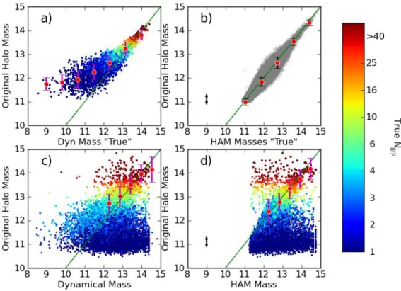
It is of interest to compare the dynamical masses to the HAM masses found for galaxy groups in the mock and in ECO catalogs. Because the HAM masses do not directly depend on the virialization state of the group, we would expect substantial scatter in the agreement between the two methods. We apply the methods described in §3.2 to both the mock catalog true groups and mock catalog FoF extracted groups. We compare all these mass mea-surements to original halo masses in Fig. 4. Here, all comparisons show only groups with Ngrp ≥ 3. Fig. 4a compares the dynamical masses of true groups to their true halo mass and shows a systematic underestimation in dynamical mass that increases in effect for groups with fewer members. To avoid this effect we restrict our later analysis that uses these estimations ofMdynfor ECO to groups withNgrp≥5. Panel b in Fig. 4 shows a similar comparison of true group HAM masses with their mock halo mass. This figure utilizes the entire simulation box. The scatter in this relationship comes from the
random-ness in the assignment of galaxy luminosities to groups based on their halo mass when defining the mock cat-alog (§2.2). We believe the tapering of the scatter for groups withMhalo<12.0 is due to the fact that random scatter was not added when populating halos with cen-tral galaxies, only satellites. The majority of these lower mass halos are isolated and contain only a central galaxy, so there is little luminosity scatter from populating these halos with satellite galaxies.
In addition to the scatter in Fig. 4b there is also a possible offset due to cosmic variance. The magnitude of this offset can be found using the results of Hu & Kravtsov (2003) who quantify the uncertainties due to cosmic variance and sample variance on perceived local cluster abundances (displayed in their Fig. 2). The re-lationship Hu & Kravtsov (2003) find can be scaled by RECO= 37 Mpc/h andh= 0.7 in order to find the pos-sible shift in the halo mass function that would affect the ECO sample and represent this shift by the black arrow in the bottom left corner of Fig. 4d. This shift in the halo mass function would translate to shifts in HAM masses. In Fig. 4b we see very little shift from the one-to-one line indicating the effects of cosmic variance are not significant for the mock catalog. Nevertheless, this shift could still be present in the ECO sample depending on the extent to which cosmic variance affects it.
In comparing galaxies’ halo masses with their dynami-cal masses or HAM masses determined for FoF extracted groups (Fig. 4c,d), we can see the effects of the group finder. There is a population of galaxies in Fig. 4c,d that have high dynamical masses, but low halo masses. These galaxies were originally isolated or living in very low mass halos but were linked to larger groups and therefore in-herited the larger halo mass. While a large number of these truly isolated galaxies are in the outskirts of their new groups, it is impossible to remove them using ob-servable parameters without also removing true group members. It will therefore be just as unclear in the real data to discern whether an object is a true group member or not. The D-S test can be used to identify subgroups that were a possible result of the group finder merging two groups, however this test will be unable to identify spatially scattered field galaxies on the edges of a group. Fortunately, these misgrouped field galaxies do not sig-nificantly affect the dynamical or HAM masses of the original group, since the groups that were originally in high mass halos remain very close to the 1:1 line after group finding despite contamination from interlopers.
Despite the tighter trend in HAM masses pre-group finding, it is important to remember that there are uncer-tainties in the mass function used to assign HAM masses due to the effects of cosmic variance and differences in true group abundances compared to what is accepted.. Additionally, these masses rely almost solely on luminos-ity, which relates to many of the group properties we later study in this paper. Therefore, in order to avoid in-troducing covariance between galaxy properties and es-timated group masses we use the dynamical masses in the analysis of ECO groups and their galaxy member properties.
dy-Figure 4. Mass comparisons for the mock catalog. (a) Original halo masses plotted against dynamical masses of true groups. (b) Original halo masses plotted against HAM masses of true groups and reflects the random scatter in group luminosities assigned at fixed mock halo
mass. The black arrow in the bottom left shows the possible shift due to cosmic variance in the halo mass function described in§4.2.
Note: this plot uses data from theentire simulation box. (c) Dynamical masses of FoF extracted groups compared to their original halo
masses. (d) HAM masses of FoF-extracted groups compared to original halo masses. The black arrow indicates the same possible offset due to cosmic variance as described for panel b. Each point is a galaxy, however if groups remain in their true halo after group finding then all galaxies in that group will be over-plotted on top of each other. Therefore, the scatter in the plot as an indication in the error on a single galaxy’s mass estimation is misleading because the density of points is not visualized. For all panels, only groups with FoF
extracted group numberNgal ≥3 are plotted. The color scale represents the number of members in each galaxy’s original ‘true group’,
where dark blue corresponds to galaxies that were originally isolated before group finding. One-to-one lines are plotted in each frame in
green and dispersion bars are shown in red, where the center is the median of that bin. In frames c and d bins are restricted toM >12 in
both the x and y axis to exclude the large population of dark blue outliers.
namical masses for the more massive groups (13 logM).
For smaller groups with 5 or fewer members, the trend switches and dynamical masses become higher. This in-dicates that the mass measurements for ECO groups are behaving in a similar way as they do in the mock catalog. The disagreement between methods is likely due to the fact that these methods are sensitive to different parame-ters. The dynamical mass method is much more sensitive to whether a system is virialized or not, while the HAM masses depend on luminosity of the group. Because of the sensitivity of the dynamical masses, they significantly underestimate small group (Ngrp <5) masses. While it may be tempting to use the comparison between these mass measurements in the mock to correct the underes-timation of the dynamical masses or the overesunderes-timation of the HAM masses, a large source of this difference is the results of the group finder. It is unclear whether the mock catalog’s definition of isolated galaxies is really true since it is not clear whether these galaxies might actu-ally be feeling the gravitational influence of the nearby group with which the group finder merges it. We can say however, that it is safe to trust the masses of high mass groups with N ≥ 5 members where the two methods roughly agree with the least scatter.
We additionally present the relationship between group mass and group size. Fig. 6 shows that this relationship follows a logarithmic trend in group number, with more scatter at lowNgrp. The color scale of Fig. 6 shows that HAM masses also produce the same trend. Groups with Ngrp > 20 correspond to halos of mass approximately greater than 1013.5 M.
4.3. Identifying Substructure
In order to gain more insight on group membership issues affecting group mass estimations, we apply the the Dressler-Schechtman (DS) test described in §3.3.2 to galaxy groups in ECO with the goal of identifying subgroup components. We also compare the results of this test with the Gaussianity of each group’s velocity distribution characterized by the Anderson-Darling test described in§3.3.1.
p-11.0 11.5 12.0 12.5 13.0 13.5 14.0 14.5 15.0 HAM Masses
9 10 11 12 13 14 15
Dynamical Masses
(a) ECO Catalog
3 Ngrp 5 Ngrp>5 α <5%
11 12 13 14 15
HAM Masses 9
10 11 12 13 14 15
Dynamical Mass
(b) Mock Catalog
3 Ngrp 5 Ngrp>5
Figure 5. Comparison of dynamical masses to HAM masses for FoF extracted groups in ECO and mock catalogs. (a) Group halo
mass methods compared for ECO groups with 3≤Ngrp≤5 shown
in pink and those in groups with Ngrp ≥ 5 shown in Carolina
blue. Groups with A-D classified non-Gaussian velocity dispersions (α <5%) are depicted as navy stars. (b) A similar comparison for mock catalog FoF extracted groups. Larger triangular symbols
represent groups with Ngrp ≥ 5 while smaller points represent
groups with 3≤Ngrp≤5. The color scale matches that of Fig. 4.
8 9 10 11 12 13 14 15
Dynamical Mass
10
010
110
210
3N
grp
ECO Groups
11.6
12.0
12.4
12.8
13.2
13.6
14.0
14.4
HAM Masses
Figure 6. Group number versus group dynamical mass is shown. Each group is also colored according to its group HAM mass. The
horizontal purple line is showing the dividing line atNgrp= 20.
values indicating the presence of substructure are shown. One group considered virialized as classified by both the A-D and D-S tests is also presented. Each galaxy is color coded by itsδvalue, which indicates how much the local velocity distribution deviates from the whole. Galaxies with similar δ values are not necessarily related, how-ever regions of nearby galaxies that all contain similar
δ values are. For the top three groups shown in Fig. 7 possible subgroups are selected based on their δ values (left panels) and the corresponding histograms of their velocity distributions are plotted (right panels). The red-der points indicate the largest deviations, while the bluer points show the smallest. Likewise, the red histograms that show the highδgalaxies have a very narrow range in velocities, while the blue histograms for the low-δ galax-ies cover a broader range of velocitgalax-ies, more closely re-sembling the overall velocity distribution for the groups (the purple histogram).
The groups shown in Fig. 7 are representative of the different types of interpretations that can be made based on velocity distributions. ECO group 4625 shows what could be a filament leading to a group. The filament (in blue) has a non-Gaussian velocity distribution, in con-trast to the more circularly shaped group. ECO group 806 shows what could be two subgroups connected by a central structure. ECO group 5410 shows less obvious segregation in comparison to the first two groups, per-haps because the group has begun to relax and the sub-groups components have begun mixing. These multiple-component groups will have overestimated dynamical masses due to larger measured radii and velocity disper-sions. There are many cases where there are no obvious subgroups as seen in these examples. However, if sub-groups were present and they were spatially overlapping and therefore appeared mixed, the D-S test would not be able to tell. In any case, this test serves as a power-ful tool for identifying structures found by FoF that are not virialized or are really composed of multiple compo-nents. Using the D-S test to identify interesting systems that are not virialized will be the subject of future work. In particular we would like to enhance this test by com-bining it with a center locating algorithm so subgroups can be systematically identified.
185.5 186.0 186.5 187.0 RA
45.0 45.2 45.4 45.6 45.8 46.0
46.2 p <10−4 α = 0.0025 M
halo=1013.5M¯
1.5 3.0 4.5 6.0 7.5 9.0 10.5
δ
0 2 4 6 8
Group 4625 , Ngrp = 23
0 2 4
6 δ <4.6
6600 6700 6800 6900 7000 7100 7200 7300 7400 Velocity (km/s)
0 2 4
6 δ >4.6
209.5 210.0 210.5 211.0 211.5 212.0 RA
9.0 9.5 10.0
DEC
p <10−4 α = 0.0001 M
halo=1014.5M¯
6 9 12 15 18 21 24 27
δ
0 3 6
9 Group 806 , Ngrp = 70
0 3 6
9 δ <10
0 3 6
9 10< δ <20
5000 5500 6000 6500 7000 7500
Velocity (km/s) 0
3 6
9 δ >20
188.4 188.6 188.8 189.0 189.2 RA
26.0 26.2 26.4 26.6 26.8 27.0 27.2 27.4
DEC
p <10−4 α = 0.0924 M
halo=1014.1M¯
5.0 7.5 10.0 12.5 15.0 17.5 20.0 22.5
δ
02 4 6
8 Group 5410 , Ngrp = 43
02 4 6
8 δ <8.5
02 4 6
8 8.5< δ <13.5
5800 6000 6200 6400 6600 6800 7000 7200 7400 7600 Velocity (km/s)
02 4 6
8 δ >13.5
202.4 202.6 202.8 203.0 203.2 203.4 203.6 RA
7.0 7.2 7.4 7.6 7.8 8.0
DEC
p= 0.17 α = 1.28 Mhalo=1013.6M¯
0.8 1.2 1.6 2.0 2.4 2.8 3.2 3.6 4.0
δ
6200 6400 6600 6800 7000 7200 7400
Velocity (km/s) 0
1 2 3 4 5 6 7 8
Group 3672 , Ngrp = 21
Figure 7. Three groups that show evidence of dynamical substructure and one that does not. Scatter plots of each galaxy’s coordinates
are shown on top, color coded by the deviation,δ, calculated for each galaxy according to Eq. 8. Symbol size is indicative of a galaxy’s
spatial distribution of galaxies in addition to their veloc-ities. Additional tests that work well for smaller groups (Ngrp <11) should also be explored that could help us gain a better picture of the virialization state of these smaller groups.
4.4. Environmental Effect on Galaxy Properties
Color and star formation are studied in ECO groups in order to understand environmental effects on selected galaxy properties. We use our group dynamical mass estimates to characterize environment and also restrict our analysis to galaxies falling within the virial radius as define in§3.2, unless otherwise noted.
4.4.1. Color
To study environmental effects on galaxy color, we first study the distribution of galaxies on the blue and red se-quences for systems of various sizes. The first analysis is displayed in Fig. 9, which shows the red and blue se-quences (divided by (u−r)e≈1.6, see Moffett et al., sub-mitted, for more accurate piece-wise division) in a plot of color versus stellar mass for ECO galaxies split into three subsets: field galaxies, groups with 3< Ngrp <20, and higher mass groups withNgrp >20. It is clear that the fraction of blue sequence galaxies decreases significantly between field galaxies and galaxies living in high mass groups. We find that 80% of field galaxies (Ngrp = 1) live on the blue sequence.
To study variations in galaxy color across group mass scales, the fraction of galaxies inside the virial radius that are on the red sequence of each ECO group is plot-ted against group dynamical mass in Fig. 10. There is a rough upward trend in the data indicating the presence of more red sequence galaxies dominating the popula-tion in higher mass halos. The transipopula-tion to becoming red-sequence dominated appears to be gradual. How-ever, forMhalo>13.5 the red-sequence fraction remains uniformly above 40%, which is more clearly shown by the red histogram in Fig. 11. A KS test proves this distribution is very different than that of the blue his-togram, which represents groups withMhalo<12.5, with a probability of being drawn from the same sample of 5×10⁻⁸. We can conclude there are a higher fraction of red-sequence galaxies in high mass halos and a higher fraction of blue-sequence galaxies in low mass halos. This result agrees with past studies such as that of Tanaka & Kodama (2004), who also find a higher fraction of red galaxies in group and cluster environments.
4.4.2. Gas Fraction
We also study the fraction of gas dominated galaxies as a function of halo mass for ECO+A groups (see§2.1). We defined gas dominated galaxies as having more HI mass than stellar mass and determine for each group the fraction of gas dominated galaxies within the virial ra-dius. The results are shown in Fig. 12 where each group is color coded by its α parameter from the A-D virial-ization test. While there is a smaller subset of points because ECO+A is about a third the size of ECO, there is still a clear drop in the data pastMdyn= 13.5 logM.
After this mass scale groups uniformly contain fewer than 25% gas dominated galaxies within their virial radius, with the exception of one outlier, ECO group 806 pre-sented in Fig. 7. This group is likely made of multiple
components that are individually less massive than cal-culated dynamically for the whole group. If this is true, components of ECO group 806 would shift left on the plot and more closely follow the trend.
In Fig. 12 there are several groups that have no gas dominated galaxies within rvir. These galaxies have α values lower than about 0.50, which is surprising because it is expected that lower gas content would associate with systems that are in a virialized state. However about 90% of these groups have 6 or fewer group members within their virial radii. The smaller number of group members makes theαmeasurement less robust and while the lack of gas dominated galaxies is significant, the small number of group members additionally makes it easier for the fraction to reach zero. No clear relation between αand fraction of gas dominated galaxies emerges, except for highly unvirialized (α <0.05) groups that tend to have a higher than average fraction of gas dominated galaxies. This trend supports the idea that unvirialized systems are less compact and less dense. Galaxies are still falling into these less dense systems and therefore these galaxies will be more capable of holding onto their gas.
4.4.3. Star Formation
To understand environmental effects on star formation activity, the median FSMGR (defined in§2.1) was found separately for galaxies inside and outside the virial ra-dius in each group and plotted versus halo mass (Fig. 13). For these groups, the median FSMGR is on aver-age higher in galaxies outside the virial radius than those withinrvir. This result is expected since processes such as ram pressure stripping and strangulation will occur first and more strongly for galaxies near the center of a group, where the density is higher than in the out-skirts. It is interesting however, that past the mass scale of 1013.5 M
, the median FSMGR of galaxies both
in-side and outin-side the virial radius for all groups (except one outlier that is ECO Group 806 shown in Fig. 7), remains below 0.5. Even in this outlier group, median FSMGR within the virial radius still follows the trend, though as discussed in§4.3 and Fig. 7, this group’s mass is likely actually composed of the mass of three unvirial-ized subgroups. The reduction in scatter in median FS-MGR past 1013.5 M
suggests a physical change in all
these groups causing a drastic, uniform decline in recent star formation. The mass scale of 1013.5Mhas come up
in other works including that of Robotham et al. (2006) who study galaxy luminosity functions (LF) for groups of varying group mass and find LF parameters stabilize starting at a mass of 1013.5M
, suggesting that at this
mass, processes such as quenching and merging are done occurring. This picture agrees with what is seen in Fig. 13, where a large fraction of groups below 1013.5M
have
large FSMGR and therefore have had recent star for-mation activity, inside and outside rvir, indicating that quenching processes have not yet suppressed all star for-mation.
0.0 0.5 1.0 1.5 2.0 alpha
0 5 10 15 20 25
11 Ngrp<25 5
10 15 20 25
delta
25 Ngrp<50 5
10 15 20 25
Ngrp≥50
ECO
0.0 0.5 1.0 1.5 2.0
alpha
05
1015
20 25 5
1015
20 25
delta
5
1015
20
25 MOCK
0.0 0.5 1.0 1.5 2.0
alpha 0
5 10 15 20 25 5 10 15 20 25
delta
5 10 15 20
25 MOCK (true)
Figure 8. Comparison of αand δ from the A-D and D-S tests, respectively. From left to right: ECO groups, mock catalog groups
post-FoF, mock catalog true groups. Groups with 10< Ngrp<25 are shown in blue, groups with 25≤Ngrp<50 are in yellow, and groups
withNgrp≥50 are in red. Each point is a galaxy. Highδvalues indicate large discrepancies between a galaxy’s local velocity distribution
and that of its groups. Large groupαindicates a Gaussian velocity distribution and largerδfor a galaxy indicates a more discrepant local
velocity distribution when compared to that of the whole group. Larger groups have lowerαand a higher maximumδvalue for both the
ECO and post-FoF mock catalogs, but the true mock catalog shows theα-dependence to be an artifact of group finding.
0.0 0.5 1.0 1.5 2.0 2.5
Field (
Ngrp= 1)
0.0 0.5 1.0 1.5 2.0 2.5
(
u
−
r
)
e
3 Ngroup 20
8.0 8.5 9.0 9.5 10.0 10.5 11.0 11.5
Stellar Mass 0.0
0.5 1.0 1.5 2.0 2.5
Ngroup>20
Figure 9. Extinction corrected color (u - r) versus stellar mass for field galaxies, galaxies in groups with fewer than 20 members, and
galaxies in large groups withNgrp>20. The relationship between
halo mass andNgrpis shown in Fig. 6.Ngrp= 20 corresponds to
roughly 1013.5 M
.
past the virial radius. The extent of environmental ef-fects past the virial radius has been seen in other studies including Bah´e et al. (2013). Future work could involve determining the radius at which environmental effects are no longer seen.
5. CONCLUSION
We have determined a robust method for measuring dynamical masses of galaxy groups through optimiza-tion on a mock catalog. By comparing dynamical masses found for FoF extracted groups to those found for origi-nal mock catalog groups, we determined that FoF linking lengths of bz = 0.12 and b⊥ = 1.3 reproduced the best
group masses relative to other tested linking lengths.
11.0 11.5 12.0 12.5 13.0 13.5 14.0 14.5 15.0
Group Dynamical Mass
0.0
0.2
0.4
0.6
0.8
1.0
Fraction of Galaxies on the Red Sequence
Inside
RvirFigure 10. Fraction of galaxies inside rvir that are on the red
sequence for ECO groups with Ngrp ≥ 5 plotted against group
mass. Bars show the dispersion in the red sequence fraction and are positioned at the median for that bin. A vertical line is drawn
atMhalo= 13.5 logMfor reference. The fraction of galaxies on
the red sequence for all isolated galaxies (not shown) is 20 %.
0.0Fraction of Galaxies on the Red Sequence0.2 0.4 0.6 0.8 1.0 0
10 20 30 40 50 60 70
Number of Groups
All Galaxies 11 < Mhalo < 12.5 12.5 < Mhalo < 13.5 Mhalo > 13.5
Figure 11. Histograms showing the distribution of the fraction of galaxies on the red sequence in ECO groups, plotted in Fig. 10. The gray histogram shows the total for all groups and the colored histograms are defined by different ranges in halo mass. Groups
withMdyn >1013.5 Mare uniformly composed of at least 40%
red-sequence galaxies.
11 12 13 14 15 Dynamical Mass
0.0 0.1 0.2 0.3 0.4 0.5 0.6
Fraction of Gas Dominated Galaxies
α <0.05
α >1.0
Figure 12. Fraction of gas dominated galaxies for ECO+A groups. A galaxy is considered gas dominated if it has an HI to stellar mass ratio greater than one. Groups that are considered
un-virialized (α < .05) are presented as black stars while groups with
very Gaussian velocity distributions (α >1.0) are shown as red
triangles. This analysis was performed using only galaxies within the virial radius of the group.
11.0 11.5 12.0 12.5 13.0 13.5 14.0 14.5 15.0Dynamical Mass of Group 0.0
0.5 1.0 1.5 2.0 2.5 3.0 3.5 4.0
Median FSMGR
r<rvir
11.0 11.5 12.0 12.5 13.0 13.5 14.0 14.5 15.0Dynamical Mass of Group 0.0
0.5 1.0 1.5 2.0 2.5 3.0 3.5 4.0
Median FSMGR
r>rvir
Figure 13. Median FSMGR for galaxies falling inside and outside
the virial radius of their group. A line at 1013.5M
points out
the apparent divide above which scatter in the median FSMGR of groups drops significantly. Galaxies in groups with mass greater
than 1013.5M
collectively show very low amounts of recent star
formation. Red circles points (top plot) and blue points (bottom plot) are found by taking the median FSMGR for galaxies inside
and outsidervir, respectively. Large blue and red points show the
median of the y-axis for separate dynamical mass bins and the corresponding bars represent the median absolute deviation in the data points for each bin.
are underestimated for groups with few members and we can only trust dynamical mass estimates for groups with Ngrp ≥ 5. We compare HAM masses to dynam-ical masses and find both mass estimates are affected
by faults in the group finding where originally isolated galaxies are merged onto larger groups. However, these additional ‘merged’ galaxies do not significantly alter the mass of the original massive group.
The optimized dynamical mass methods were applied to the ECO catalog, which contains about 340 groups with Ngrp ≥ 5. We compared dynamical mass mea-surements of ECO groups to corresponding HAM masses and found a similar trend as in the same comparison performed using mock catalog groups. At high masses, HAM masses slightly exceed dynamical masses, whereas the trend switches for Mhalo < 12.5 log M. We find
that in the mock catalog there are many galaxies that were originally isolated but were grouped onto larger groups and adopted the larger halo mass. This is psumably happening in ECO groups and therefore to re-duce this effect when studying galaxy properties we split up groups into two subsets composed of group members residing either inside or outside the virial radius of their group. We believe using a modified FoF group finding algorithm could help with contamination from merged groups or unassociated edge galaxies, however this task is difficult. Because unvirialized groups would result in larger dynamical masses than expected for relaxed sys-tems we use virialization tests to try to identify cases of unvirialization.
To assess the virialization state of ECO groups, two statistical methods, the A-D and D-S tests, were used that perform measures of group velocity distribution. The A-D test measures how Gaussian a group’s veloc-ity distribution is, while the D-S test returns a p-value that indicates how likely it is that a system contains sub-group components. We find that when a sub-group’sp-value indicates a high likelihood for the presence of substruc-ture, theαparameter given by the A-D test agrees and suggests a non-Gaussian velocity distribution. For the groups with obvious substructure, it is easy to separate the likely subgroups according to each galaxy’sδ value. However, a more robust method of identifying the mem-bers and spatial centers of these subgroups must still be developed. For groups whose virialization state is un-clear, the two statistics did not always agree. The D-S test could only be used on groups with more than 10 members and most groups with substructure according to theirp-value were also among the highest mass groups. This relation seems to arise partly due to the nature of the test, but also in part due to the group finder, which increases the amount of contamination from interlopers and causes these groups to appear less virialized. For smaller groups it is also more possible for a fraction of a galaxy’s ten nearest neighbors to not all be related, therefore making it more difficult to identify substruc-ture around that galaxy. While the D-S test identified groups with interesting internal dynamics, different tests for deducing the virialization state of groups of all sizes are desired. More analysis of the A-D test that judges the Gaussianity of a group’s velocity dispersion are needed, in addition to incorporating tests that utilize the pro-jected spatial positioning of group members.
a larger fraction of more massive galaxy groups. There is also a transitional mass scale at 1013.5M
above which
group median FSMGR remains below 0.5 for all groups, indicating quenching processes have fully suppressed star formation in these massive systems. In future work, we wish to study these group properties as a function of ra-dius from the group center.
6. ACKNOWLEDGEMENTS
I would like to thank my very supportive and help-ful advisor Sheila Kannappan, as well as my summer research advisor Andreas Berlind for the many discus-sions about and help with the theoretical aspects of this project. Also many thanks to Amanda Moffett for mak-ing the ECO catalog and for her continued help. We acknowledge NSF funding support to Vanderbilt under REU grant PHY-1263045 and to the RESOLVE survey at UNC Chapel Hill under AST-0955368.
REFERENCES
Applegate, D. E., von der Linden, A., Kelly, P. L., et al. 2014, MNRAS, 439, 48
Bah´e, Y. M., McCarthy, I. G., Balogh, M. L., & Font, A. S. 2013,
MNRAS, 430, 3017
Balogh, M. L., Navarro, J. F., & Morris, S. L. 2000, ApJ, 540, 113 Becker, M. R., & Kravtsov, A. V. 2011, ApJ, 740, 25
Bekki, K. 1998, A&A, 334, 814
Bennett, C. L., Larson, D., Weiland, J. L., et al. 2013, ApJS, 208, 20
Berlind, A. A., Frieman, J., Weinberg, D. H., et al. 2006, ApJS, 167, 1
Blanton, M. R., & Berlind, A. A. 2007, ApJ, 664, 791 Cacciato, M., van den Bosch, F. C., More, S., et al. 2009,
MNRAS, 394, 929
Carollo, C. M., Cibinel, A., Lilly, S. J., et al. 2013, ApJ, 776, 71 Cohen, S. A., Hickox, R. C., Wegner, G. A., Einasto, M., &
Vennik, J. 2014, ArXiv e-prints, arXiv:1401.6171
Colless, M., Dalton, G., Maddox, S., et al. 2001, MNRAS, 328, 1039
D’Agostino, R. 1986, Goodness-of-Fit-Techniques, Vol. 68 Davis, M., & Djorgovski, S. 1985, ApJ, 299, 15
Dressler, A., & Shectman, S. A. 1988, AJ, 95, 985
Dressler, A., Oemler, Jr., A., Couch, W. J., et al. 1997, ApJ, 490, 577
Driver, S. P., Hill, D. T., Kelvin, L. S., et al. 2011, MNRAS, 413, 971
Duarte, M., & Mamon, G. A. 2014, ArXiv e-prints, arXiv:1401.0662
Evrard, A. E. 1987, ApJ, 316, 36
Falco, E. E., Kurtz, M. J., Geller, M. J., et al. 1999, PASP, 111, 438
Giovanelli, R., & Haynes, M. P. 1985, ApJ, 292, 404 Girardi, M., Giuricin, G., Mardirossian, F., Mezzetti, M., &
Boschin, W. 1998, ApJ, 505, 74
Gunn, J. E., & Gott, III, J. R. 1972, ApJ, 176, 1
Haynes, M. P., & ALFALFA Team. 2008, in American Institute of Physics Conference Series, Vol. 1035, The Evolution of Galaxies Through the Neutral Hydrogen Window, ed. R. Minchin & E. Momjian, 238–241
Holmberg, E. 1941, ApJ, 94, 385
Hou, A., Parker, L. C., Harris, W. E., & Wilman, D. J. 2009, ApJ, 702, 1199
Hu, W., & Kravtsov, A. V. 2003, ApJ, 584, 702 Huchra, J. P., & Geller, M. J. 1982, ApJ, 257, 423
Jauzac, M., Jullo, E., Kneib, J.-P., et al. 2012, MNRAS, 426, 3369 Jones, D. H., Read, M. A., Saunders, W., et al. 2009, MNRAS,
399, 683
Kannappan, S. J., Stark, D. V., Eckert, K. D., et al. 2013, ApJ, 777, 42
Kawata, D., & Mulchaey, J. S. 2008, ApJ, 672, L103 Lacey, C., & Cole, S. 1994, MNRAS, 271, 676
Larson, R. B., Tinsley, B. M., & Caldwell, C. N. 1980, ApJ, 237, 692
Li, I.-H. 2007, PhD thesis, University of Toronto, Canada Li, I. H., & Yee, H. K. C. 2008, AJ, 135, 809
Moffett, A., Kannappan, S., Berlind, A., et al. sumbitted Nelson, L. 1998, Journal of Quality Technology, 30, 298 Nulsen, P. E. J. 1982, MNRAS, 198, 1007
Paturel, G., Theureau, G., Bottinelli, L., et al. 2003, A&A, 412, 57
Press, W. H., & Schechter, P. 1974, ApJ, 187, 425
Quilis, V., Moore, B., & Bower, R. 2000, Science, 288, 1617 Rasmussen, J., Ponman, T. J., Verdes-Montenegro, L., Yun,
M. S., & Borthakur, S. 2008, MNRAS, 388, 1245
Robotham, A., Wallace, C., Phillipps, S., & De Propris, R. 2006, ApJ, 652, 1077
Takey, A., Schwope, A., & Lamer, G. 2011, A&A, 534, A120 Tanaka, M., & Kodama, T. 2004, in Baryons in Dark Matter
Halos, ed. R. Dettmar, U. Klein, & P. Salucci
Tempel, E., Tamm, A., Gramann, M., et al. 2014, ArXiv e-prints, arXiv:1402.1350
Warren, M. S., Abazajian, K., Holz, D. E., & Teodoro, L. 2006, ApJ, 646, 881
Weinmann, S. M., van den Bosch, F. C., & Pasquali, A. 2011, The Dependence of Low Redshift Galaxy Properties on Environment, ed. I. Ferreras & A. Pasquali, 29
Weinmann, S. M., van den Bosch, F. C., Yang, X., et al. 2006, MNRAS, 372, 1161
Wetzel, A. R., Tinker, J. L., & Conroy, C. 2012, MNRAS, 424, 232
Wetzel, A. R., Tinker, J. L., Conroy, C., & van den Bosch, F. C. 2013, ArXiv e-prints, arXiv:1303.7231
York, D. G., Adelman, J., Anderson, Jr., J. E., et al. 2000, AJ, 120, 1579