Efficient geometric sound propagation using visibility culling

(1)

Efficient Geometric Sound Propagation Using

Visibility Culling

Anish Chandak

A dissertation submitted to the faculty of the University of North Carolina at Chapel Hill in partial fulfillment of the requirements for the degree of Doctor of Philosophy in the Department of Computer Science.

Chapel Hill 2011

Approved by:

Dinesh Manocha

Gary Bishop

Ming C. Lin

Sorin Mitran

(2)

(3)

Abstract

Anish Chandak: Efficient Geometric Sound Propagation Using Visibility Culling.

(Under the direction of Dinesh Manocha.)

Simulating propagation of sound can improve the sense of realism in interactive

appli-cations such as video games and can lead to better designs in engineering appliappli-cations such

as architectural acoustics. In this thesis, we present geometric sound propagation techniques

which are faster than prior methods and map well to upcoming parallel multi-core CPUs. We

model specular reflections by using the image-source method and model finite-edge diffraction

by using the well-known Biot-Tolstoy-Medwin (BTM) model. We accelerate the computation

of specular reflections by applying novel visibility algorithms, FastV and AD-Frustum, which

compute visibility from a point. We accelerate finite-edge diffraction modeling by applying a

novel visibility algorithm which computes visibility from a region.

Our visibility algorithms are based on frustum tracing and exploit recent advances in fast

ray-hierarchy intersections, data-parallel computations, and scalable, multi-core algorithms.

The AD-Frustum algorithm adapts its computation to the scene complexity and allows small

errors in computing specular reflection paths for higher computational efficiency. FastV and our

visibility algorithm from a region are general, object-space, conservative visibility algorithms

that together significantly reduce the number of image sources compared to other techniques

while preserving the same accuracy. Our geometric propagation algorithms are an order of

magnitude faster than prior approaches for modeling specular reflections and two to ten times

faster for modeling finite-edge diffraction. Our algorithms are interactive, scale almost linearly

on multi-core CPUs, and can handle large, complex, and dynamic scenes. We also compare

the accuracy of our sound propagation algorithms with other methods.

Once sound propagation is performed, it is desirable to listen to the propagated sound in

interactive and engineering applications. We can generate smooth, artifact-free output audio

(4)

audio-processing algorithm for scenarios with simultaneously moving source and moving

re-ceiver (MS-MR) which incurs less than 25% overhead compared to static source and moving

(5)

(6)

Acknowledgments

The past five years as a graduate student in the Department of Computer Science at

UNC-Chapel Hill have been very rewarding, personally and professionally. I would like to thank

many people who have been an important part of my journey through these times. First and

foremost, I would like to thank my advisor Prof. Dinesh Manocha for his encouragement,

guidance, and support over the past five years. I am grateful for the freedom he gave me to

work on challenging research projects. I would also like to thank my committee members:

Prof. Ming C. Lin, for her guidance and generously sponsoring lunches and dinners during

paper deadlines; Prof. Gary Bishop for his insightful comments on my research and passionate

discussions on many other applications related to sound; Prof. Sorin Mitran for educating me

about numerical methods and other technical discussions; and Prof. Marc Niethammer for his

feedback and insightful comments on my thesis.

I have had the privilege to work with some really smart collaborators on various research

projects. I would like to thank them for teaching me so much and being patient with me.

In particular, I would like to thank Christian Lauterbach, Nikunj Raghuvanshi, Micah

Tay-lor, Zhimin Ren, Lakulish Antani, and Ravish Mehra. I would also like to thank members

of GAMMA group for their support and feedback. I would like to thank support staff at

the Department of Computer Science at UNC-Chapel Hill for their excellent assistance. In

particular, I would like to thanks Missy Wood, Janet Jones, Kelli Gaskill, and Mike Stone.

I would like to thank many good friends for making the past five years in Chapel Hill a

lot of fun. In particular, Sasa Junuzovic, Liangjun Zhang, Jason Sewall, Rahul Narain, Sachin

Patil, Vishal Verma, Lei Wei, and Qi Mo. I would like to especially thank my dear friends,

the Taylors (Micah, Christine, and Charlotte). Lastly, I would like to thank my parents,

Shyam and Vijaylaxmi Chandak, my brother and sister-in-law, Manish and Shital Chandak,

my sister, Surbhi Maheshwari, and my nephew and niece, Divit and Ananya Chandak, for

(7)

List of Figures

1.1 Sound rendering in video games . . . 3

1.2 Sound rendering in virtual reality (VR) applications . . . 6

1.3 Sound rendering in other applications . . . 7

1.4 Input modeling for sound rendering . . . 8

1.5 Example of sound propagation . . . 9

1.6 Overall sound rendering system . . . 18

2.1 Object-space exact visibility algorithms . . . 27

2.2 View-frustum culling and back-face culling . . . 30

2.3 Object-space conservative visibility algorithms . . . 31

2.4 Special scenes used for visibility computation . . . 32

2.5 Image-space visibility algorithms . . . 34

2.6 Overview of image source method . . . 40

2.7 Bell lab box validation [Tsingos et al., 2002] . . . 53

3.1 Accelerating the image-source method by using from-point visibility . . . 55

3.2 Overview of AD-Frustum technique . . . 56

3.3 AD-Frustum representation . . . 58

3.4 Visibility computation based on area subdivision . . . 59

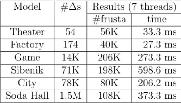
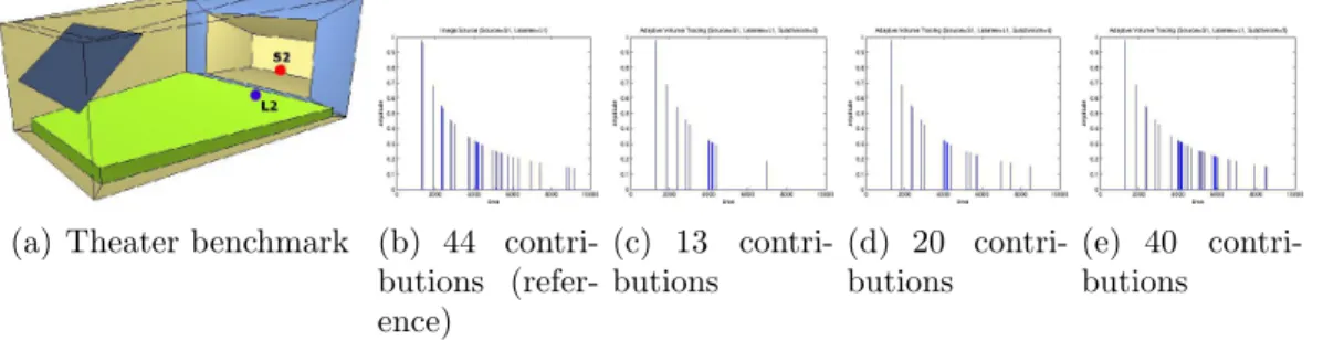
3.5 Benchmarks for AD-Frustum technique . . . 63

3.6 AD-Frustum: Effect of sub-division depth on performance . . . 63

3.7 Multi-core scaling of AD-Frustum . . . 64

(13)

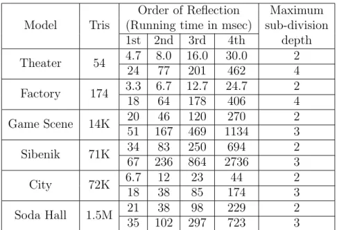
3.9 Shoebox validation: Configuration 1 . . . 70

3.10 Shoebox validation: Configuration 2 . . . 71

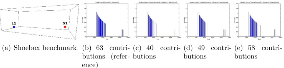
3.11 Theater validation: Configuration 1 . . . 71

3.12 Theater validation: Configuration 2 . . . 72

3.13 Dome validation: Configuration 1 . . . 72

3.14 Dome validation: Configuration 2 . . . 73

3.15 Factory validation: Configuration 1 . . . 73

3.16 Overview of FastV algorithm . . . 76

3.17 Frustum blocker computation . . . 78

3.18 Conservative Pl¨ucker tests . . . 80

3.19 Updating far plane depth . . . 81

3.20 Performance scaling vs. #Cores . . . 83

3.21 PVS Size vs. Ray Sampling . . . 85

3.22 Benchmarks for FastV . . . 87

3.23 PVS ratio vs. #Frusta . . . 87

3.24 FastV vs. Beam Tracing . . . 88

3.25 Ten key frames used for comparing the from-point PVS . . . 89

3.26 Convergence of FastV . . . 90

3.27 Occluder fusion . . . 92

3.28 Benchmarks for specular reflection modeling using FastV . . . 94

3.29 Geometric sound propagation approaches . . . 95

4.1 Overview of our conservative from-region visibility approach . . . 97

4.2 Frustum construction performed by FastV . . . 100

(14)

4.4 Occluder selection in 2D . . . 102

4.5 Accuracy issues with using from-point algorithms with separating frusta . 103 4.6 Benchmarks for from-region visibility . . . 105

4.7 An example of a visibility tree . . . 108

4.8 Overview of our image source method . . . 110

4.9 Image source of a diffracting edge . . . 112

4.10 Image sources for two successive diffractions . . . 113

4.11 Image sources for one diffraction followed by one specular reflection . . . 113

4.12 Diffraction paths between source S and listener Lacross edge E . . . 114

4.13 Second order diffraction paths between source S and listenerL . . . 114

4.14 Path validation for specular reflection and diffraction . . . 115

4.15 Benchmarks for accelerated images source method . . . 119

4.16 Some examples of diffraction paths computed by our algorithm . . . 120

4.17 Visible geometry comparison. . . 122

4.18 Accuracy of impulse responses computed by our system . . . 123

5.1 Integration of audio processing with sound propagation . . . 128

5.2 Example of a typical IR . . . 130

5.3 IR convolution . . . 131

5.4 Extrapolating the IR to estimate late reverberation . . . 133

5.5 Interpolation schemes applied for attenuation interpolation . . . 135

5.6 Fractional delay filter to obtain Doppler effect . . . 137

5.7 Sound propagation for MS-MR scenarios . . . 138

5.8 Audio processing pipeline for MS-MR scenarios. . . 138

(15)

5.10 Our modified image-source method for MS-MR . . . 145

5.11 Our modified Direct-to-Indirect Acoustic Radiance Transfer method . . . 146

6.1 Experimental setup . . . 150

6.2 Results for sourceS1 . . . 152

6.3 Spectrogram results for source S1 . . . 153

(16)

List of Tables

2.1 Visibility techniques . . . 36

2.2 Sound propagation techniques . . . 47

3.1 Adaptive Frustum Tracing vs. Uniform Frustum Tracing . . . 64

3.2 AD-Frustum sound propagation performance . . . 65

3.3 AD-Frustum performance for different sub-division depths . . . 66

3.4 FastV performance results . . . 86

3.5 Difference in the PVS computed by FastV and a beam tracer . . . 88

3.6 Acceleration for specular reflection due to using from-point visibility . . . 94

4.1 Performance of our occluder selection algorithm . . . 106

4.2 Benefit of our occluder selection algorithm . . . 106

4.3 Performance of individual steps of our algorithm . . . 119

4.4 Advantage of using visibility for second order edge diffraction . . . 121

5.1 Timing performance for late reverberation estimation . . . 134

5.2 Notation table . . . 139

5.3 Timing results for audio processing based on STFT . . . 143

5.4 MS-MR overhead for image-source method . . . 148

5.5 MS-MR overhead for D2I method . . . 148

6.1 Locations of the sound sources and the receivers . . . 150

6.2 Relative magnitude error (in decibel) for S1 . . . 158

6.3 Relative magnitude error (in decibel) for S2 . . . 158

(17)

Chapter 1 Introduction

Over the last few decades, the fidelity of visual rendering in interactive applications such as video games, virtual reality (VR) training, scientific visualization, and computer-aided design (CAD) has improved considerably [Tatarchuk, 2009]. The availability of high performance, low-cost commodity graphics processors (GPUs) makes it possible to render complex scenes at interactive rates on current laptops and desktops. However, in order to improve the immersive experience and utility of interactive applications, it is also important to develop interactive technologies that exploit other senses, especially the sense of hearing [Anderson and Casey, 1997].

(18)

definition of sound rendering as only recently has there been an active interest in these algorithms for interactive applications [Manocha et al., 2009]. There is a term often used in architectural acoustics similar to sound rendering; Auralization. Auralizationis the process of rendering audible, by physical or mathematical modeling, the sound field of a source in a space, in such a way as to simulate the binaural listening experience at a given position in the modeled space [Kleiner et al., 1993]. Auralization insists simulat-ing binaural listensimulat-ing experience and does not incorporate sound synthesis techniques. Further, given the recent trend towards highly parallel multi-core CPUs and many core GPUs it is possible to implement efficient algorithms for sound rendering.

In this chapter, we give examples of different applications of sound rendering, an overview of our problem statement, and a brief overview of prior approaches. Next, we discuss various issues and challenges in designing efficient techniques for sound propa-gation and audio processing as well as the main contributions of the thesis.

1.1 Applications

There are many applications that could benefit from sound rendering, especially sound propagation and audio processing. In this section, we give a brief overview of some of these applications. The challenges imposed by these applications on sound rendering algorithms are discussed in Section 1.4.

Video Games

(19)

Shad-(a) (b) (c)

Figure 1.1: Sound rendering in video games. (a) Stealth Games: In stealth games, the player must avoid detection and use stealth to evade or ambush antagonists. Thief: Deadly Shadows [EIDOS, 2011] is a popular stealth game where protagonist and mas-ter thief Garrett aims to steal his way through the City using stealth. Modeling sound propagation can help Garrett, the master thief evade the antagonists by using reflected and diffracted sound to detect their approach. (b) Multiplayer Games: Voice chat is an integral part of multiplayer games like Counter Strike [CSS, 2011]. It allows players on the same team to talk to each other, plan their strategies, and gain strategic advantage. Modeling the environment and position of the players during the voice chat can improve the overall realism and experience. Dolby recently released Axon [AXON, 2011], a voice chat middleware which modifies the voice chat between two players by taking into account reflection and diffraction of sound between the players. (c) First Person Shooter Games: First person shooter games, like Call of Duty [COD, 2011], are a very popular genre of games where the player experiences the action through the eyes of the protagonist. In first person shooter games sound rendering can help the player to detect the enemies, improve realism, and enhance the overall gaming experience of the players.

(20)

Currently, video games use simple sound propagation models. In most games only the direct sound from a source to a receiver is modeled. Occlusion, diffraction, and reflection of sound are approximated by applying artist created filters [Kastbauer, 2010]. These filters are created manually by artists, instead by using a sound propagation simulation. For example, to model echoes in a cathedral, artists may use a filter which sounds like a cathedral, but only a single filter is created for the whole space and it does not vary with relative positions of the sound source and the receiver. There are many reasons for these limitations. Firstly, interactive performance is required in video games and typically only a fraction (<10%) of the total CPU budget is devoted to sound rendering. Thus, interactive sound rendering algorithms which stay within the allotted CPU budget need to be developed. Secondly, video games typically use geometric models ranging from small rooms to big cities consisting of tens to a few hundreds of thousands of triangles. Such complex models are challenging to handle efficiently for current sound rendering algorithms [Funkhouser et al., 2003]. Thirdly, the sound sources, receiver, and geometric objects in games can move, i.e. they are dynamic. Thus, sound rendering algorithms need to efficiently handle complex, dynamic, and general scenes. Further, it might be acceptable to trade-off accuracy for higher computational performance in video games.

Virtual Reality Training

(21)

or set the mood [Mann, 2008]. For example, reverberation provides a sense of warmth or immersion in the environment. An example of a VR simulator, where sound ren-dering can significantly improve its effectiveness, is one used for treating soldiers suf-fering from post-traumatic stress disorder (PTSD) [Wilson, 2010] (see Figure 1.2(a)). An accurate reproduction of the sound field is important to recreate a believable war experience in the training environment so that the soldiers suffering from PTSD can ex-perience the intense war-like environment in a controlled setting [Hughes et al., 2006]. Other VR simulators where sound rendering could significantly improve their utility are combat training simulators like, the Future Immersive Training Environment (FITE) [Pellerin, 2011], and training simulators for the visually impaired, like the HOMERE system [Lecuyer et al., 2003, Torres-Gil et al., 2010]. These VR simulators can be sig-nificantly enhanced by incorporating advanced sound rendering techniques.

Like games, VR training simulators require interactive sound propagation. Also, the output audio should have minimal artifacts due to dynamic sources, receiver, and scene geometry. However, the typical resource limitations of games can be ignored and more computational resources can be devoted to sound rendering in these applications. Accurate sound rendering may be required as it is important to faithfully reproduce the sounds in the VR environment.

Architectural Acoustics

(22)

(a) (b) (c)

Figure 1.2: Sound rendering in virtual reality (VR) applications. (a) Therapy Systems: U.S. Air Force Senior Airman Joseph Vargas, uses the Virtual Iraq program at Mal-colm Grow Medical Center’s Virtually Better training site at Andrews Air Force Base, Md., June 25, 2009. The 79th Medical Wing is one of eight wings that uses this new technology to treat patients suffering from post-traumatic stress disorder (PTSD). U.S. Air Force photo by SRA Renae Kleckner [Wilson, 2010]. Recreating a realistic war ex-perience for a patient is critical for such applications to be useful for PTSD treatment. An accurate and efficient modeling of the sound field during a virtual war simulation increases the presence of the patient in the virtual war simulation [Hughes et al., 2006] and hence, significantly improves the technology to treat PTSD patients. (b) Combat Training Systems: US Marines walk through a Future Immersive Training Environment (FITE) scenario. This Defense Department program provides 3D immersive technolo-gies to help Marines and soldiers make better, faster decisions on the ground. Sound rendering can improve the system by providing sound cues which are an integral part of the decision making process on the ground. (c) Training Systems for the Visually Im-paired: HOMERE system: a multimodal system for visually impaired people to explore and navigate inside virtual environments. It has an auditory feedback for the ambient atmosphere and for other specific events. Sound rendering can significantly improve such a system by providing auditory feedback as the sound bounces around in the virtual environment.

(23)

(a) (b) (c)

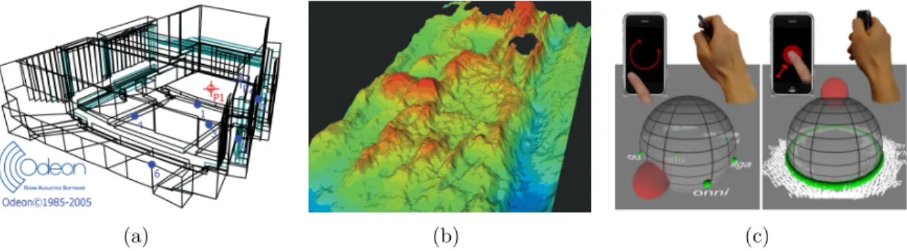
Figure 1.3: Sound rendering in other applications. (a) Architectural Acoustics: Acoustic modeling is the prediction of the sound field in a particular 3D design of a building, e.g. concert halls, offices, and class rooms. The clarity of speech is very important in class rooms for students to be able to listen and understand the lectures. Likewise, the rever-beration of music in concert halls is important for a great listening experience. Standard guidelines for acoustics in such spaces has been defined [ANSI/ASA S12.60-2002, 2002]. ODEON is a popular acoustic modeling software [Christensen, 2009]. Sound render-ing can model and correct the acoustics durrender-ing the design phase and could help save cost by preventing expensive post-construction fixes. (b) Multimodal Scientific Visu-alization: A display of bathymetric data using three dimensions and color; additional data is provided by generating forces and sounds as a user explores the surface with a haptic display device. (Figure courtesy NASA/UH Virtual Environments Research Institute.) (c) Auditory Interfaces: A method for browsing eyes-free auditory menus [Kajastila and Lokki, 2010]. Auditory menus are spoken one by one; the user has the ability to jump to the next item and to stop the current playback.

e.g. architectural models represented as cells and portals, 2.5D urban models, or scenes with large convex primitives. Further, prior acoustics modeling tools do not exploit commodity processors in terms of multiple cores.

Multimodal Scientific Visualization and Auditory Interfaces

(24)

(a) (b) (c)

Figure 1.4: Input modeling for sound rendering. (a) Highly detailed CAD model for graphics modeling (left) and simplified CAD model for geometric acoustic modeling (right) [Vorl¨ander, 2008]. (b) A transfer function computed for a detailed object to encode scattering due to the object. The object can be replaced with a simpler object and a transfer function [Tsingos et al., 2007]. (c) Modeling of sound synthesis and radiation pattern due to a sound source [James et al., 2006].

low-pitch, bass type instrument, and long duration is used. And for high data values, a combination of high pitch, soprano type instrument, and a short duration is used. Some training may be required for a user to be able to associate a data value to the audio output from the multimodal visualization system [Loftin, 2003]. Auditory interfaces use audio as a key component to design better user interfaces. Figure 1.3(c) show an example of an eye-free method for accessingauditory menus [Kajastila and Lokki, 2010]. Auditory displays can augment graphical displays and provide the user with an enhanced sense of presence. Efficient sound rendering tools can be used to develop interesting multimodal visualization techniques and auditory interfaces.

1.2 Sound Rendering

In this section we review different components of sound rendering and prior state-of-the art in sound rendering.

1.2.1 Input Modeling

(25)

a receiver; and input geometric models with their acoustic material properties. Sig-nificant work has been done in the past few years on interactive modeling of sound source vibrations [Raghuvanshi and Lin, 2006], and modeling their transfer functions [James et al., 2006] (see Figure 1.4(c)). They are collectively studied under sound syn-thesis techniques. Many sound rendering systems focussing on sound propagation as-sume that the sound source is a point source with a uniform radiation pattern. The input audio to the source is anechoically recorded audio samples. In terms of a receiver, a point receiver with a transfer function, specifically a generalized Head Related Trans-fer Function (HRTF) [Algazi et al., 2001], which models the scattering of sound due to receivers’ head, torso, and shoulders has been used. This allows modeling of binaural audio, i.e. audio for left and right ear, at the receiver.

The CAD model and acoustic material properties are also provided as input by the sound rendering application. Many applications like video games use complex geometric models for visual rendering and the same model is provided as an input for sound rendering. 3D models with only relevant geometric details [Vorl¨ander, 2008] are needed by the sound rendering systems (see Figure 1.4(a)). However, very limited work has been done to automatically simplify a complex model for visual rendering to a simplified model for sound rendering [Siltanen et al., 2008]. Further, the acoustic material properties also need to be specified along with acoustic geometry. Recently, complex transfer functions [Tsingos et al., 2007] (see Figure 1.4(b)) similar to those used in computer graphics have been proposed for sound rendering. However, limited data is available on acoustic transfer functions of acoustic materials and simplified models.

1.2.2 Sound Propagation

(26)

ac-(a) (b)

Figure 1.5: Example of sound propagation. (a) Input scene with a point source (S) and a point receiver (R) and input scene model. Example of specular reflection, diffuse reflections, and diffraction from source to the receiver. (b) Propagation of sound in a constant linear medium can be characterized by computing response at the receiver due to an impulse sound emitted at the source, called impulse response (IR).

curately model sound propagation in a scene. However, despite recent advances in nu-merical methods to solve the acoustic propagation equation [Raghuvanshi et al., 2009], these methods can take hours to days to solve the wave equation and can be too slow for interactive applications. Further, they are restricted to modeling only low frequencies of sound waves as the computational overhead of numerical methods increase propor-tional to f4_{, where} _f _{is the maximum frequency modeled by the numerical methods}

[Botteldooren, 1995].

Most sound propagation techniques used in practical applications model the acous-tic effects of an environment using linearly propagating rays. Thesegeometric acoustics

(GA) techniques are not as accurate as numerical methods in terms of solving the wave equation, and cannot easily model all kinds of propagation effects, but they can simulate early specular reflections at real-time rates [Funkhouser et al., 2003]. They provide ap-proximate solutions to the wave equation for high-frequency sound sources. Figure 1.5(a) shows example of specular reflection, diffuse reflections, and edge diffraction using rays from a source to a receiver. Broadly, geometric acoustics algorithms can be divided into

pressure-based and energy-based methods.

(27)

acous-tic rendering equation [Siltanen et al., 2007] is an integral equation which generalizes many existing energy-based geometric techniques. Existing energy-based methods in-clude: ray tracing [Krokstad et al., 1968], phonon tracing [Kapralos, 2006], and radiosity [Nosal et al., 2004].

Pressure-based methods model specular reflections and edge diffraction, and are essentially variations of the image-source method [Allen and Berkley, 1979]. Ray tracing [Vorl¨ander, 1989], beam tracing [Funkhouser et al., 2004], and several other techniques [Funkhouser et al., 2003] have been proposed to accelerate the image-source method for specular reflections. Edge diffraction is modeled by the Uniform Theory of Diffraction (UTD) [Kouyoumjian and Pathak, 1974] or the Biot-Tolstoy-Medwin (BTM) model of diffraction [Medwin et al., 1982]. Propagation of sound in a constant linear medium can be characterized by computing the response at the receiver due to an impulse sound emitted at the source, called impulse response (IR). In image source method, and IR is computed from a collection of image sources by taking into account their position and direction relative to the receiver.

Image Source Method and Visibility Tree

The image source method [Allen and Berkley, 1979] is widely used for modeling specular reflections and has been extended to model finite-edge diffraction [Pulkki et al., 2002]. Given a point sourceSand a listenerL, it is easy to check if a direct path exists fromSto

L. This is a ray shooting problem. The basic idea behind the image source method is as follows. For a specular reflector (in our case, a triangle) T, a specular pathS →T →L

exists if the triangle T is visible from the source S and the listener L is visible from the

image ofS, created by reflectingSacross the plane of triangle T, through triangleT. In the absence of any visibility information, image sources need to be computed for every

(28)

the number of reflections. The image sources for a sound source computed this way can be encoded in a data structure called visibility tree.

For a given source position, this process can be accelerated as follows. Note that first-order image sources only need to be computed for triangles visible to S. For a first-order image source S1, second-order image sources only need to be computed for

the triangles that are visible toS1 through T, and so on for higher order image sources.

The same principle applies to finite-edge diffraction. The image source of a diffracting edge is the edge itself and higher order diffraction need to be computed for the edges that are visible to the diffracting edge. Thus, to accelerate the image source method, the goal should be to never compute image sources that do not contribute towards the IRs computed at the listener positions.

1.2.3 Audio Processing

In the audio processing step, we take the input audio played at the source and convolve it with the impulse responses (IRs), computed by the sound propagation step, to generate the output audio. To generate audio output for a left and right ear, i.e. binaural audio output, a transfer function is applied to each geometric path reaching the receiver. The transfer function could be a simple parametric left-right panning or more accurate head related transfer function (HRTF) computed by either measurements [Algazi et al., 2001] or physical simulation [Dellepiane et al., 2008] which takes scattering of sound due to the human head, torso, and shoulder into account.

(29)

au-dio processing low, efficient techniques based on perceptual optimization are required [Tsingos et al., 2004, Tsingos, 2005]. Additional challenges arise when both the sound source and the receiver are moving simultaneously as for a given receiver position, sound reaches the receiver form different source positions and very limited work has been done to address this issue. We will present a technique to address this issue in Chapter 5.

1.3 Visibility Techniques

Visibility computation is one of the classical problems that has been studied extensively due to its importance in many fields such as computer graphics, computational geometry, and robotics. Given a scene, the goal is to compute a potentially visible set (PVS) of primitives that are visible from a single point (i.e. from-point visibility), or from any point within a given region (i.e. from-region visibility). Visibility algorithms can be classified in different ways. One way is to classify them into point and from-region visibility. From-point visibility is used in computer graphics for generating the final image from the eye-point based on rasterization [Theoharis et al., 2001] or ray tracing [Arvo and Kirk, 1989]. Other examples of applications of from-point visibility include hard shadow computation for point light sources. From-region visibility has been used in computer graphics for global illumination (i.e., computing the multiple bounce response of light from light sources to the camera via reflections from primitives in the 3D model), interactive walkthroughs of complex 3D models by pre-fetching a smaller set of potentially visible primitives from a region around the active camera position, soft shadow computation from area light sources, etc.

1.3.1 Object-Space Exact Visibility

(30)

algo-rithm is the smallest PVS which contains all the primitives. These technique per-form intersection computations at the accuracy of the original model, e.g. IEEE 64-bit double precision arithmetic. Many applications require exact visibility with object-space precision. For example, accurate computation of soft shadows due to area light source in computer graphics [Hasenfratz et al., 2003] requires the computation of ex-act visible area from all the points of the area light source to compute the contri-bution of the area light source at the point. Similarly, computing hard shadows due to a point light source requires accurate computation of visible portions of primitives from the point light source [Lloyd et al., 2006] or aliasing artifacts may appear. Many approaches have been proposed for exact from-point [Heckbert and Hanrahan, 1984, Overbeck et al., 2007, Nirenstein, 2003] and from-region visibility [Durand et al., 1996, Nirenstein et al., 2002]. These techniques are discussed in Section 2.1.1.

1.3.2 Object-Space Conservative Visibility

Object-space conservative visibility techniques compute a PVS which contains at least all the primitives visible from the view-point or the view-region, but may contain extra primitives which may not be visible. Conservative visibility algorithms are preferred for their computational efficiency and simplicity over exact algorithms. Two widely used but highly conservative visibility techniques are view-frustum culling and back-face culling

(31)

1.3.3 Image-space or Sample-based Visibility

Image-space visibility techniques sample a set of rays and compute a PVS that is hit by only the finite set of sampled rays. The choice of sampled rays is governed by the appli-cation. Sampling-based methods are widely used in graphics applications due to their computational efficiency and are well supported by current GPUs. Typically, during im-age generation, an imim-age of a given resolution, say 1K ×1K pixels and only a constant number of rays per pixel are sampled to generate an image. Sampling based methods are extensively used in computer graphics for image generation. However, these methods can suffer from spatial and temporal aliasing issues and may require supersampling or other techniques (e.g. filters) to reduce aliasing artifacts. Ray tracing [Glassner, 1989] and z-buffer algorithm [Catmull, 1974] are popular sampling based approaches. Further details on these approaches is presented in Section 2.1.3.

1.4 Challenges and Goals

There are many challenges in developing a sound rendering system for the interactive applications described earlier. For instance, accurate modeling of acoustics requires numerically solving the acoustic wave equation. The numerical methods to solve this equation tend to be compute and storage intensive. As a result, fast algorithms for complex scenes mostly use geometric methods that propagate sound based on rectilin-ear propagation of waves and can accurately model transmission, rectilin-early reflection and edge diffraction [Funkhouser et al., 2003]. We supplement them with efficient finite edge diffraction modeling. Below, we summarize a few key challenges imposed by interactive sound rendering applications like video games and accurate sound rendering applications like architectural acoustics modeling.

(32)

prop-agation as well audio processing at interactive rates, i.e. 10-30 frames per second (FPS). For example, the sound propagation step should perform 2-3 orders of early reflections at runtime at interactive rates.

• Performance and accuracy trade-off: Not all applications require high accu-racy. Even for the applications that do, like architectural acoustics, it is important that a less accurate but fast simulation can be performed during the design phase to avoid long waits. For games and VR simulators, it might be possible to reduce the accuracy of the simulation and still achieve the same perceptual effects. For example, perceptually, it is important to model the early orders of reflections more accurately than late orders of reflections [Funkhouser et al., 2003].

• Accurate acoustics modeling: Accurate acoustic simulation is critical in many applications like architectural acoustics and outdoor acoustics modeling. However, existing techniques either take too much time to model diffraction and higher order reflections or do not model such effects all together. For example, the high-end acoustics software ODEON only models limited first order diffraction [Christensen, 2009] and it is used by many architects and acoustic consultants.

(33)

• Smooth audio output: Due to the dynamic nature of many applications, the response from sound propagation system changes. This could lead to artifacts and discontinuities in the output audio when the input audio is filtered through the dynamic responses. For example, a moving receiver in an architectural model can at times hear clicks, pops, and other artifacts due to dynamic sources or environ-ments. It is challenging to develop algorithms which generate minimal distortions in the final audio when reducing discontinuity artifacts. Also, techniques to reduce discontinuity artifacts should be computationally efficient.

• Performance scalability on parallel architecture: The recent computing sys-tems consist of multi-core CPUs and many-core GPUs. As a result, it is important that sound rendering algorithms should scale almost linearly with the number of cores on these commodity processors. For example, the performance should dou-ble when the sound rendering system is moved from a 2-core processor to a 4-core processor, with the same cache sizes and processor clocks.

1.5 Thesis Statement

Geometric sound propagation, accelerated with object-space visibility algorithms, can lead

(34)

Figure 1.6: Overall sound rendering system. The models for sound source, receiver, input CAD model, and corresponding acoustic material properties are provided by the sound rendering application. For this thesis, we assume a point source which is playing recorded audio samples, point receiver whose transfer function is modeled with generalized head related transfer function (HRTF), any general triangulated CAD model, and material properties like absorption coefficient. These inputs are passed to the geometric acous-tics computation module, which computes specular reflections and finite-edge diffraction using the Biot-Tolstoy-Medwin (BTM) model. Specular reflection computation is acceler-ated by using from-point visibility techniques. We apply AD-Frustum technique to model specular reflections for interactive application allowing errors in computed specular paths and apply FastV technique to accurately model specular reflections for engineering appli-cations. Finite edge diffraction based on the BTM model is accelerated using from-region visibility techniques. The output from geometric acoustics step is an impulse response (IR) for given source receiver positions. These are input to the audio processing step which produces artifact-free output audio by performing block convolution with the IR and by interpolating output audio and image sources in dynamic scenes.

1.6 Main Results

(35)

dynamic scenes. Finally, we compare our GA algorithms with numerical acoustics (NA) methods.

1.6.1 AD-Frustum: Adaptive Frustum Tracing

We present a novel volumetric tracing approach that can generate propagation paths for early specular reflections by adapting to the scene primitives. AD-Frustum approach is geared towards interactive applications and allows errors in specular paths for higher computational efficiency. Our approach is general and can handle all triangulated mod-els. Further, our approach can also handle dynamic scenes with dynamic source, dynamic receiver, and dynamic geometry. The underlying formulation uses a simple adaptive rep-resentation that augments a 4-sided frustum [Lauterbach et al., 2007b] with a quadtree and adaptively generates sub-frusta. We exploit the adaptive frustum representation to perform fast intersection and visibility computations with scene primitives. As com-pared to prior algorithms for GA, our approach provides an automatic balance between accuracy and interactivity to generate plausible sound in complex scenes. Some novel aspects of our work include:

1. AD-Frustum: We present a simple representation to adaptively generate 4-sided frusta to accurately compute propagation paths. Each sub-frustum represents a volume corresponding to a bundle of rays. We use ray-coherence techniques from computer graphics to accelerate intersection computations. The algorithm uses an area subdivision method to compute an approximation of the visible surface for each frustum.

(36)

ac-curacy of propagation by computing all the important contributions.

3. Interactive performance: We apply our algorithm for interactive sound prop-agation in complex and dynamic scenes corresponding to architectural models, outdoor scenes, and game environments. In practice, our algorithm can compute early specular reflection paths for up to 4-5 reflections at 4-20 frames per sec-ond on scenes with hundreds of thousands of polygons on a multi-core PC. Our preliminary comparisons indicate that propagation based on AD-Frusta can offer considerable speedups over prior geometric propagation algorithms. We also eval-uate the accuracy of our algorithm by comparing the impulse responses with a widely used implementation of an image source method, which models specular reflections accurately.

1.6.2 FastV: From-point Visibility Culling on Complex Models

(37)

1. Handling general, complex scenes: Our approach is applicable to all triangu-lated models and does not assume any large objects or occluders. The algorithm proceeds automatically and is not susceptible to degeneracies or robustness issues.

2. Conservative: Our algorithm computes a conservative superset of the visible triangles at object-precision. As the frustum size decreases, the algorithm com-putes a tighter PVS. We have applied the algorithm to complex CAD and scanned models with millions of triangles and simple dynamic scenes. In practice, we can compute a conservative PVS, which is within a factor of 5 −25% of the exact visible set, in a fraction of a second on a 16-core PC.

3. Efficient Visibility: We present fast and conservative algorithms based on Pl¨ucker coordinates to perform intersection tests and blocker computations. We use hierar-chies along with SIMD and multi-core capabilities to accelerate the computations. In practice, our algorithm can trace 101−200K frusta per second on a single 2.93 GHz Xeon Core on complex models with millions of triangles.

(38)

1.6.3 Conservative From-Region Visibility Algorithm

The two prior approaches can only model specular reflections. However, it is very im-portant to model diffraction in sound propagation. Thus, we also present an algorithm for fast finite-edge diffraction modeling (based on the BTM model) for GA in static scenes with moving sources and listeners. Efficient BTM-based diffraction requires the capability to determine which other diffracting edges are visible from a given diffracting edge. This reduces to a from-region visibility problem, and we use a conservative from-region visibility algorithm which can compute the set of visible triangles and edges at object-space precision in a conservative manner. We also present a novel occluder selec-tion algorithm that can improve the performance of from-region visibility computaselec-tion on large, complex models and perform accurate computation. The main contributions are as follows:

• Accelerated higher-order BTM diffraction. We present a fast algorithm to accurately compute the first few orders of diffraction using the BTM model. We use object-space conservative from-region visibility to significantly reduce the number of edge pairs that need to be considered for second order diffraction. We demonstrate that for typical models or scenes used in room acoustic applications, our approach can improve the performance of BTM edge diffraction algorithms by a factor of 2 to 4.

(39)

visibility query on a single core.

1.6.4 Efficient Audio Processing

Many interactive applications have dynamic scenes with moving source and static re-ceiver (MS-SR) or static source and moving rere-ceiver (SS-MR). We present artifact-free audio processing for these dynamic scenes. We use delay interpolation combined with fractional delay filters and windowing functions applied for IR interpolation to reduces artifacts in output audio. There are also application with moving sound sources as well as moving receiver (MS-MR). In such scenarios, as a receiver moves, it receives sound emitted from prior positions of a given source. We present an efficient algorithm that can correctly model sound propagation and audio processing for MS-MR scenarios by performing sound propagation and signal processing from multiple source positions. Our formulation only needs to compute a portion of the response from various source positions using sound propagation algorithms and can be efficiently combined with sig-nal processing techniques to generate smooth, spatialized audio. Moreover, we present an efficient signal processing pipeline, based on block convolution, which makes it easy to combine different portions of the response from different source positions. Finally, we show that our algorithm can be easily combined with well-known GA methods for efficient sound rendering in MS-MR scenarios, with a low computational overhead (less than 25%) over sound rendering for static sources and a static receiver (SS-SR) scenarios. Some of the new components of our work include:

(40)

• Efficient Signal Processing Pipeline: We present a signal processing pipeline, based on block convolution, that efficiently computes the final audio signal for MS-MR scenarios by convolving appropriate blocks of different IRs with blocks of the input source audio.

• Modified Sound Propagation Algorithms: We extend existing sound propa-gation algorithms, based on the image-source method and pre-computed acoustic transfer, to efficiently model propagation for MS-MR scenarios. Our modified algorithms are quite general and applicable to all MS-MR scenarios.

• Low Computational Overhead: We show that our sound propagation tech-niques and signal processing pipeline have a low computational overhead (less than 25%) over sound rendering for SS-SR scenarios.

1.7 Thesis Organization

The rest of the thesis is organized as follows. The first few chapters of the thesis (Chapter 3 and Chapter 4) describe efficient geometric sound propagation techniques accelerated by using visibility algorithms. Chapter 5 deals with efficient artifact-free audio processing and Chapter 6 deals with accuracy related issues in our geometric sound propagation algorithms. More specifically,

• In Chapter 2, we review the previous work in visibility techniques, sound prop-agation, audio processing, and validation of geometric acoustics.

(41)

on FastV, a conservative from-point visibility algorithm, geared towards efficiently computing accurate specular reflections for engineering applications.

• InChapter 4, we present details and results on a conservative from-region visibil-ity algorithm which is applied to accelerate finite-edge diffraction. We summarize our image source method which integrates from-point and from-region visibility to compute specular reflections and finite-edge diffraction efficiently.

• InChapter 5, we present techniques for artifact-free audio processing for dynamic scenes with moving source and static receiver (MS-SR) or static source and moving receiver (SS-MR). We also present our efficient audio processing framework for scenarios with a moving source and a moving receiver (MS-MR).

• In Chapter 6, we compare our geometric sound propagation algorithms with numerical sound propagation methods.

(42)

Chapter 2 Previous Work

In this chapter, we review the previous work related to visibility algorithms, sound propagation, audio processing, and validation of geometric acoustics techniques.

2.1 Visibility Algorithms

Visibility is a widely-studied problem in computer graphics and related areas. Visibility algorithms can be classified in different ways. One way to classify these algorithms is into object space and image space algorithms. The object space algorithms operate at object-precision, i.e. visibility computations are performed using the raw primitives (e.g. triangles). The image space algorithms resolve visibility based on a discretized representation of the objects and the accuracy typically corresponds to the resolution of the final image in computer graphics. These image space algorithms are able to exploit the capabilities of rasterization hardware and can render large, complex scenes composed of tens of millions of triangles at interactive rates using current graphics processors (GPUs). Alternatively, visibility algorithms can be classified into from-point and from-region visibility.

We now formally define from-point and from-region visibility. Given a view-point (v∈ <3_{, from-point) or a view-region (}_v_{⊂ <}3_{, from-region), a set of geometry primitives}

(43)

(a) (b)

Figure 2.1: Object-space exact visibility algorithms. (a) Exact from-point visibility, based on object-space computations. (b) Exact from-region visibility. The red circle and red rectangle denote a view-point and a view-region, respectively. The light gray region bounded by the two arrows is the viewing frustum that is used to compute the visible primitives. The geometric primitives are labeled A, B, C, D, E, and F. The visible primitives are marked as solid bright green boxes. The dark gray region is the region consisting of visible primitives as determined by the visibility algorithm.

the goal of visibility techniques is to compute a set of primitives π ⊆ Π hit by rays in Φ. For example, in Figure 2.1(a) the red circle corresponds to the view-point and in Figure 2.1(b) the red rectangle corresponds to the view-region. The set of primitives is Π = {A, B, C, D, E, F} and the region shaded in light gray bounded by two arrows is spanned by rays in Φ, the viewing frustum. In Figure 2.1(a) the visible set of primitives

(44)

2.1.1 Object-Space Exact Visibility

This class of visibility techniques computes a PVS, πexact. Primitive hit by any ray in

Φ is inπexact and every primitive inπexact is hit by some ray in Φ. Since every ray in Φ

is considered to compute visibility, these techniques are called object-space techniques. Moreover, these intersection computations are performed at the accuracy of the original model, e.g. IEEE 64-bit double precision arithmetic. The PVS computed by an object-space exact visibility algorithm is the smallest PVS which contains all the primitives visible from v.

From-Point Visibility: Figure 2.1(a) shows an example of exact from-point visi-bility. Primitives A, C, and E block all the rays in the viewing frustum starting at the view-point from reaching the primitives B, D, and F. Thus, the primitives B, D, and F are marked as hidden. The two main approaches for computing exact from-point visi-bility are based on beam tracing [Heckbert and Hanrahan, 1984, Overbeck et al., 2007] and Pl¨ucker coordinates [Nirenstein, 2003].

Beam tracingapproaches shoot a beam from the view point and perform exact inter-sections of the beam with the primitives in the scene. As the beam hits the primitives, exact intersection and clipping computations are performed between the beam and the primitive. The portion of the beam which is not hit by any primitive so far is checked for intersections with the remaining primitives. Thus, the complexity of the shape of the beam may increase as more intersection computations are performed. In general, performing exact and robust intersection computations with a beam on complex 3D models is considered a hard problem.

(45)

such that when the CSG intersection is transformed back into Euclidean space, it corre-sponds exactly to the visible primitives. The intersection between the view-frustum and primitives in Pl¨ucker space requires complex operations. Thus, these techniques can be used to perform exact from-point visibility computations, but can be computationally expensive and susceptible to robustness problems.

From-Region Visibility: Figure 2.1(b) shows an example of from-region exact visibility. Primitives A, C, D, and E are visible from the view-region. Note that no ray starting in the view region reaches B or F, and therefore they are marked as hidden from the view-region. Many complex data structures and algorithms have been proposed to compute exact from-region visibility, including aspect graphs [Gigus et al., 1991], visibil-ity complex and visibilvisibil-ity skeleton [Durand et al., 1996, Durand et al., 1997], and per-forming CSG operations in Pl¨ucker space [Nirenstein et al., 2002, Haumont et al., 2005]. These methods have high complexity – O(n9) for aspect graphs andO(n4) for the visi-bility complex, where n is the number of geometry primitives – and are too slow to be of practical use on complex models.

Aspect graph is a data structure that incorporates information about the views of an object. It is used in computer vision to determine different aspects of objects and match aspects to determine a camera view location. Therefore, aspect graphs are view-centric and changes in aspects do not necessarily imply changes in PVS. The complexity of aspect graphs for a perspective camera is O(n9_). _{Visibility complex} _{and its low}

(46)

Figure 2.2: View-frustum culling and back-face cullingto trivially remove hidden prim-itives. In practice, these algorithms are easier to implement as compared to advanced culling methods but are highly conservative, i.e., a large number of potentially visible primitives computed by these methods are completely hidden.

applied to practical scenes with timing performance which is an order of magnitude better than other exact from-region visibility approaches.

2.1.2 Object-Space Conservative Visibility

These visibility techniques compute a PVS, πconservative. Primitive hit by any ray in Φ

is inπconservative, butπconservative may contain primitives which are not hit by any ray in

Φ. Thus, πconservative is conservative, i.e., πconservative ⊇πexact. Conservative from-point

visibility algorithms are preferred for their computational efficiency and simplicity over exact algorithms. The two simple and widely used but highly conservative visibility tech-niques areview-frustum culling and back-face culling. They are used to trivially remove some of the hidden primitives. Figure 2.2 illustrates these methods. In view-frustum culling, the primitives completely outside the view-frustum are marked hidden; and in back-face culling, the primitives which are facing away from the point or view-region are marked as hidden. Conservative visibility is preferred in many applications mainly due to its ease of implementation and good performance improvement.

(47)

(a) (b)

Figure 2.3: Object-space conservative visibility algorithms. (a) Conservative from-point visibility, which tends to compute a superset of primitives that are visible from a given view-point. (b) Conservative from-region visibility. In (a), the visible primitives are computed by shooting frusta and in (b), the visible primitives are computed by construct-ing shadow frusta for primitives A and E.

from-point visibility approach. Note that primitive D, which is not visible from the view-point, is still reported as potentially visible by the conservative approach. Prim-itives B and F remain hidden from the view-point. Many techniques have been de-veloped for conservative from-point visibility computations: cell and portal visibil-ity [Luebke and Georges, 1995], visibilvisibil-ity computations using supporting and separat-ing planes [Coorg and Teller, 1997], shadow frusta [Hudson et al., 1997], occlusion trees [Bittner et al., 1998], and underestimated rasterization [Akenine-M¨oller and Aila, 2005]. Many of these algorithms have been designed for special types of models, e.g. architec-tural models represented as cells and portals, 2.5D urban models, or scenes with large convex primitives. These methods are well suited when the target application of the visibility algorithms is limited to urban scenes or architectural models corresponding to buildings or indoor structures with no interior primitives or furniture. Figure 2.4 gives examples of these special kinds of models that can be handled by these methods.

(48)

(a) (b) (c)

Figure 2.4: Special scenes used for visibility computation. (a) Buildings with clearly marked cells and portals and no geometry or furniture inside the cells (source [Yin et al., 2009]). (b) Urban scenes, which can be represented using 2.5D objects or height fields (source [Bittner and Wonka, 2005]). (c) Simple scene with large occluders (source [Luebke and Georges, 1995]). The walls of the rooms are used as occluders.

(49)

edges of a primitive. Such an approach requires connectivity information and silhouette primitives to be computed in a streaming fashion to be efficient on GPU, otherwise it will result in an inefficient implementation and highly conservative PVS. We are not aware of any efficient implementation of underestimated rasterization which computes a tight conservative PVS.

From-Region Visibility: Figure 2.3(b) shows an example of a conservative from-region visibility. The basic idea is to construct shadow frusta (polyhedral beams con-tained within theumbrae between the view-region and primitives) for selected primitives. Typically, these primitives are selected by anoccluder selectionalgorithm based on their effectiveness in removing hidden primitives. Primitives which are completely inside the shadow frusta are marked as hidden. In Figure 2.3(b), only the primitive B is completely inside the shadow frusta of primitives A and E. Also, note that primitive F is marked as potentially visible even though there is no ray originating in the view-region which reaches F. A few algorithms have been proposed for conservative from-region visibility: cell and portal from-region visibility [Teller and S´equin, 1991, Teller, 1992], extended projection [Durand et al., 2000], and vLOD [Chhugani et al., 2005].

Cell and portal from-region visibility algorithms decompose the scene into cells and portals and compute which cells are visible from a given cell [Teller and S´equin, 1991, Teller, 1992]. The visibility between two cells is computed by determining if any of the portals connected to the two cells are visible to each other. Extended projection

(50)

(a) (b)

Figure 2.5: Image-space visibility algorithms. (a) Sample-based from-point visibility. The visibility computation is accurate up to the resolution of the rays used. (b) Sample-based from-region visibility.

frustum is computed, and a from-point sample-based visibility (see Section 2.1.3) is performed. Since occluders are shrunk, it guarantees conservative PVS and from-point sample-based visibility performs occluder fusion even if the occluders are not connected to each other. However, vLOD still requires that large connected primitives are provided as occluders to create shadow frusta.

2.1.3 Image-space or Sample-based Visibility

These approaches sample the set of rays in Φ and compute a PVS, πsampling. Primitives

hit by the finite set of sampled rays are inπsampling. Note that sinceπsampling is computed

for only a finite subset of rays in Φ, πsampling ⊆ πexact. The choice of sampled rays is

governed by the application.

(51)

on current graphics processing units (GPUs). The z-buffer algorithm [Catmull, 1974, Theoharis et al., 2001] is a standard sample-based visibility algorithm that is supported by the rasterization hardware in GPUs. Sample-based ray shooting techniques have also been used extensively for visibility computation [Whitted, 1980, Glassner, 1989].

From-Region Visibility: We show an example of from-region sample-based vis-ibility in Figure 2.5(b). Similar to from-point visvis-ibility, the sampling in from-region algorithms introduces spatial aliasing. In this case, the primitive D is marked as hidden even though there exists at least one ray from the view-region that reaches the primitive D. These methods are fast compared to exact and conservative from-region visibility algorithms and can easily be applied to complex models. However, they have one im-portant limitation: they sample a finite set of rays originating inside the view-region and thus compute only asubset of the exact solution (i.e., approximate visibility). Therefore, these methods are limited to sampling-based applications such as interactive graphical rendering, and may not provide sufficient accuracy for applications where an accurate from-region solution is needed.

Guided visibility sampling [Wonka et al., 2006] presents smart sampling strategies which combine random sampling with a deterministic exploration. It is applicable for general 3D scenes and does not assume any connectivity information. An extension of guided visibility sampling, adaptive global visibility sampling [Bittner et al., 2009] was recently proposed. It exploits coherence in visibility computation between different view regions and progressively refine the PVS.

2.1.4 Acceleration Structures

(52)

Method Note Object-precision exact

[Heckbert and Hanrahan, 1984] From-point, beam tracing.

[Nirenstein et al., 2002] From-point, Pl¨ucker space computation. [Overbeck et al., 2007] From-point, faster beam tracing.

[Gigus et al., 1991] From-region, aspect graph. [Durand et al., 1996]

[Durand et al., 1997]

From-region, visibility complex and its simplified version, visibility skeleton.

[Nirenstein et al., 2002] [Haumont et al., 2005]

From-region, Pl¨ucker space CSG operations, ex-tension with efficient early termination.

Object-precision conservative

[Luebke and Georges, 1995] From-point, cell and portal scenes.

[Coorg and Teller, 1997] From-point, temporal coherence, large occluders. [Hudson et al., 1997] From-point, shadow frusta, large occluders. [Bittner et al., 1998] From-point, occlusion tree, large occluders. [Akenine-M¨oller and Aila, 2005] From-point, underestimated rasterization.

[Chandak et al., 2009] From-point, frustum tracing, blocker computa-tion, general 3D scenes.

[Teller and S´equin, 1991] [Teller, 1992]

From-region, cell and portal scenes, cell-cell visi-bility by using visivisi-bility of connected portals. [Durand et al., 2000] From-region, extended projection.

[Chhugani et al., 2005] From-region, vLOD, shadow frusta.

[Antani et al., 2011c] From-region, compute connected occluders using frustum tracing, use shadow frusta for visibility. Image-precision

[Catmull, 1974] From-point, z-buffer. [Whitted, 1980] From-point, ray tracing. [Wonka et al., 2006]

[Bittner et al., 2009]

From-region, smart visibility sampling, progres-sive visibility, coherence, general 3D scenes.

Table 2.1: Visibility techniques [Durand et al., 2000, Cohen-Or et al., 2003].

(53)

2.2 Sound Propagation

The propagation of sound in a medium is modeled using the acoustic wave equation

(AWE):

∂2

∂t2P(x, t)−c

2₍_x_{, t}_)∇2_P₍_x_{, t}_{) = 0} _(2.1)

whereP is the sound pressure as a function of positionx and timet, and cis the speed of sound. This is a second-order hyperbolic partial differential equation (PDE), and can be solved using standard time domain numerical methods.

Alternatively, the Fourier transform can be used to derive a frequency-domain ellip-tical PDE, called the Helmholtz equation (HE):

∇2ψ+k2ψ = 0 (2.2)

where P(x, t) = ψ(x)eιωt _and _k ₌ _ω/c_{. The Helmholtz equation can be solved using}

(54)

2.2.1 Numerical Methods

Solving the wave equation or the Helmholtz equation for typical spaces used for archi-tectural acoustics requires significant amounts of processing time (proportional to the fourth power of the sound frequency) and memory (proportional to the volume of the scene). The complexity of the numerical methods is a function of physical parameters like volume or surface area of the scene, the maximum simulated frequency, and time-duration of the simulation. The numerical methods provide highly accurate results by easily modeling complex scattering, reflections, and diffraction of sound waves. However, numerical methods are highly compute intensive. For example, using Finite Difference Time Domain (FDTD) for a domain of size 100m × 100m × 100m for frequencies up to 2000Hz would require ∼100GB of memory and ∼1000 hours of computation time [Mehra et al., 2012]. In fact, a recent FDTD implementation on a cluster of computers when applied to medium-sized scenes, took tens of GBs of memory and tens of hours of computation time [Sakamoto et al., 2004].

(55)

2.2.2 Geometric Methods

Geometric acoustics (GA) is a high frequency approximation of the acoustic wave equa-tion and can be used to derive efficient algorithms for sound propagaequa-tion, based on image sources or ray tracing. Most sound propagation techniques used in practical ap-plications model the acoustic effects of an environment using linearly propagating rays. GA techniques are not as accurate as numerical methods in terms of solving the wave equation, and cannot easily model all kinds of propagation effects, but they allow sim-ulation of early reflections at real-time rates. Broadly, geometric acoustics algorithms can be divided into pressure-based and energy-based methods.

Pressure-based methods model specular reflections and edge diffraction, and are essentially variations of the image-source method [Allen and Berkley, 1979] (see Sec-tion 2.2.3). Specular reflecSec-tions are easy to model using GA methods. Image source methods can guarantee to not miss any specular propagation paths between the source and the receiver. Diffraction is relatively difficult to model using GA techniques (as compared to specular reflections), because it involves sound waves bending around objects. The two commonly used geometric models of diffraction are the Uniform Theory of Diffraction (UTD) [Kouyoumjian and Pathak, 1974] and the Biot-Tolstoy-Medwin (BTM) model [Svensson et al., 1999]. The UTD model assumes infinite diffract-ing edges, an assumption which may not be applicable in real-world scenes (e.g., in-door scenes). However, UTD has been used successfully in interactive applications [Tsingos et al., 2001, Taylor et al., 2009a, Antonacci et al., 2004]. BTM, on the other hand, deals with finite diffracting edges, and therefore is more accurate than UTD [Svensson et al., 1999]; however it is much more computationally expensive and has only recently been used – with several approximations – in interactive applications [Schr¨oder and Pohl, 2009].

Efficient geometric sound propagation using visibility culling