Thesis

(1)

Hitting Time of the Von Neumann Entropy

for Networks Undergoing Rewiring

By

Zichao Li

Senior Honors Thesis

Department of Mathematics

University of North Carolina at Chapel Hill

April 15, 2016

Approved:

Peter Mucha, Thesis Advisor

David Adalsteinsson, Reader

(2)

Abstract

(3)

Acknowledgement

First, I would like to thank my thesis advisor Prof. Peter Mucha, who pro-vided me with the opportunity to do research on networks. He sparked my interest in networks analysis, and without his constant encouragement and mentorship I would not have been able to learn about networks and complete this thesis.

I would also like to thank Dr. Dane Taylor, who provided detailed guid-ance in both developing the outline of this research project and deriving the equations using matrix perturbation theory. I sincerely appreciate the time and effort he invested to discuss with me about this research project during our weekly meetings.

Additional thanks must also be given to other group members in Prof. Mucha’s research group for asking questions and giving suggestions when I gave oral presentations of my research project. In addition, I would like to thank Dr. Saray Shai for helping me learn how to run MATLAB programs on UNC’s research computing systems Kure and Killdevil, which greatly reduced the runtime of some numerical experiments.

(4)

1 Introduction

In recent years, networks have gained increasing attention as a tool for mod-eling complex systems, including social, biological, technological, and infor-mation networks. Networks can be considered as graphs in which vertices represent individuals and edges represent interactions between individuals, and they can be represented by adjacency matrices. Given a simple graph, the adjacency matrix Ais defined as

Aij =

(

1 if there is an edge between vertexiand vertex j 0 otherwise

and the degree matrixDis defined as

Dij =

(_P

kAik ifi=j

0 otherwise

Spectral graph theory is the study of properties related to the eigenvalues and eigenvectors of matrices associated to a graph, and one important matrix is the Laplacian matrix. Given a simple graph, the Laplacian matrix L is defined as

L=D−A

Hence the elements of the Laplacian matrixL are given by

Lij =

  

 

Dij ifi=j

−1 ifi6=j and Aij =Aji = 1

0 otherwise

(There are several different ways to define a Laplacian matrix, and this ver-sion is often called either the combinatorial or unnormalized Laplacian ma-trix.) The concept of the Laplacian matrix of a graph is used in a wide range of applications such as analyzing diffusion and random walks on networks [4, 19, 20], calculating the number of spanning trees for a graph [16, 18, 5], and performing community detection [17, 11].

(6)

is “close enough” to the distribution of Von Neumann entropy of networks generated by a random graph model with the same number of vertices and edges. The Von Neumann entropy of a graph is closely related to the spec-tral properties of its Laplacian matrix, and we will use matrix perturbation techniques to give a highly correlated estimation of the expected number of rewiring that are required for a given network to be similar to networks within a random graph ensemble.

The remainder of this thesis is organized as follows. In section 2, we in-troduce two types of random graph models and two corresponding types of random rewiring processes. In section 3, we use the concept of the Von Neu-mann entropy of a graph to define a hitting time for non-degree-preserving random rewiring process. In section 4, we apply matrix perturbation meth-ods to derive an estimation of the expected hitting time and present numer-ical simulation results. In section 5, we provide a concluding discussion.

2 Random Graph Models and Random Rewiring

Processes

In this section, we will introduce two types of random graph models (the Erd˝os-R´enyi model [10] and the configuration model [3]), and two corre-sponding types of random rewiring processes (non-degree-preserving rewiring and degree-preserving rewiring). Each random graph model defines a distri-bution over graphs on a certain space of graphs, and each random rewiring process defines a discrete-time Markov chain with a finite number of states representing graphs in the corresponding space of graphs. Both the Erd˝ os-R´enyi model and the configuration model can be used as null models to study the structural properties of networks, and both non-degree-preserving rewiring process and degree-preserving rewiring process can be used to model networks that change in time, but they differ in the specific structural and dynamical properties of networks that are modeled [1].

2.1 The Erd˝os-R´enyi Model and Non-Degree-Preserving Rewiring

The most basic and classic random graph model is the Erd˝os-R´enyi model. In fact, there are two closely related but slightly different models for gener-ating random graphs that are called the Erd˝os-R´enyi model.

(7)

N(N−1)/2

M

different graphs with N vertices and M edges, and all of them have the same probability of being generated by this model.

The second model G(N, p) generates a random graph with N vertices by connecting each pair of vertices independently with equal probability p. Every graph with N vertices is possible to be generated by this model, and the number of edges of a graph with N vertices follows a binomial distribution B(N(N −1)/2, p). Therefore the probability of generating a graph withN vertices andM edges is

pM(1−p)N(N−1)/2−M In this paper, we will focus onG(N, M).

Given a graph withN vertices andM edges, we can define a

non-degree-preserving random rewiring process by simultaneously choosing an edge to

remove from the existing edges uniformly at random and an edge to add from the pairs of vertices that are not connected uniformly at random. This non-degree-preserving rewiring process defines a time-homogenous discrete-time Markov chain on a finite state space with N(N_M−1)/2

states, where each state represents a graph with N vertices and M edges. This finite state discrete-time Markov chain is irreducible (it is possible to get to any state from any state) and aperiodic (returns to any state can occur at irregular times), therefore it is positive recurrent (expected return time of any state is finite) and has a unique limiting distribution, and it converges to this limiting distribution regardless of its initial state. In addition, each statei in the Markov chain is connected tok=M[N(N −1)/2−M] other states, which implies that the Markov chain describes ak-regular graph. By writing down the balance equations

πj =

X

i

πiPij for anyj

where Pij is row stochastic “transition matrix” such that PjPij = 1 and

the normalization equation

X

j

πj = 1

we can see that the unique positive solution is πj = 1/ N(N_M−1)/2

(8)

2.2 The Configuration Model and Degree-Preserving Rewiring

The configuration modelG(N, ~k) generates a random graph withN vertices and a fixed degree sequence~k uniformly at random. The degree sequence~k is defined as anN×1 vector in whichki denote the degree of vertexi, and it

can be chosen by drawingkii.i.d. from some distribution such as the Poisson

distribution or as the precise degree sequence of an empirical network. Given a graph with N vertices and a degree sequence ~k, we can de-fine a degree-preserving random rewiring process by simultaneously choos-ing two different edges (a, b) and (c, d) connecting four different vertices to remove from the existing edges uniformly at random and then adding two new edges (a, c) and (b, d) so that the degree sequence is preserved. This degree-preserving rewiring process defines a time-homogenous discrete-time Markov chain on a finite state space, where each state represents a graph with N vertices and the degree sequence~k. This finite state discrete-time Markov chain is also irreducible and aperiodic, therefore it is positive recur-rent and has a unique limiting distribution, and it converges to this limiting distribution regardless of its initial state.

3 The Von Neumann Entropy and the Expected

Hitting Time of Random Rewiring Processes

The Von Neumann entropy is initially defined as a function of a density matrix in quantum mechanics to measure the departure of a quantum system from its pure state, but recently it has been generalized to be defined as a function of a graph [5, 8, 18]. Given a graph G with N vertices and M edges, the Von Neumann entropyh of a graph Gis defined as

h=−Tr(LGlog2LG)

whereL_G= ₂1_MLis the Laplacian matrix associated to the graphGrescaled by ₂1_M. Since LG is positive semi-definite and Tr(LG) = 1, it can be shown

thath can be written in terms of the set {λ1, λ2, . . . , λN} of eigenvalues of

L_G as

h=−

N

X

i=1

λilog2(λi)

(9)

a measure of regularity of a graph, since in general regular graphs have higher Von Neumann entropy when the number of edges is fixed [18]. Moreover, it is also shown that the Von Neumann entropy are smaller for graphs in which the vertices form a highly connected cluster when the number of edges is fixed [18]. In addition, the Von Neumann entropy can be used to define a notion of “distance” between networks, and one can perform clustering on networks using this notion of distance [8].

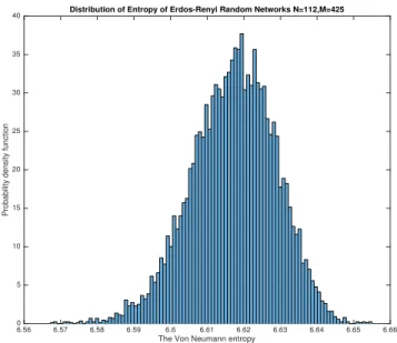
As we have previously stated, a random graph model defines a distribu-tion over graphs on a certain space of graphs. Specifically, the Erd˝os-Rényi random graph model defines a uniform distribution over graphs withN ver-tices andM edges. This distribution over graphs induces a distribution over the Von Neumann entropy of graphs, and we can run numerical simulations for a large number of times to obtain an empirical distribution over Von Neumann entropy of graphs to approximate the theoretical distribution over the Von Neumann entropy of Erd˝os-Rényi random graphs of same sizes. For this numerical simulation, we generate T = 10000 samples of Erd˝os-Rényi random networks and plot the estimated probability density function of the Von Neumann entropy of Erd˝os-Rényi random network samples.

6.56 6.57 6.58 6.59 6.6 6.61 6.62 6.63 6.64 6.65 6.66 The Von Neumann entropy

0 5 10 15 20 25 30 35 40

Probability density function

Distribution of Entropy of Erdos-Renyi Random Networks N=112,M=425

(10)

As we can see, in Figure 1, the Von Neumann entropy of Erd˝os-Rényi random networks with N = 112 vertices and M = 425 edges are mostly in the range of [6.57,6.66]. However, as we will see in the next numerical simulation, the Von Neumann entropy of an empirical network is usually smaller than almost all the Von Neumann entropy of networks generated by the Erd˝os-Rényi random graph model. In other words, the Von Neumann entropy of an empirical network typically has a small probability to be drawn from the distribution over Von Neumann entropy of Erd˝os-Rényi random graphs with the same number of vertices and edges. This indicates that the structure of an empirical network is typically different from the structure of networks generated by the Erd˝os-Rényi random graph model. To quantify this difference, we consider the expected hitting time of the Markov chain defined by the non-degree-preserving rewiring process. More specifically, for a given network, we are interested in the expected number of rewiring times needed until the Von Neumann entropy of the network undergoing non-degree-preserving rewiring falls within some range of the distribution over Von Neumann entropy of Erd˝os-Rényi random graphs of same sizes.

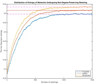
Now we present some numerical simulation results to visualize this pro-cess. The graph we use is the adjacency network of common adjectives and nouns in the novel David Copperfield by Charles Dickens [17]. Vertices rep-resent the most commonly occurring adjectives and nouns in the book, and edges represent any pair of words that occur in adjacent to one another in the book. The network hasN = 112 vertices andM = 425 edges. For each sim-ulation, we perform non-degree-preserving random rewiring for K = 1500 time steps, and we runT = 100 independent simulations. The blue, red and yellow curves represent the 5% quantile, median and 95% quantile of the empirical distribution over the Von Neumann entropy of rewired networks, respectively. The red and pink horizontal lines represent the median and 5% quantile, 95% quantile of the empirical distribution over the Von Neumann entropy of Erd˝os-R´enyi random networks of same size and density.

(11)

0 500 1000 1500 Number of rewirings

6.25 6.3 6.35 6.4 6.45 6.5 6.55 6.6 6.65

The Von Neumann entropy

Distribution of Entropy of Networks Undergoing Non-Degree-Preserving Rewiring

5-quantile median 95-quantile

Figure 2: The Von Neumann entropy of networks undergoing random rewiring

Neumann entropy of networks, we numerically observe that the distribution of rewired networks converges to the Erd˝os-R´enyi random graph ensemble. We note that such convergence would be otherwise difficult to observe.

4 A Matrix Perturbation Method to Estimate the

Expected Hitting Time

In the previous section, we performed numerical experiments to study the hitting time of non-degree-preserving rewiring process. However, this ap-proach is generally not computationally efficient, especially when the graph is large. Therefore, for the remainder of this research we will seek a way to estimate the expected hitting time given a graphGwithout performing ac-tual numerical simulations. In other words, we would like to find a function f(G) of a graph that approximates the empirical expected hitting time of the graphG.

(12)

rewired. To do so, we first develop perturbation analyses for the Laplacian matrix (Sec. 4.1) and its eigenvalues (Sec. 4.2) and eigenvectors (Sec. 4.3). We present a perturbation analysis of the Von Neumann entropy in Sec. 4.4, and introduce a functionf(G) to approximate the expected hitting time in Sec. 4.5.

Before continuing, we define some notations and constraints for our per-turbation analysis. Given an undirected, unweighted graph G withN ver-tices and M edges, let A denote the adjacency matrix of G, and Ddenote the degree matrix ofG. The Laplacian matrixL of the graph G is defined asL=D−A. Let L denote the Laplacian matrix before rewiring an edge (p, q) to (r, s), and L0 denote the Laplacian matrix after rewiring an edge (p, q) to (r, s). Then L0 =L+ ∆L. We assume the edges are not identical before and after one rewiring, namelyp6=q 6=r 6=s.

4.1 The Expected Value of the Difference Between Laplacian Matrices

The process of randomly rewiring an edge (p, q) to (r, s) can be decomposed into two steps. The first step is removing an edge (p, q) from the original graph G(0), resulting in an intermediate graph G(1). The second step is adding an edge (r, s) to the graphG(1), resulting in the rewired graphG(2). LetL(0)denote the Laplacian matrix of the original graphG(0),L(1)denote the Laplacian matrix of the intermediate graph G(1), and L(2) denote the Laplacian matrix of the rewired graphG(2), then we haveL(1)=L(0)+∆L(0), L(2)=L(1)+ ∆L(1). In terms of our previous notations, we have

L=L(0) ,L0=L(2) , ∆L= ∆L(0)+ ∆L(1)

4.1.1 Removing an edge

In this section we study how the Laplacian matrix changes due to the removal of an edge (p, q).

As we have stated previously, the elements of the Laplacian matrix L are given by

Lij =

  

 

Dii ifi=j

−1 ifi6=j and Aij =Aji= 1

0 otherwise

(13)

elements of ∆L(0)_ij are given by

∆L(0)_ij =

  

 

−1 ifi=j∈ {p, q}

1 ifi∈ {p, q}and j∈ {p, q} \i 0 otherwise

Hence the expected value of ∆L(0)_ij is given by

E[∆L(0)_ij ] =

(

P(p=iorq =i)×(−1) ifi=j P((p=iandq =j) or (p=j and q=i))×1 ifi6=j Since there are M edges in total, and we can only remove an edge when Aij =Aji= 1, we can write down the probabilities as

P(p=iorq =i) = di M and

P((p=iand q =j) or (p=j and q=i)) = Aij M

After substituting these probabilities into the previous equation, we have

E[∆L(0)_ij ] =

( −di

M ifi=j Aij

M ifi6=j

(1)

4.1.2 Adding an edge

In this section we study how the Laplacian matrix changes due to the addi-tion of an edge (r, s).

Since adding an edge (r, s) means Ars =Asr changes from 0 to 1, the

elements of ∆L(1)_ij are given by

∆L(1)_ij =

  

 

1 ifi=j ∈ {r, s}

−1 ifi∈ {r, s}and j∈ {r, s} \i 0 otherwise

Hence the expected value of ∆L(1)_ij is given by

E[∆L(1)_ij ] =

(

(14)

Since there are N(N₂−1) possible edges in total for a graph with N vertices, and we can only add an edge when Aij = Aji = 0, and {i, j} 6= {p, q}.

Therefore, there are N(N₂−1)−Mpossible edges to add. LetR = N(N₂−1)−M, then we can write down the probabilities as

P(r=iors=i) = N −1−di R and

P((r=iands=j) or (r=j ands=i)) = 1−Aij R

After substituting these probabilities into the previous equation, we have

E[∆L(1)_ij ] =

(_N₋₁₋_d

i

R ifi=j

−1−Aij

R ifi6=j

(2)

4.1.3 Rewiring an edge

In this section we study how the Laplacian matrix changes due to the rewiring of an edge (p, q) to (r, s). Since rewiring an edge can be decom-posed into removing an edge and adding an edge, we can simply combine the results in previous sections and write down a formula forE[∆Lij].

By the linearity of expectation, we have

E[∆L] =E[∆L(0)] +E[∆L(1)] (3)

We substitute Eqs. 1 and 2 into 3 to obtain

E[∆Lij] =

 



N−1−di N(N−1)

2 −M

− di

M ifi=j Aij

M −

1−Aij N(N−1)

2 −M

ifi6=j (4)

4.1.4 Linear approximation of rewiring multiple times

In previous sections we derived the formula to compute the expected value of the difference between Laplacian matrices before and after rewiring one time. We can use linear approximation to approximate the expected value of the difference between Laplacian matrices before and after rewiring multiple times. LetL0 denote the original Laplacian matrix before any rewiring, and

Ln denote the Laplacian matrix after rewiringntimes, then

E[(Ln−L0)ij]≈E[n∆Lij] =

 



n( N−1−di N(N−1)

2 −M

− di

M) ifi=j

n(Aij

M −

1−Aij N(N−1)

2 −M

(15)

Now we present some numerical simulation results to support our theo-retical results. The graph we use is the same as the graph used in previous numerical simulations. It hasN = 112 vertices andM = 425 edges.

First, we ran numerical simulations to compute E[∆Lij] by choosing

three specific entries (i, j). The first entry (51,51) is on the diagonal, the second entry (22,19) is not on the diagonal and corresponds to an edge, and the third entry (88,59) is not on the diagonal and does not correspond to an edge. For each choice for the number of rewires,n, we computed the mean across T = 10000 simulations. We plot the results for this experiment in Figure 3 and Figure 4. The straight lines represent the theoretical prediction according to Eq. (5), and the symbols and error bars represent the mean values and standard errors that we observe, respectively.

Next we ran numerical simulations to compute||E[∆L]||F, where|| · ||F

is the matrix Frobenius norm. For each choice of the number of rewires, n, we computed the mean across T = 10000 simulations, and we plot the results in Figure 5. The straight line represents the theoretical prediction according to Eq. (5), and the X symbols represent the observed values.

4.2 The Expected Value of the Difference Between Eigenval-ues of Laplacian Matrices

In this section we will use matrix perturbation theory to derive a relationship between E[∆L], the expected difference between Laplacian matrices, and

E[∆λi], the expected difference between eigenvalues of Laplacian matrices.

The central idea is to use a small perturbation to the adjacency matrix of the graph to approximate the process of randomly rewiring an edge of a graph. However, whether such approximation will be sufficiently accurate or not depends on the size and density of the graph, and intuitively we would expect that the approximation will be more accurate for large dense graphs. Throughout this section we will use ∆L, ∆λi, and ∆vi to denote the

ac-tual difference between the Laplacian matrices, eigenvalues of the Laplacian matrices, and eigenvectors of the Laplacian matrices before and after one rewiring, and we will useδL, δλi, andδvi to denote the difference between

the Laplacian matrices, eigenvalues of the Laplacian matrices, and eigenvec-tors of the Laplacian matrices before and after one small perturbation.

Let λi and vi denote the i-th eigenvalue and the associated unit

eigen-vector of a Laplacian matrixL, then we have Lvi =λivi

(16)

0 5 10 15 20 25 30 35 Number of rewirings

-0.6 -0.5 -0.4 -0.3 -0.2 -0.1 0

E

[

∆

Lij

]

Difference of Specfic Entries of Laplacian Matrices Undergoing Rewiring

Figure 3: E[∆Lij] for (i, j) = (51,51)

0 5 10 15 20 25 30 35

Number of rewirings -0.01

0 0.01 0.02 0.03 0.04 0.05 0.06 0.07 0.08

E

[

∆

Lij

]

Difference of Specfic Entries of Laplacian Matrices Undergoing Rewiring

Figure 4: E[∆Lij] for (i, j) = (22,19) and

(88,59)

(17)

0 5 10 15 20 25 30 Number of rewirings

0 1 2 3 4 5 6

||

E

[

∆

L

]

||F

Norm of Difference of Laplacian Matrices Undergoing Rewiring

Figure 5: ||E[∆L]||_F for different number of rewirings

LetδL=L0−L,δλi =λ0i−λi, andδvi=v0i−vi, then the previous equation

is equivalent to

(L+δL)(vi+δvi) = (λi+δλi)(vi+δvi)

After expanding both sides of the equation, we have

Lvi+Lδvi+δLvi+δLδvi=λivi+λiδvi+δλivi+δλiδvi

Since Lvi = λivi, and we can discard higher order delta terms δLδvi and

δλiδvi. the previous equation reduces to

Lδvi+δLvi =λiδvi+δλivi

MultiplyingvT_i on both sides, we have

v_iT(Lδvi+δLvi) =viT(λiδvi+δλivi) (6)

Since L is symmetric, we have vT_i L= (Lvi)T = (λivi)T =vTi λi. Hence

(18)

Sincevi is a unit vector, we have

v_iT(λiδvi+δλivi) =λvTi δvi+δλiviTvi =λiviTδvi+δλi (8)

Plugging equations 7 and 8 into equation 6, we have

δλi=vTi δLvi

Since ∆λi≈δλi, ∆L≈δL, we have

∆λi≈vTi ∆Lvi

E[∆λi]≈E[vTi ∆Lvi] =viTE[∆L]vi

Now we present some numerical simulation results. The graph we use is the same as the graph used in previous simulations, and it is a relatively small graph with N = 112 vertices andM = 425 edges. As we have stated before, small perturbation to the adjacency matrix is only an approximation of the process of randomly rewiring an edge of a graph, and there are mainly two ways to account for this fact and test if our estimation becomes more and more accurate as the process of randomly rewiring an edge becomes more and more “close” to a small perturbation. The first way is to run simulations on graphs of different sizes, and ideally we would like to see our estimation becomes more and more accurate as the size and density of the graph becomes larger and larger. However, this method requires computing the eigenvalues of large matrices, which is time-consuming if we want to run simulations for a large number of times. The second way is to introduce a constant to control the magnitude of the perturbation, and it is the way we will use. Specifically, given the original adjacency matrix A(0), first we randomly rewire an edge and obtain a new adjacency matrix A(1). Then we manually shrink ∆A=A(1)−A(0) by a factor ofby setting A(2) = A(0)+(A(1)−A(0)). We consider A(2) as the resulting adjacency matrix after a small perturbation is applied to A(0), and by linearity of expectation we can write down the expected value of the difference between Laplacian matrices as

E[L(2)−L(0)] =E[L(1)−L(0)] =

 



( N−1−di N(N−1)

2 −M

− di

M) ifi=j

(Aij

M −

1−Aij N(N−1)

2 −M

(19)

If we let = 1, then the result is the same as randomly rewiring an edge. However, we can also let <1, such as = 0.1, and we would expect our estimation to become more accurate, because a smaller means a smaller perturbation.

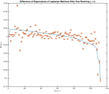
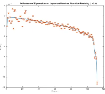
In our numerical simulations, we try three different values of , namely = 1, = 0.1 and = 0.01, and we compare the results to see if our estimation becomes more accurate as decreases from = 1 to = 0.01. For each simulation, we compute ∆λi for every entry i, and we run the

simulation for T = 10000 times. The blue line represents the theoretical values E[∆λi], and the symbols and error bars represent the mean values

and standard errors of the simulation results.

0 20 40 60 80 100 120

Entryi

-0.12 -0.1 -0.08 -0.06 -0.04 -0.02 0 0.02 0.04 0.06 0.08

E

[

∆

λi

]

Difference of Eigenvalues of Laplacian Matrices After One Rewiring (ǫ=1)

Figure 6: E[∆λi] for all entryiwhen = 1

As we can see, in Figure 6, when = 1, our estimation of E[∆λi] based

(20)

0 20 40 60 80 100 120

Entryi

-12 -10 -8 -6 -4 -2 0 2 4

E

[

∆

λi

]

×10-3 Difference of Eigenvalues of Laplacian Matrices After One Rewiring (ǫ=0.1)

Figure 7: E[∆λi] for all entry iwhen = 0.1

0 20 40 60 80 100 120

Entryi

-12 -10 -8 -6 -4 -2 0 2 4

E

[

∆

λi

]

×10-4 Difference of Eigenvalues of Laplacian Matrices After One Rewiring (ǫ=0.01)

(21)

4.3 The Expected Value of the Difference Between Eigen-vectors of Laplacian Matrices

In this section we will continue using matrix perturbation theory to derive a relationship between ∆L, the expected value of the difference between Lapla-cian matrices, ∆λi, the expected value of the difference between eigenvalues

of Laplacian matrices, and ∆vi the expected value of the difference between

eigenvectors of Laplacian matrices.

Using the notations defined in the previous section, we have

Lδvi+δLvi =λiδvi+δλivi

Hence

(L−λiI)δvi= (δλiI−δL)vi (9)

Now we consider the singular matrix L−λiI. Let Λ = diag(λ1,· · · , λn)

and V = [v1· · ·vn] where each vi is a column unit eigenvector, then by the

spectral theorem, since Lis symmetric, we can decompose L as

L=VΛVT =

n

X

j=1

λjvjvjT

SinceVTV =V VT =I, we have

L−λiI =V(Λ−λiI)VT =

X

j6=i

(λj−λi)vjvTj

Define pseudoinverse of the matrixL−λiI as

(L−λiI)+=

X

j6=i

1 (λj−λi)

vjvjT

Then after left multiplying equation 9 by (L−λiI)+, we have

δvi = (L−λiI)+(δλiI−δL)vi

Since ∆vi ≈δvi, ∆λi ≈δλi, ∆L≈δL, we have

∆vi≈(L−λiI)+(∆λiI−∆L)vi

E[∆vi] = (L−λiI)+E[∆λiI−∆L]vi

=X

j6=i

1 (λj −λi)

vjvjT(E[∆λi]I−E[∆L])vi

=X

j6=i

v_jTE[∆L]vi

(λi−λj)

vj

(22)

Although this result is not used in deriving E[∆h], we note that it can be useful for deriving equations for other measurements of a graph.

4.4 The Expected Value of the Difference Between Von Neu-mann Entropies

In this section we will use the results in previous sections to drive a rela-tionship between ∆h, the difference between the Von Neumann entropy of the graphs, and ∆λi, the difference between eigenvalues of Laplacian

matri-ces. Note that in previous sections when we derive the formula for the Von Neumann entropyh of a graph Gas

h=−

N

X

i=1

λilog2(λi)

theλi are the eigenvalues of the rescaled Laplacian matrix ₂_M1 L. If we use

the notations defined in previous matrix perturbation sections, we would have

h=−

N

X

i=1

λi

2M log2( λi

2M) whereλi are the eigenvalues of the Laplacian matrixL.

Let h and h0 denote the Von Neumann entropy of a graph before and after one small perturbation, and using the notations defined in the previous sections, we have

h=−

N

X

i=1

λi

2M log2( λi

2M) and

h0=−

N

X

i=1

λi

2M + δλi 2M log₂ λi

2M + δλi

2M

Using first order Taylor series approximation, we have

λi

2M + δλi 2M log₂ λi

2M + δλi

2M

≈ λi

2M log2( λi

2M)+ δλi

2M

log₂( λi 2M) +

1 ln(2)

Sinceδh=h0−h, we have

δh≈ −

N X i=1 δλi 2M

log₂( λi 2M) +

1 ln(2)

(23)

Since ∆λ≈δλ,δh≈∆h, we have

∆h≈ −

N

X

i=1

∆λi

2M

log₂( λi 2M) +

1 ln(2)

E[∆h]≈ −

N

X

i=1

E[∆λi]

2M

log₂( λi 2M) +

1 ln(2)

(11)

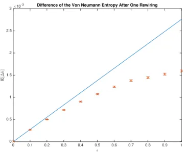
Now we present some numerical simulation results. The graph we use is the same as the graph used in previous simulations, and it has N = 112 vertices andM = 425 edges. Similar to what we did in previous numerical simulations, we use a constant to control the perturbation magnitude, and we try different values of to see if our estimations become more and more accurate as decreases. For each value of , we run the simulation forT = 10000 times. The blue line represents the theoretical values E[∆h], and the red symbols and error bars represent the mean values and standard errors of the simulation results.

0 0.1 0.2 0.3 0.4 0.5 0.6 0.7 0.8 0.9 1

ǫ 0

0.5 1 1.5 2 2.5 3

E

[

∆

h

]

×10-3 _{Difference of the Von Neumann Entropy After One Rewiring}

Figure 9: E[∆h] for different values of

(24)

is not very accurate. One possible reason is that the size of the graph is not large enough, and therefore randomly rewiring an edge of the graph cannot be accurately modeled as a “small perturbation”. However, when gradually decreases, our estimation becomes more and more accurate, and this result confirms our expectation that the smaller the perturbation, the more accurate our estimation ofE[∆h] becomes.

4.5 Estimation of the Expected Hitting Time

In this section we use the results from previous sections to estimate the expected hitting time. For a given graph withN vertices and M edges, let h denote its Von Neumann entropy, and let h(.05) denote the 5% quantile of the empirical distribution over Von Neumann entropy of Erd˝os-R´enyi random graphs with N vertices and M edges. We are interested in the expected number of non-degree preserving rewiring times needed until the Von Neumann entropy of the rewired graph is no less than h(.05), and one natural estimation would be

f(G) = h

(.05)₋_h

E[∆h]

The intuition is that the Von Neumann entropy of a graph is expected to increase by E[∆h] after one random rewiring, and if the Von Neumann entropy of a graph is constantly increasing at this rate, then the number of non-degree preserving rewiring times needed until the Von Neumann entropy of the rewired graph is no less thanh(.05)is simply the difference between the target Von Neumann entropy and the initial Von Neumann entropy divided by the increasing rate.

However, we would expect that our estimation of the expected hitting time would be smaller than the actual value obtained from numerical simu-lation, because as we can see from Figure 2, the increasing rate of the Von Neumann entropy E[∆h] of the network undergoing rewiring is decreasing as the number of rewiring times increases.

(25)

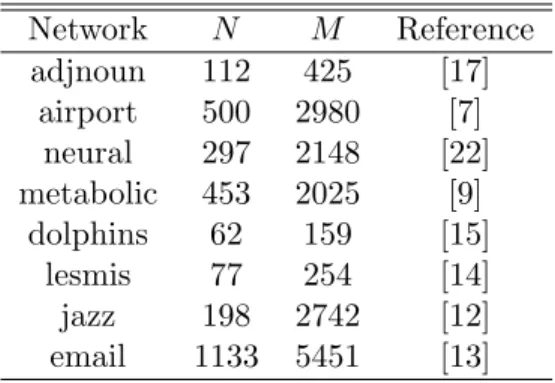
Network N M Reference

adjnoun 112 425 [17]

airport 500 2980 [7]

neural 297 2148 [22]

metabolic 453 2025 [9]

dolphins 62 159 [15]

lesmis 77 254 [14]

jazz 198 2742 [12]

email 1133 5451 [13]

Table 1: Basic summary statistics for the networks that we use for this numerical simulation. The number of vertices is denoted by N, and the number of edges is denoted byM.

rewired, because computing the Von Neumann entropy of a graph requires computing all the eigenvalues of a graph, and the runtime of performing this operation for millions of times is too large. Instead, we compute the Von Neumann entropy of the rewiring graph for every 10dN/100)erewirings. This trick greatly reduces the runtime of the numerical simulation, because the number of times of computing all the eigenvalues of a graph is reduced by a factor of 10dN/100)e. Although it also increases the variance of the sample mean estimator, the standard error of the sample mean divided by sample mean is no larger than 0.05, which indicates that the sample mean should be close enough to the true expected hitting time.

(26)

0 200 400 600 800 1000 1200 1400 1600 1800 2000 Estimation

-2000 0 2000 4000 6000 8000 10000 12000 14000

Simulation

Hitting Time: Simulation vs. Estimation

adjnoun airport neural metabolic dolphins lesmis jazz email

Figure 10: Comparison of the sample mean of actual hitting times and our estimation h_E(.05)_[∆_h−_]h for networks of different sizes

5 Conclusion

In this paper, we used the concept of the Von Neumann entropy of a graph to define a hitting time for non-degree-preserving random rewiring process, which is the number of rewiring times needed until the Von Neumann en-tropy for the rewired graph is larger than 5% quantile of the distribution over the Von Neumann entropy of Erd˝os-R´enyi random networks. Since the purpose of defining the hitting time is to quantify the difference between a given network and networks generated by the Erd˝os-R´enyi random graph model with the same number of vertices and edges, we do not really need to find an approximation of the actual value of the expected hitting time. Instead, we only need to give an estimation that is positively correlated with the expected hitting time, and we used

f(G) = h

(.05)₋_h

E[∆h]

(27)

ran-dom rewiring as given by Eq. (11). The intuition behind our estimation f(G) is a simple linear approximation, and we expect that a more accurate estimation can be derived by using more complicated models such as an exponential model to model the trajectories of the Von Neumann entropy of networks undergoing rewiring. Experimental results show that our esti-mation is highly correlated with the sample mean of the actual hitting time obtained from numerical simulation, and the advantage of using our estima-tion is that it can be computed directly without performing a large number of simulations and taking the sample mean of the actual hitting times.

The central part of the estimation isE[∆h], which is obtained by using a small perturbation to the adjacency matrix of the graph to approximate one random rewiring of a graph, and then applying matrix perturbation techniques to derive equations for E[∆L], E[∆λi], and E[∆h]. However,

(28)

Bibliography

[1] Réka Albert and Albert-László Barabási. Statistical mechanics of com-plex networks. Reviews of Modern Physics, 74(1):47, 2002.

[2] Albert-László Barabási and Réka Albert. Emergence of scaling in ran-dom networks. Science, 286(5439):509–512, 1999.

[3] András Békéssy, P Bekessy, and János Komlós. Asymptotic enumera-tion of regular matrices. Stud. Sci. Math. Hungar, 7:343–353, 1972.

[4] B´ela Bollob´as. Modern Graph Theory, volume 184. Springer Science & Business Media, 2013.

[5] Samuel L Braunstein, Sibasish Ghosh, and Simone Severini. The lapla-cian of a graph as a density matrix: a basic combinatorial approach to separability of mixed states. Annals of Combinatorics, 10(3):291–317, 2006.

[6] Fan RK Chung. Spectral Graph Theory, volume 92. American Mathe-matical Soc., 1997.

[7] Vittoria Colizza, Romualdo Pastor-Satorras, and Alessandro Vespig-nani. Reaction–diffusion processes and metapopulation models in het-erogeneous networks. Nature Physics, 3(4):276–282, 2007.

[8] Manlio De Domenico, Vincenzo Nicosia, Alexandre Arenas, and Vito Latora. Structural reducibility of multilayer networks. Nature

Commu-nications, 6, 2015.

[9] Jordi Duch and Alex Arenas. Community detection in complex net-works using extremal optimization. Physical Review E, 72(2):027104, 2005.

[10] Paul Erd6s and A R´enyi. On the evolution of random graphs. Publ.

Math. Inst. Hungar. Acad. Sci, 5:17–61, 1960.

[11] Miroslav Fiedler. Laplacian of graphs and algebraic connectivity.

Ba-nach Center Publications, 25(1):57–70, 1989.

[12] Pablo M Gleiser and Leon Danon. Community structure in jazz.

(29)

[13] Roger Guimera, Leon Danon, Albert Diaz-Guilera, Francesc Giralt, and Alex Arenas. Self-similar community structure in a network of human interactions. Physical Review E, 68(6):065103, 2003.

[14] Donald Ervin Knuth, Donald Ervin Knuth, and Donald Ervin Knuth.

The Stanford GraphBase: A Platform for Combinatorial Computing,

volume 37. Addison-Wesley Reading, 1993.

[15] David Lusseau, Karsten Schneider, Oliver J Boisseau, Patti Haase, Elis-abeth Slooten, and Steve M Dawson. The bottlenose dolphin commu-nity of doubtful sound features a large proportion of long-lasting asso-ciations. Behavioral Ecology and Sociobiology, 54(4):396–405, 2003.

[16] Stephen B Maurer. Matrix generalizations of some theorems on trees, cycles and cocycles in graphs. SIAM Journal on Applied Mathematics, 30(1):143–148, 1976.

[17] Mark EJ Newman. Finding community structure in networks using the eigenvectors of matrices. Physical Review E, 74(3):036104, 2006.

[18] Filippo Passerini and Simone Severini. The von neumann entropy of networks. Available at SSRN 1382662, 2008.

[19] Louis M Pecora and Thomas L Carroll. Master stability functions for synchronized coupled systems. Physical Review Letters, 80(10):2109, 1998.

[20] Per Sebastian Skardal, Dane Taylor, and Jie Sun. Optimal synchro-nization of complex networks. Physical Review Letters, 113(14):144101, 2014.

[21] Gilbert W. Stewart and Ji guang Sun. Matrix Perturbation Theory. Academic Press, 1990.