Abstract
The goal of Honors project was to modify an in situ Nitrate/Nitrite autoanalyzer to enable in situ measurements of Soluble Reactive Phosphates (SRP). The purpose for this project was to create instrumentation able to determine concentrations of SRP, a crucial nutrient element for both freshwater and marine environments. The Redfield atomic ratio of plankton averages approximately 106 C: 16 N: 1 P and has often been used to determine whether the limiting element needed for primary production is N or P. Improved technologies for rapid, in situ determination of SRP concentrations are needed. One of two Nitrate/Nitrite analyzers in our laboratory was redesigned to accurately measure the SRP at nanomolar concentrations. The analyzer, a Mini Spectrophotometric Elemental Analysis System (M-SEAS), utilized a molybdate-based color reagent to react with SRP in water samples followed by absorbance at 680, 700, and 720 nm wavelengths. Using a system of peristaltic pumps, the M-SEAS, was able to reproducibly measure SRP concentrations down to 80 ± 9.6 nM PO43-. As a result of the experiment additional nutrient analysis of marine samples can be conducted to better understand biological and geochemical cycling in the environment.
Introduction
Nitrogen andPhosphorus are essential nutrient elements in all aquatic ecosystems, needed
for growth and cell maintenance by all phytoplankton and all other photosynthesizing organisms.
Accurate analysis of Dissolved Inorganic Nitrogen (DIN) and Soluble Reactive Phosphates (SRP)
generally present at low concentrations in natural waters allows researchers to monitor chemical
conditions that control the growth of these microorganisms, providing information which can be
used in predictive models supported by larger scale data sets. In natural waters, the microbial
growth is limited by either nitrogen or phosphorus.5 The identity of the primary growth limiting nutrient can be generally predicted by DIN:SRP ratios in the water column.3 A combination of DIN and SRP measurements compared to the Redfield ratio of 106:16:1, the average
stoichiometric atomic ratio of carbon, nitrogen, and phosphorus respectively found for living
phytoplankton cells, is generally used to determine whether N or P is limiting.5 A deviation in DIN/SRP ratio from the Redfield ratio leads to a prediction for which is the limiting nutrient.
Hoyer et al. (2002) describe the significant correlation between chlorophyll-a concentrations and Total Nitrogen (TN) and Total Phosphorus (TP) in Florida coastal waters. Although, TP accounts
for all the P in the environment, the components of dissolved or particulate P compounds which
which only accounts for approximately 8% of TP.7 Measuring the ratio of the nutrients not only helps to understand eutrophication but how nutrient loading and cycling occurs in the environment.
Researchers have sought instrumentation that can be utilized to measure the concentrations of N
and P in situ because of difficulties and measurement inaccuracies encountered with stored
samples. Recent instrumentation development in the Robert Byrne laboratory at the University of
South Florida, conducted in collaboration with the Martens laboratory in the Department of Marine
Sciences at UNC-Chapel Hill, has provided several new varieties of prototype in situ nutrient
element analyzers. The Spectrophotometric Elemental Analysis System (SEAS) prototypes are the
first set of available instruments designed for in situ underwater nutrient analyses but are still in
beta-phase testing.
The SEAS instrumentation utilizes Beer’s Law in order to calculate the absorption of SRP.
The SRP in a sample reacts with a molybdenum blue color reagent which can then be measured
through absorption of light. The fundamentals of Beer’s Law consider the quantitative measure of
radiative energy when striking the detector over time, P. If the radiative power is described as a
beam of light then the number of absorbing units, N, can describe the relative concentration of
absorbing units in the solution. As the number of absorbing units changes the power striking the
detector also changes, ΔP = −k ∗ P ∗ ΔN, where k is the proportionality constant of absorbance.
Integrating the equation to solve for total absorbance in terms of the number of absorbing units
leaves the equation ln (𝑃𝑃
0) = −𝑘 ∗ 𝑁 where P0 is the radiative power measured by the detector when no absorbing units are present. To determine the concentration of absorbing units, we must
consider the path in which the sample is passed when the incident light strikes the sample as well
as a factor of Avogadro’s Number,N = c ∗ (6.02 ∗ 1023) ∗ b ∗1000s , where c is the molar
equation into the previous equation and converting the power ratio into Briggsian logarithms gives
returns 𝑙𝑜𝑔𝑃𝑃0= 𝜀𝑏𝑐 = A, where ε is the molar absorptivity of the absorbing molecule and A is the
absorbance. Using these equations the concentration of phosphates can be determined by the SEAS
instrument.10
Dissolved nitrate plus nitrite (NOx-), ammonium (NH4+), and SRP are the three main compounds of these two elements which can be directly utilized by phytoplankton. The most
current SEAS instrumentation, the mini-SEAS (M-SEAS), has been utilized at UNC during the
past year for NOx- analysis. However, the Martens lab has lacked access SRP analysis using in situ SEAS technology. The project described in this report sought to develop an underwater, in
situ SRP analyzer using similar technology. The M-SEAS instrumentation currently used for NOx -measurements was altered in order to measure SRP in situ based upon methodology previously
proposed by Lori Adornato at the University of South Florida.1 In order to complete this project, the M-SEAS SRP analyzer was set up to use the same electronic configuration currently in the
nitrate analyzer, however, the flow structure and chemical methodology had to be altered.
Improving analytical precision and lowering the limit of detection to environmental concentrations
became important objectives for this project.
The primary goal of the project was to develop an instrument that could be used in
conjunction with the existing NOx- analyzer in order to be able to obtain simultaneous concentration and water column depth profiles for both nutrients. The Martens lab has previously
utilized the NOx-analyzer to measure how sponges with high microbial abundance (HMA) in their tissues have impacted nitrogen cycling in Florida Bay water, specifically with conversion of
both processes. After collecting and analyzing this data, it was determined that the next step would
be to understand the role of sponges in P cycling in the system, specifically conversion of organic
P compounds to SRP. In addition to allowing pursuit of this question, the creation of an SRP
analyzer will allow for a larger understanding of how inorganic P absorption and desorption might
impact both recycling and availability in dissolved form. Benitez-Nelson (2000), suggests the long
turnover rate of P might be due to the lack of bioavailability or that the nutrient is needed at a
constant rate.
Procedure
In order to quantify the concentration of SRP using Beer’s Law, samples are mixed with a
color reagent and a spectrophotometer is used to detect the absorbance of light by the sample.
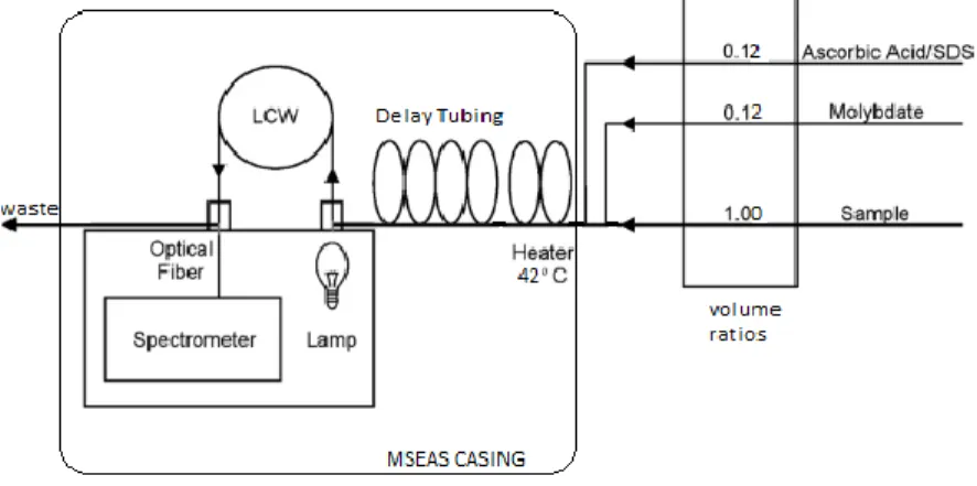
Figure 1 displays a schematic of the MSEAS instrumentation. The schematic shows the flow
diagram of the sample and volumetric ratios for proper analysis using this methodology. The mixed
reagents and solution is then heated by a heating coil so the mixed solution heats to 30° C for the
completion of the reaction. The sample then reacts in a delay tubing before detection by a
spectrophotometer at 680, 700, and 720 nm wavelengths. Finally, the mixed solution is pumped
out of the instrument and can be released in the water should the experiment be conducted in situ.
Reagent Preparation
The color reagent methodology is based upon work with liquid waveguides conducted by
Zhang and Chi (2002) at the University of Miami. In order to determine the concentration of PO4 3-in the sample, the reaction between the color reagent, ascorbic acid, and phosphate produces a dark
blue solution which absorbs in the visible range between 650 - 750 nm wavelengths.2 The determination of phosphate is based on the formation of a 12-molybdophosphoric acid from the
reaction between the phosphate and molybdate. This solution is then reduced by ascorbic acid in
a two electron step reduction to form a blue heteropoly phosphomolybdate complex.9 An ammonium molybdate solution ((NH4)6Mo7O24 · 4H2O) was used in order to provided dissociated molybdate anions, when reacted with an Antimony Potassium Tartrate solution, to react with the
sample phosphates. In acidic environments the Mo(IV) exists as a dimer, however upon mixing
aqueous solutions of phosphate, Mo(VI), and sulfuric acid the 12-molybdophosphoric acid rapidly
forms. The fundamental reaction conducted during the delay tubing follows the equation:
H3PO4 + 5 Mo(IV) ↔ (12-molybdophosphoric acid) + 7 H+
It was determined that the stoichiometric measurements of the amount of blue product formed
did not influence the acidity of the solution as long as the acidity is high enough to prevent the
direct reduction of Mo(VI).9 After the reduction by ascorbic acid, the blue complex is formed and the blue phosphomolybdate absorbance can be measured.
In order to prepare the solution needed for the measure of the concentration of phosphate,
the follow procedure was followed. All glassware used in the analysis is prepared by soaking a 2%
HCl acid bath for at least six hours, followed by rinsing in a combination of DI and 18.2Ω
rinsed three times with B-water before use. To prepare the color reagent stocks, 3.0 grams of
antimony potassium tartrate was dissolved in 1.0 L of B-water. Stock ammonium molybdate was
prepared by dissolving 2.3g ammonium molybdate in 192 mL of 5 N H2SO4. The 5 N H2SO4 was prepared by adding 26.88 mL of concentrated 36.0 N H2SO4 in 165.12 B-water. To complete the color reagent, 50 mL stock antimony potassium tartrate was added to 192 mL stock ammonium
molybdate then diluted to 1.0 L with B-water, for smaller sample counts the reagent was made in
smaller equimolar volumes. An ascorbic acid solution is used to acidify the sample and initiate the
reaction of the sample with the molybdate solution. The ascorbic acid solution is prepared by
dissolving 0.50 g of ascorbic acid with 7.0 g sodium dodecyl sulfate in 100 mL.
The stock potassium dihydrogen phosphate, used for a standard calibration, was prepared
by adding 0.1757 g of KH2PO4 (MW = 136.086 g
mol) in 1 Liter of B-water to create a 1290 µM
PO43- solution. This stock solution undergoes serial dilution in order to achieve the much lower concentrations generally found under oligotrophic conditions.2 However in order to calibrate the instrument for the purposes of the present project, higher concentrations will be used. The stock
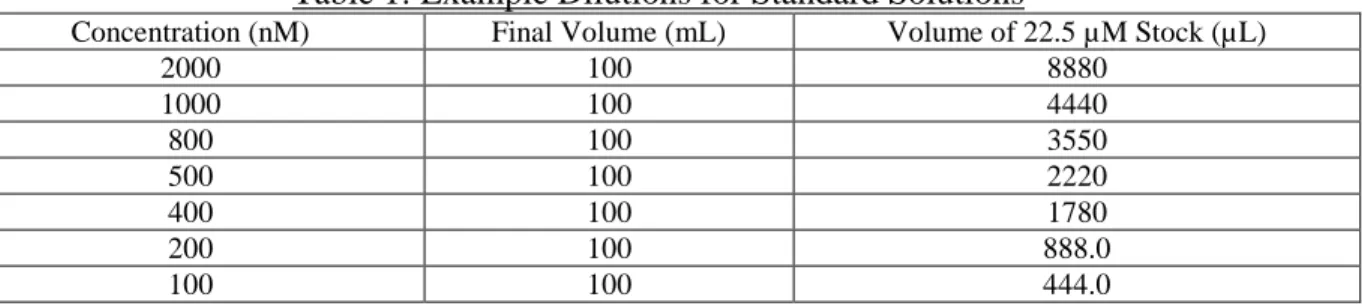
solution is diluted to 22.5 µM PO43- by adding 1750 µL and dilute to 100 mL. Examples of preliminary final dilutions used for calibration of the instrument are listed in Table 1.
Table 1: Example Dilutions for Standard Solutions
Concentration (nM) Final Volume (mL) Volume of 22.5 µM Stock (µL)
2000 100 8880
1000 100 4440
800 100 3550
500 100 2220
400 100 1780
200 100 888.0
Discussion
Standard Curve Analysis – October 22, 2015
For the initial tests of the M-SEAS SRP analyzer, the standards were added to BioPharm
BPT tubing at a rate of 3.03 mL/min and the color reagent and ascorbic acid were added at 0.38
mL/min each through peristaltic pumps. The 15 cm length of tubing which carries the sample
passes over a heating coil which was set to 30o C as recommended by Adornato (2007) to increase the rate of the reaction.1 The inner diameter of the tubing at the heating coil is 3mm. Sample Calculation 1 was used in order to quantify the length of tubing needed to allow completion of the
90 second reaction after heating.2 Using the result from Sample Calculation 1, 80.5 cm of BPT tubing was placed after the heating coil, but before the sample was passed through the Liquid
Wave Guide (LCW) detector with an initial length of 22 cm.
Sample Calculation 1
Flow Rate =1
4× 𝜋 × inner diameter of tubing × velocity of water
3.79mL
min = 0.25 × 𝜋 × 0.3 cm × 𝑙 90 sec
𝑙 = 80.43 cm
During the first run of a standard curve on the MSEAS instrument, a B-water reference
spectrum from 450 nm to 750 nm wavelength was taken after rinsing the instrument for 180
seconds. After the reference was established the standard curve was run on a operation loop which
included a 240 second rinse with the sample and the color reagent/acidic solution, followed by 40
iterations of data collection at three wavelengths (680, 700, 720 nm), and a 20 second pump
disabled pause in order to switch the sample. The data was collected by the mainframe computer
the absorbance values in an excel spreadsheet. This excel spreadsheet was run through a Matlab
script I generated specifically for the analysis of SRP in the current data collection scheme. The
Matlab script converted the absorbance values into concentrations based on calibration curves,
such as shown in Figure 2. These calculated concentrations were plotted against the theoretical
standard values, Figure 3, in order to observe accuracy and precision of the instrument. The data
was also analyzed through time within each sample, Figure 4, to perceive how the absorbance may
be affected through time in the instrument, with the intention of adjusting delay times and pump
speeds. The calibration curve was created under high concentrations in order to focus on the
completion of the reactions as a function of pump speed before the issue of sensitivity was
investigated. The standards for the October 22 run were incorrectly prepared due to a conversion
and dissociation calculation error which was not recognized until a following iteration of the data.
However, the collected data could be analyzed since the standards were still made in equivalent
ratios even though the concentrations, and thus absorbance, were much higher than would be
detected for 400, 800, 2000, and 4000 nM concentrations.
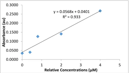
Figure 2: October 22 Calibration Curve. The data in this figure displays the calibration curve determined for the data collected on October 22, the absorbance values were collected at 700
y = 0.0568x + 0.0401 R² = 0.933
0.0000 0.0500 0.1000 0.1500 0.2000 0.2500 0.3000
0 1 2 3 4 5
A
b
sor
b
an
ce
(au
)
nm wavelength. The linear regression line was used as the calibration curve to find the concentration of the collected data points.
In addition to the miscalculation of the concentrations, the third point in the curve had an
absorbance much higher than expected. Ignoring this anomaly in the data the points in the
calibration curve is probably better represented by a quadratic curve than a linear fit. This result
suggests that the reaction is not be complete at the tube length used, heater temperature, or pump
speed or a combination of these factors. The calibration curve was used to determine SRP
concentration of the data, which is not the actual concentration due to the error but can be used as
an indicator of the accuracy and precision.
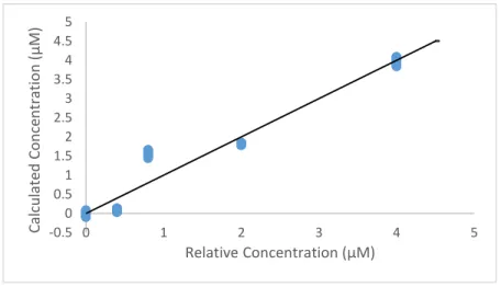
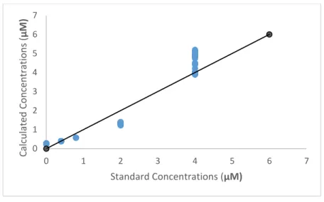
Figure 3: Accuracy and Precision analysis October 22. This graph displays the calculated ratio concentration against the ratio predicted standard concentration based on the calibration curve in Figure 2. The line represents the y=x line, the goal for the accuracy of the instrument.
The third set of collected data points are much higher than the y=x line (Figure 3), which
is expected due to the higher absorbance values. The second and fourth standard data points do not
reach the expected values due to an incomplete reaction. As a result of the data described in Figure
-0.5 0 0.5 1 1.5 2 2.5 3 3.5 4 4.5 5
0 1 2 3 4 5
Calcula
ted
Con
ce
n
tra
tio
n
(
µ
M)
2 and Figure 3, the length of tubing was extended by 20 cm to a total 100 cm between the heating
coil and the LCW. The temperature of the sample passing over the heating coil was analyzed.
Although the heating coil was set to 30 oC, the sample was not heated to this temperature in the short 15 cm contact. In order to have the sample heated to 30o C the heater needed to be set to 42o C.
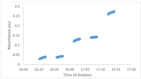
Figure 4: Absorbance as a Function of Time in the Standard Curve Calibration. The results show how the absorbance value changes for each set of standard iterations.
The data in Figure 4 illustrates that the absorbance within each standard increases
non-linearly over time within each sample, the concave down form of the lines indicates contamination
probably because the sample rinse was not completely through the LCW before data points were
collected for the next standard. Therefore, the delay time between the samples was increased from
240 to 420 seconds for future tests.
Standard Curve Analysis: November 3, 2015
Several calibration curves were obtained after the October 22 test using the adjusted
parameters and correct standard concentrations, all the standard analyses displayed an abnormal
0 0.05 0.1 0.15 0.2 0.25 0.3
16:04 16:19 16:33 16:48 17:02 17:16 17:31 17:45
Ab
so
rb
an
ce
(au
)
pattern in the blank (0 µM) standard. This pattern was not seen in the October 22data, however
the absorbance values were decreasing over time in the blank measurement, as shown by data in
Figure 5.
Figure 5: Absorbance vs Time – Blank Standard Analysis. The data in this figure displays the abnormal occurrence found repeatedly during data collection with correct standards and adjusted parameters.
The data presented in Figure 5 reveals the absorbance values continually decreased significantly through time during the data collection for the blank standard. Therefore, the average
blank absorbance value did not accurately reflect the true absorbance value. In order to improve
this aspect of the standard curve a second set of blank measurements was obtained. This alternate
blank measurement did not have the same decrease in absorbance in time, allowing for use in the
standard curve. The proposed reasoning for the occurrence found in Figure 5 is the ascorbic acid
solution has a soap-like texture and may not mix well initially with the sample. The mixing leaves
bubbles at junctions between the tubing of different sections in the MSEAS instrument. Such
0 0.0005 0.001 0.0015 0.002 0.0025 0.003 0.0035 0.004 0.0045
18:08:38 18:10:05 18:11:31 18:12:58 18:14:24 18:15:50
Ab
so
rb
an
ce
(au
)
bubbles upon entering the LCW would give false readings due to scattering. In order to avoid
bubbles at junctions, the tubing connectors were exchanged for larger flow connections.
Standard Curve Analysis: November 5, 2015
The data collected on November 5 included all parameter adjustments determined during
previous standard analyses. The standards were correctly prepared and data points were collected
for this run; however, the power supply tripped and only 5 data points were recorded for the 0.8
µM standard before the analysis was terminated. The standard calibration curve for the November
5 run is located in Figure 6.
Figure 6: Standard Calibration Curve – November 5.
Similar to the calibration curves in previous runs, such as shown by data in Figure 2, the
linear regression is not the best fit for data points. The non-linear curvature in the data indicate the
reaction was still not complete as the sample passed through the detector. In order to improve this
situation the pump speeds were adjusted to reduce the total flow rate of sample, color reagent, and
acid to 3.00 mL/min.
y = 0.225x - 0.0806 R² = 0.9438
-0.2000 0.0000 0.2000 0.4000 0.6000 0.8000 1.0000
0 1 2 3 4 5
A
b
sor
b
an
ce
(au
)
Figure 7: Calculated against Expected Concentrations – November 5.
Even though the linear regression of the standard curve was not the best quantitative
representation of the data, the concentrations for the absorbance were calculated based on the
Figure 6 calibration curve. Data seen in Figure 7 was utilized in order to analyze precision and
accuracy of the instrument with the line representing the ideal y=x line. From the data, the precision
of the lower standards was much higher than that of the higher concentrated standards, which could
occur because of the reaction not being completed fully or the linear regression being the wrong
fit for the data. Since the standard curve was a more important obstacle, this observation was
recorded for further analysis later once the standard curve was improved.
Reagent Analysis: November 9th, 2015
In order to save reagents and not create exorbitant waste, unused color reagent and ascorbic
acid solution were saved. Color reagent was stored in a 4o C refrigerator covered completely in tin foil to avoid light, while ascorbic acid was stored at room temperature because the solution
precipitates at temperatures lower than 17o C. After several standard curves were conducted with the same reagents that had aged, it was noted that the absorbance values were decreasing
0 1 2 3 4 5 6 7
0 1 2 3 4 5 6 7
C
alculat
ed
C
on
ce
n
trat
ion
s (
µM
)
significantly. If the absorbance values decrease too much, the slope of the linear regression reduces
making it harder to distinguish between minute concentrations. Therefore, on November 9, a
comparison between old and fresh color reagent and ascorbic acid was conducted by comparing
the standard curves of the data. The old reagent used was prepared two weeks prior to the analysis,
while the new reagent was prepared only hours before the analysis. Data presented in Figure 8
displays the results of the analysis. An analysis of the results shown in Figure 8, reveals that the
difference between using old reagent and new reagent was too great to ignore and so new was used
in further standard calibrations. Therefore, in order to reduce waste and have new reagents, only
100 mL of each reagent is prepared for each set of analyses. This 100 mL of reagent is sufficient
for up to 10 samples or standards.
Figure 8: Two Week Old and Fresh Reagents Comparison. This graph displays the standard curves between old and new reagents.
Standard Curve Analysis: November 20, 2015
The data collected on November 20 included all parameters adjusted from earlier tests of
the instrumentation including reagent age, pump speed, tubing length, and heating temperature.
y = 0.1822x - 0.0203 R² = 0.9798
y = 0.09x - 0.0116 R² = 0.9808
-0.0500 0.0000 0.0500 0.1000 0.1500 0.2000
0 0.5 1 1.5
A
b
sor
b
an
ce
(au
)
Standard Concentrations (µM)
New
The standard curve for this data is shown in Figure 9. During the experiment, the detection
reference was not an exact spectrum reference, because the blank exhibited a negative absorbance.
The reference could have been offset due to an air bubble trapped in one of the fittings.
Figure 9: Standard Curve – November 20.
An analysis of the data in the standard curve (Figure 9), reveals that the linearity of the
sample increased when the flow rate of the solution was reduced. However, the data still suggests
a slight quadratic behavior representative of insufficient completion of the reaction. Since the
sample is only heated momentarily on the heating coil and the rest of the tubing is located outside
the internal casing of the heating coil, the sample is subject to thermal cooling over the completion
of the reaction. In order to adjust for this cooling effect, the tubing was coiled inside the casing to
decrease the potential for heat loss through radiation from the heater. The linear regression of the
standard calibration curve was used to solve for the calculated concentrations of the data points
collected and Figure 10 displays the comparison with the standard concentrations.
y = 0.2424x - 0.0209 R² = 0.9798
-0.0500 0.0000 0.0500 0.1000 0.1500 0.2000 0.2500
0 0.5 1 1.5
A
b
sor
b
an
ce
(
µ
M
)
Figure 10: Calculated against standard concentrations- November 20. The dotted line represents the y=x line which represents the expected and ideal concentrations.
The results shown in Figure 10 display a comparison of calculated and expected
concentrations. Most of the standard exhibit strong accuracy, except for the 0.5 µM standard,
shown by the average point almost being equivalent to the dotted y=x line. The data points
revealed low precision which led to the data being insufficient for clear analysis. The imprecision
is greater at higher concentrations, especially at 1 µM, where the calculated concentrations range
from 0.78 to 1.69 µM. This imprecision allows for large variation in linear curve fits to the data.
In order to improve the precision the pathlength of the LCW has been extended to 42 cm, which
should help with the sensitivity of the instrument when lower concentrations are analyzed.
Standard Curve Analysis: December 1, 2015
A data set was obtained on December 1, which included all of the parameter adjustments
made thus far. While attempting to coil the 100 cm of reaction tubing in the instrument casing, the
fiber optic cable leading to the detector was damaged and had to be replaced with a cable which
0 0.2 0.4 0.6 0.8 1 1.2 1.4 1.6 1.8 2
0 0.2 0.4 0.6 0.8 1 1.2
Calcula
ted
Con
ce
n
tra
tio
n
s (
µ
M)
had a smaller circumference; therefore, the absorbance decreased and the integration time
increased from 1 ms, from other runs, to 37 ms. The standard calibration curve shown in Figure
11 was produced from this data set.
Figure 11: Standard Curve – December 1.
The standard curve of the data collected on December 1 is extremely linear with a R2 of 0.9979. This linear regression was used to produce calculated concentrations for the data in Figure
12.
Figure 12: Calculated against Standard Concentration – December 1. This graph displays the concentrations calculated from the linear regression and the absorbance values.
y = 0.1563x - 0.0123 R² = 0.9979
0.0000 0.0200 0.0400 0.0600 0.0800 0.1000 0.1200 0.1400 0.1600
0 0.5 1 1.5
A b sor b an ce (au )
Standard Concentrations (µM)
0 0.2 0.4 0.6 0.8 1 1.2 1.4
0 0.5 1 1.5
Calcula ted Con ce n tra tio n s ( µ M)
In the analysis of Figure 12, the precision of the data improved with all forty of the collected
points within a small range of a concentrations. The accuracy of the data is greatly improved yet
still drops off at higher concentrations, similar to the November 20 data. In order to improve the
accuracy of the data the pump speed will be further decreased in order to allow for maximal
completion of the reaction: the lower pump speed will be 1.89 mL/min. The reasoning behind the
decrease in pump speed, comes from Adornato and Kaltenbacher (2007) who used 473 seconds of
reaction time in comparison to the 90 seconds used by Zhang and Chi (2002), which will occur at
this lower pump speed.1,2
Figure 13: Absorbance against Time at 700 nm Wavelength.
The change in the absorbance for each standard in time is displayed in Figure 13. The
relatively linear fits represent good repetitions and consistent data. At this state, the instrument is
working well for standard concentrations between 100 nM – 1000 nM, however, the average
concentration of SRP in oligotrophic natural water is lower than these values. Therefore the
sensitivity of the instrument will need to be improved because the absorbance values between the
blank and the 100 nm standard are close. In order to improve the sensitivity of the instrument, the
LCW length will need to be increased.
-0.020000 0.000000 0.020000 0.040000 0.060000 0.080000 0.100000 0.120000 0.140000 0.160000
14:24 14:38 14:52 15:07 15:21 15:36 15:50 16:04
Abs
orb
an
ce
(au
)
Standard Curve Analysis: Feb 15, 2016
In order to decrease the limit of detection the LCW pathlength was extended to 70 cm to
allow for increased absorption by the detector. In addition, to account for the increased length of
small volume tubing, the pumps were recalibrated to 1.71 mL/min for the sample and 0.15 mL/min
for each the ascorbic acid and the molybdate solutions. Recalibrating these pumps helped to
decrease the back pressure put on the flow path. Due to the increased pathlength, the fiber optic
cable was switched to a wider inner radius cable to allow for more light to pass through the LCW
in order to increase absorbance. In addition, the number of spectrum taken per sample was
increased to 50 to allow for more repetitions. The process only used about 30 mL of standard. A
standard calibration curve was then run on the new updated instrumentation with standards of 10,
20, 50, and 100 nM. These standards were used in order to determine the range at which the limit
of detection (LOD) occurred. The standard curve is illustrated in Figure 14.
Figure 14: February 15, 2016 Standard Curve for LOD determination at 720 nM.
From the data collected in Figure 14, it has been determined that the LOD is greater than
20 nM, but less than 50 nM. This is understood because the absorbance values for the 10 nM and
-0.0050 0.0000 0.0050 0.0100 0.0150 0.0200 0.0250
0 0.02 0.04 0.06 0.08 0.1 0.12
A
b
sor
b
an
ce
(
au
)
the 20 nM standards were at or below that of the reference blank. Although the 50 nM standard
was detected the absorbance of the standard was 0.0150 which is very small compared to previous
standard curve analysis. In order to bypass this the integration time was increased to 55
milliseconds to make sure the blank spectrum covers the maximum possible measurable
transmittance value.
Standard Curve Analysis: March 1, 2016
Due to the previous analysis it was determined that the LOD was between 20 nM and 50
nM; therefore, this standard curve analysis was conducted at several concentration; 40, 80, 120,
160, 320, 640, and 1280 nM. These standards were chosen in order to gauge full range of both
high and low concentrations of samples, this standard curve is located in Figure 15. In addition
two sets of standards were run for 80, 120, and 160 nM in order to gain an understanding on the
precision of the instrument.
Figure 15: March 1 Standard Curve Analysis of Extended Concentration Range.
y = 0.2002x - 0.005 R² = 0.9977
-0.0500 0.0000 0.0500 0.1000 0.1500 0.2000 0.2500 0.3000
0 0.2 0.4 0.6 0.8 1 1.2 1.4
A
b
sor
b
an
ce
(au
)
The linear regression from the Standard Curve analysis in Figure 15 shows very strong
linearity in the Absorbance against Concentration having an R2 value of 0.9977. In order to understand the precision of the data collected, a calculated concentration versus standard
concentration graph was created as seen in Figure 16.
Figure 16: Calculated Concentrations Compared to Standard Concentrations.
Figure 16 displays the precision of the standard curve analysis showing how each scan
aligns closely to the others with the same standard concentration. Table 2 displays the precision
for each standard concentration.
Table 2: Precision for March 1 Standard Curve Analysis
Standard Concentration (nM)
Average Calculated Concentration (nM)
Percent Error Precision
40 47.8 19.5 % 15.1 %
80 82.4 3.03 % 12.0 %
120 115 - 4.17 % 8.89 %
160 150 - 6.08 % 6.44 %
320 306 - 4.38 % 7.11 %
640 612 - 4.49 % 8.34 %
1280 1300 1.63 % 11.0 %
-0.1 0.1 0.3 0.5 0.7 0.9 1.1 1.3 1.5
0 200 400 600 800 1000 1200
Calcula
ted
Con
ce
n
tra
tio
n
s (
µ
M)
The data in Table 2 shows the percent error from the standard concentration and the
precision of the data points from the average value. Data in Figure 17 displays the change in
absorbance for the March 1 standard analysis over time. Looking at how the absorbance increases
over time in the higher concentration, shows the reaction again is not completed once the
instrument begins recording the spectrums, impacting the precision and percent error of the data.
Figure 17: Absorbance over Time March 1 Analysis.
The exponential increase in absorbance results from the increase in the LCW and the
slowing of the pumps to reduce back pressure. In order to adjust this the delay time for pumping
the sample through was increased from 420 seconds to 480 seconds for future analyses.
Precision Analysis: March 11, 2016:
As part of the future use of the instrument, an experiment measuring the sorption of
phosphate on marine sediment will be conducted. Part of the project will be analyzing adsorptive
SRP uptake by suspended sediments from a known standard of 1000 nM under controlled
laboratory conditions. In order to better understand the precision of the instrument seven standards
0 0.05 0.1 0.15 0.2 0.25 0.3
17:45 18:14 18:43 19:12 19:40 20:09 20:38 21:07
A
b
so
rb
an
ce
(
au
)
of 1000 nM were taken after a blank in order to calculate the precision of repeated standard. The
change in absorbance over time is illustrated in Figure 18 for the successive equivalent standards.
Figure 18: Precision analysis Absorbance over Time.
The average absorbance of the standard was 0.242 ± 4.6% which is not an ideal level of
precision, but can be utilized for this experiment. An alarming aspect of the data gathered shows
that over the successive standards taken the absorbance increased between each set, but was
constant within each standard. This discrepancy may be accounted by the fact that the instrument
radiates heat as it is being used over a long period of time, therefore, the tubing may be heated at
a higher temperature allows for a more complete reaction. This problem can be resolved in the lab
by placing ice on the pumps to allow for cooling of the system. This is only a problem when using
the instrument in a laboratory setting because when used in situ the water will dissipate the heat
into the surrounding more easily. From the data collected the instrument has shown considerable
improvement in its ability to measure SRP.
-0.05 0 0.05 0.1 0.15 0.2 0.25 0.3
18:14 18:43 19:12 19:40 20:09 20:38
Ab
so
rb
an
ce
(au
)
Conclusion
Our MSEAS instrument now has demonstrated capability to analyze SRP in natural waters
with a detection limit of 80 ± 9.6 nM. However, the current MSEAS configuration featuring a 70
cm LCW is insufficient for routine measurements in Florida Bay and similar freshwater and coastal
environments where P is the limiting nutrient element. Researchers associated with the Southeast
Environmental Research Center report an average SRP concentration in Florida Bay waters of 21
nM.8 Changes in MSEAS instrument configuration and operating parameters made during the course of this project have improved automated, underwater SRP measurements. Additional work
with improved components and methodologies may lead to improvements in both instrument
sensitivity and versatility for field studies requiring in situ measurements. In addition, the MSEAS
SRP instrument is now ready to be a useful tool for laboratory studies involving higher
concentration generally utilized in studies of adsorption processes, mineral dissolution kinetics
and waste water recycling. The SRP analyzer should serve as a vital instrument in the Martens lab
in the future.
References
1.) Adornato, L; Kaltenbacher, E. High Resolution in Situ Analysis of Nitrate and Phosphate in the Oligotrophic Ocean. Environ. Sci. Technol.2007. 41 (11) 4045-4052.
2.) Zhang, J-Z; Chi, J. Automated Analysis of Nanomolar Concentrations of Phosphate in Natural Waters with Liquid Waveguide. Environ. Sci. Technol.2002. 36 1048-1053. 3.) Smith, V. Responses of Estuarine and Coastal Marine Phytoplankton to Nitrogen and
Phosphorus Enrichment. Lim and Oc.2006. 51 377-384.
4.) Benitez-Nelson, C. The Biogeochemical Cycling of Phosphorus in Marine Systems.
5.) Redfield, A. The Biological Control of Chemical Factors in the Environment. Am. Sci. 1958. 46 205-221.
6.) Hoyer, M. V.; Frazer, T. K.; Notestein, S. K.; Canfield, D. E. Nutrient, chlorophyll, and water clarity relationships in Florida’s Nearshore Coastal Waters with comparisons to Freshwater Lakes. Can. J. Fish. Aquat.2002.59 1024-1031.
7.) Boyer, J; Fourqurfan, J. Spatial Characterization of Water Quality in Florida Bay and Whitewater by Multivariate Analyses: Zones of Similar Influence
8.) Southeast Environmental Research Center. An Integrated Surface Water Quality Monitoring Program for the South Florida Coastal Waters.
9.) Crouch, S. R.; Malmstadt, H. V. A Mechanistic Investigation of Molybdenum Blue Method for Determination of Phosphate. J. Anal. Chem.1967. 10 1084-1089.