Abstract
In stereo videography, two or more cameras are used to film the same scene from different positions, and then the information from those camera views is combined to reconstruct the 3D positions of objects in the scene. Previous stereo videography set-ups in biomechanics research have required that the cameras remain fixed and stationary throughout the duration of filming. We built a rig with two GoPro cameras mounted on a rotatable tripod that can be used to film in the field. Our rig can be rotated to follow animals or other moving objects in the scene and can record from a wide spatial area at better resolutions than previous set-ups. An inertial measurement unit (IMU) mounted on the rig records acceleration, magnetic field, and angular velocity. We use a Kalman filter to fuse data from these inertial sensors to determine orientation of the rig at every frame during video recordings. Using these orientations, we then transform 3D points from each frame onto a single set of global coordinates. Our rig enables us to rotate our cameras to film a wide area, and then remove that rotation from 3D information extracted from the video, giving us the 3D points a stationary observer would have seen.
Introduction
Stereo videography is a technique in which two or more cameras are used to film the same scene from different positions, and then the information from those camera views is used to reconstruct the 3D positions of objects in the scene. This method uses the same principles as the human brain does when it pieces together views from two eyes to determine 3D information about the world.
To extract accurate 3D information from multiple camera views, the cameras must first be calibrated, a process in which their positions and orientations relative to each other are either measured or calculated. In previous work, stereo videography set-ups have used cameras that are stationary and fixed for the duration of filming so that calibration needs to be done only once. This requirement obviously limits the size of the space that can be filmed, since the cameras cannot be moved to track a moving object or capture something happening outside their original fields of view. We wanted to design a camera rig for stereo videography that we could rotate while filming, which would allow us to capture motion happening across a wider area. To do this, we needed to keep the cameras motionless relative to each other so that the calibration between cameras would not change as they were rotated. We also needed to be able to track the rotation, relative to the world, of the camera rig. That way, we could use the rig’s rotation in each frame to transform 3D coordinates extracted from that frame back onto a single set of global real-world axes.
We used an inertial measurement unit (IMU) with a 3-axis accelerometer, a 3-axis magnetometer, and a 3-axis gyroscope to record inertial data from which we could extract the rotation of the rig. Because the sensors in the IMU are noisy, and because different sensors are more accurate under different circumstances, a key challenge was to filter out the noise and combine the data from the three sensors to get the real-world orientation of the rig at each frame during the video. Once we had this orientation information, we could then transform 3D points extracted from that video frame back into global coordinates.
how anything in the scene – such as an entire animal, a limb, or a specific joint – moves in 3D space. The technique is very common in the study of flight mechanics, and has been used to record the motion of a variety of organisms including swallows (Shelton et al. 2014), hummingbirds (Sholtis et al. 2015), grebes (Clifton et al. 2015), gliding ants (Munk et al. 2015), and lovebirds (Kress et al. 2015). These studies all used stationary, fixed set-ups, which require that subjects either be filmed close up over a small area, or from far away over a wide area. We hoped our system would allow us to get closer to moving animals and then pan to follow their motion, rather than having to set up cameras far away in order to capture the entire area over which motion occurred. So far, we have used the rig to film far-ranging and aerodynamically complex chases between dragonflies. In the future, we plan to use it to film chases between birds with high enough resolution to clearly see individual wingbeats.
Additionally, while there are techniques to determine camera motion solely by keeping track of still points in the video (Schönberger 2016), we wanted a set-up that did not depend on having an informative background. Often, we film animals flying against monochromatic or moving backgrounds such as the sky, rippling water, or waving grass, and this set-up will work regardless of whether there is sufficient visual information in the scene to determine camera movement.
Methods
Our rotatable rig has two cameras mounted on a rod at a fixed distance from each other. When we film with the rig, we first record calibration footage to use in post-processing to calibrate the cameras for stereo videography. Then, we film our target animals, sometimes rotating the rig to follow their movements. While the cameras record video, an IMU mounted on the rig records acceleration, magnetic field, and angular velocity to enable us to later calculate the orientation of the rig at each frame.
The two cameras and the IMU are synchronized with each other via an audio cue. When pressed, a button hooked up to the Arduino board causes a piezo buzzer that is also connected to the Arduino board to beep. The Arduino records the timestamp of the beep in the IMU sensor log. To line up the videos with each other and the IMU data, we use the cameras’ audio files to extract the frame number in which the beep starts in each camera, and we align those with each other and with the time in the IMU data recording in which the beeps start.
In post-processing, we first calibrate the cameras for
points from the video in the same global coordinates allows us to pull out interesting parameters, like velocity or turning radius, from the tracked paths of our animals.
The physical basis of our rig is a rigid rod mounted on a tripod with a rotatable pistol grip head. One GoPro HERO3 Black camera is mounted on each end of the rod (Fig. 1). This set-up gives us two cameras a fixed distance (62 cm) apart. The rod on which the cameras are mounted can be rotated with three degrees of freedom around the fixed point of the ball head on the tripod mount, which allows us to rotate the rig quickly and efficiently to film in any direction. An IMU, hooked up to an Arduino for data recording, is mounted at the center of the rod. The IMU records inertial measurement data, which we use during post-processing to determine the orientation of the rig throughout the video.
We placed the IMU so that it was as close to the point of rotation of the rig as feasible, which was about 10 cm directly above the point of rotation when the rig was in its reference position. We want the IMU to experience as little linear acceleration as possible, because ideally the IMU’s accelerometers would measure only gravity (see Estimates from the accelerometers and magnetometer). The farther from the point of rotation the IMU is located, the more linear acceleration it will experience during rotation, and the smaller the signal from gravity will be relative to the signal from linear acceleration.
Before recording video data, we first leave the cameras stationary while we record calibration footage. Then we record footage of the target animals, rotating the cameras to follow their movement as necessary, while recording from the IMU as well.
In post-processing, we first calibrate the cameras so that we can extract 3D information from the videos. To use a camera set-up for stereo videography, several parameters must be known: the position and orientation of the cameras relative to each other, and their focal lengths and principal points. Obtaining these parameters is referred to as calibrating the cameras, and we did this using a method known as bundle adjustment (Hartley and Zisserman 2003, Theriault 2014). To perform a bundle adjustment calibration, a calibration object of known dimensions (such as a meter stick or a checkerboard) is first filmed or photographed in multiple positions in the scene. Then, from each camera view, the 2D points defining the calibration object’s position in that view are extracted (for example, the 2D points indicating the positions of each end of the meter stick in the camera’s view). The bundle adjustment algorithm then uses the 2D points from all cameras and determines the relevant parameters. When these parameters are known, the 3D position of any object in the scene can be calculated via triangulation. In this case we converted the bundle adjustment results to direct linear transformation (DLT) coefficients to simplify triangulation operations (Abdel-Aziz and Karara 1971).
Next, we manually determine the 2D points of objects of interest (in this case, dragonflies) in each frame of each camera view. We combine the 2D points from each camera view to get the 3D points of the objects of interest in the scene. This gives us the 3D location of the objects relative to the position of the camera rig in each video frame.
• a 3-axis accelerometer that measures linear accelerations (m/s) along the x, y, and z axes of the chip;
• a 3-axis magnetometer that measures the strength of the magnetic field (Gauss) along each axis; and
• a 3-axis gyroscope, which gives angular velocity (rad/s) around each axis of the chip.
In the rig, we use a Sunkee 10DOF 9-axis Attitude Indicator (Amazon), with an ADXL345 three-axis accelerometer, an L3G4200D three-axis gyroscope, and an HMC5883L magnetometer. When the information from these sensors is combined, the orientation of the IMU (and therefore the orientation of the rod on which the cameras are mounted) can be calculated. To record the data output from the IMU, we hooked up the IMU to an Arduino MEGA 2560 board also mounted on the rod.
Instrument Calibration
Before the readings from the IMU can be used, the sensors must be calibrated to ensure the readings are correctly oriented and scaled. We found that calibrating the sensors each day in the field was not necessary; the calibrations did not appear to change after they were initially done.
Accelerometer calibration
Because the 3-axis accelerometer measures acceleration along each axis independently, each axis may be scaled slightly differently and may measure with a slight offset from the true value (for example, it may measure 0 m/s2 as 0.1 m/s2). We need to ensure that each axis measures with the same scale and no offsets. To calibrate the accelerometer, we first took measurements of acceleration with the IMU chip held stationary in a variety of positions. If the accelerometer is correctly calibrated, in each position the measured acceleration vector should be equal to the acceleration due to gravity,
and angled straight up relative to the earth. Therefore, the collection of acceleration vectors measured with the IMU in different orientations should trace out a sphere centered at 0 with a radius of 1 g. To calibrate the accelerometers, we use linear least squares (Yury 2009) to fit the tips of the measured vectors to an ellipsoid with axes along the x, y, and z axes of the IMU. Then, we translate and scale the accelerometer measurements accordingly, so that each of the 3-axis accelerometer measured zero acceleration correctly and so that all three had the same scale (Fig 2).
Magnetometer calibration A similar procedure as that used with the accelerometer is used to calibrate the magnetometer. Instead of accelerations along each axis, in the magnetometer calibration we use the strength of the magnetic field along each axis. The total strength of the magnetic field measured by the IMU is normalized to 1 and each axis is equivalently scaled using the same eclipse fit procedure as we use with the accelerometers.
Gyroscope calibration
To calibrate the gyroscopes, we recorded
angular velocity
measurements from the IMU while it was sitting stationary on a flat surface. The average measured velocity around each axis was determined, and then subtracted from subsequent
readings to give a calibrated measurement in which the stationary reading would be 0 (Fig. 3).
Estimates of orientation from the sensors
The readings from the accelerometer and the magnetometer can be combined to give an estimate of orientation, and the gyroscope can also be used to get an independent estimate of orientation. Both these methods on their own tend to be inaccurate, but the two estimates can be used in concert to calculate a good overall estimate of orientation.
Euler angles
Orientation can be described using Euler angles, which involve three components: roll, pitch, and yaw (Fig. 4a). If in the object’s reference orientation, its xy-plane is parallel to the ground, then roll is rotation around the x-axis; pitch is rotation around the y-axis; and yaw is rotation around the z-axis. The rotations are performed in a specific order; here, we use a roll-pitch-yaw order from world to camera. Roll can go from -180º to 180º; pitch from -90º to 90º; and yaw from -180º to 180º. Pitch only has a 180º range (as opposed to the 360º range of roll
and yaw) because of its dependency on roll and yaw (Fig. 4b-d); as pitch passes through 90º, the roll of the airplane in Fig. 4 will jump from 0º to 180º because the airplane is now upside down, and yaw will jump from 0º to 180º because the airplane is now facing the opposite direction, and pitch will flip to -90º. Pitch flips to negative because of the order of the rotations: first, the plane is rolled 180º, and then it is pitched by 90º. To point the nose of the plane towards the ground when roll is 0º (when the plane is right side up), the plane must pitch in the opposite direction with respect to the plane’s local coordinates than when roll is 180º (when the plane is upside down).
Figure 4a. The three components of an Euler angle.
Figure 4b. An airplane in its reference orientation, with roll, pitch, and yaw all equal to 0.
Figure 4c. The airplane after a 70º rotation around the y-axis. The plane has a pitch of 70º, and a roll and yaw of 0º.
Estimates from the accelerometer and magnetometer
When the IMU is stationary (or moving at a constant velocity), the only acceleration it experiences is that due to gravity. Therefore, when stationary, the IMU will measure an acceleration vector of 1 g pointing opposite gravity (along the positive z axis in global coordinates, or “up”). Acceleration due to gravity is experienced as an upwards acceleration (and not a downwards one) because sitting still in 1 g gravity is equivalent to accelerating at 1 g upwards in 0 gravity: in both cases, the tiny balls inside the accelerometer will press against the “floor” of its
interior.
When the IMU is stationary, roll and pitch can be calculated from the accelerometer merely by figuring out in which direction the acceleration vector points and then comparing the orientation of the IMU’s z-axis to that vector (Fig. 5). In other words, since the acceleration vector points in the direction of the positive z-axis in global coordinates (directly opposite gravity), we determine roll and pitch by finding the rotation needed to move the IMU’s local z-axis into the position of the acceleration vector, the global z-axis. Computations of roll, pitch, and yaw from the accelerometer and magnetometer
Roll is rotation around the x-axis, and since it is the first rotation done in the Euler angle order, it can be calculated simply by finding the angle between the IMU’s z-axis and the projection of the acceleration vector (a) onto the IMU’s yz-plane (Fig. 5a).
𝑟𝑜𝑙𝑙 = 𝜙 = arctan −𝑎
-𝑎.
Pitch is the second rotation done in the Euler order, and it describes the rotation around the y-axis. It can be calculated from the accelerometer readings by finding the angle between the a vector itself and ayz, its projection onto the yz-plane (Fig. 5b).
𝑝𝑖𝑡𝑐ℎ = 𝜃 = arcsin −𝑎7/ 𝑎79+ 𝑎 -9+ 𝑎.9
Negatives are introduced in both roll and pitch calculations so that the signs of roll and pitch are in accordance with the conventions of the coordinate system.
Figure 5b. Pitch (rotation about the y-axis) needed to rotate the IMU’s z-axis (blue) onto the global z-axis (gray). The roll in Fig. 5a followed by this pitch will rotate the IMU’s z-axis onto the global z-axis, and is therefore the roll and pitch of the IMU relative to global coordinates.
During accelerations that are small relative to gravity, this technique for finding roll and pitch is still fairly accurate. However, these estimates become inaccurate during rapid accelerations, because under this condition much of the measured acceleration will be due to the motion of the object and not to gravity. In other words, during rapid accelerations, the accelerometer is capturing the motion and not just the pull of gravity. When this is the case, the direction of the measured acceleration vector will no longer be along the same axis as gravity, which means we cannot use the acceleration vector as the global positive z-axis, which in turn means we cannot get an accurate estimate of orientation (Fig 6).
Yaw, rotation around the z-axis, can be calculated by combining data from the accelerometers and the magnetometer. When the IMU is lying flat, yaw can be calculated similarly to roll, simply by finding the angle between the x-axis and the projection of the magnetic field vector m in the xy-plane (mxy):
𝑦𝑎𝑤 = 𝜓 = atan ?@
?A
However, if pitch and roll are not both
zero, then we must first find the components of m that lie in the global xy-plane.
Figure 7 demonstrates the technique used to find the component of mx in the direction of the
global x-axis. The same technique is used to find all components of m in the global x and y directions. The previous equation then becomes:
𝑦𝑎𝑤 = 𝜓 = atan2(−𝑚-cos (𝜙) + 𝑚.sin 𝜙 , 𝑚7cos 𝜃 + 𝑚-sin 𝜃 sin 𝜙
+ 𝑚.sin 𝜃 cos (𝜙))
Figure 6. Estimate of pitch from accelerometers only (blue) and after all sensor readings were combined and filtered (red). The accelerometer values are noisy but their mean is accurate when the IMU is stationary. However, during periods of rapid acceleration, estimates of orientation from the accelerometers alone are often inaccurate (for example, at the peaks in pitch where movement suddenly reverses). Without additional information, it is not possible to accurately determine the orientation during these periods.
Figure 7. An
illustration of the idea behind finding the components of the magnetic field vector in global coordinates when roll, pitch, and the magnetic field vector in local coordinates are known. The dotted black lines
where −𝑚-cos (𝜙) + 𝑚.sin 𝜙 is the component of m in the global x direction, and
𝑚7cos 𝜃 + 𝑚-sin 𝜃 sin 𝜙 + 𝑚.sin 𝜃 cos (𝜙) is the component of m in the global y direction.
Estimates from the gyroscope
The 3-axis gyroscope measures angular velocity around each axis, which can be integrated to give angular position. Theoretically, knowing the object’s starting orientation and then integrating all subsequent angular velocity readings will give the object’s orientation. However, in practice, the gyroscope data are too noisy for this technique to be accurate. The gyroscope lacks precision, and the resulting noise causes the integration to drift away from the true value (Fig. 8a). However, the drift is slow and steady, and the gyroscope does not lose precision or accuracy more quickly during rapid accelerations. Because of this, the gyroscope can be used during times of rapid acceleration to guard against inaccurate orientation estimates from the accelerometers (Fig. 8b).
Sensor fusion
To combat the errors inherent to estimates from the accelerometers and the gyroscopes, data from the two types of sensors can be combined (“fused”) to give a good estimate of orientation. We use a Kalman filter to combine the estimates of roll, pitch, and yaw from the accelerometers and magnetometer with the estimates of roll, pitch, and yaw from the gyroscopes. A Kalman filter works by combining a measurement of state (in this case, angular position) with a measurement of change of state (angular velocity). For each time step, the filter estimates the current position in two ways: (1) using the measured orientation,
Figure 8a. Estimate of pitch from the accelerometer only (blue), the gyroscope only (orange), and after all sensor readings were combined and filtered (red). Even though the IMU is stationary, the pitch estimate based on the gyroscope alone drifts quickly.
calculated from the accelerometer and magnetometer data, and (2) integrating the gyroscope’s measured angular velocity to find the change since the previous orientation, and adding that change to the orientation at the previous step. The Kalman filter then weights each of these two estimates based on the error and noise of each sensor, and combines them to arrive at a final estimate for that time step.
We use a Kalman filter as implemented by Leccadito (2013), with minor modifications. Leccadito’s filter is designed to fuse accelerometer, magnetometer, and gyroscope data from an IMU to accurately estimate orientation. The filter computes an estimate (Xk) at each time step by
using a weight to combine the measured orientation from the accelerometer and magnetometer (zk) and the predicted orientation based on the previous estimate and the gyroscope integration
(Xpredict):
𝑋I = 𝑋JKLMNOP + 𝐾(𝑧I− 𝑋JKLMNOP)
The weight term, K, is called the Kalman gain. If K is close to 1, the estimate 𝑋I will be strongly based on the accelerometer and magnetometer measurements; if it is close to 0, 𝑋I will be strongly based on the gyroscope measurements. The Kalman gain is recalculated at each time step based on estimates of noise and expected measurement error. The Kalman gain is inversely related to the noise measurement matrix (Rk), which is a diagonal matrix of the covariance of the
accelerometer readings during a previously performed test run:
𝑅I=
𝜎79 0 0
0 𝜎-9 0
0 0 𝜎.9
This matrix gives an estimate of the noise in the system and is used to decide how much to weight the accelerometers’ estimate (less if Rk has higher values, and more if Rk has lower values)
compared to the estimate of the gyroscopes. To improve the filter’s performance, we changed this matrix so that rather than being calculated once at the beginning of the algorithm using previously acquired test data (as done by Leccadito), we instead newly calculated Rk at each time
step based on the 25 previous and 25 next accelerometer readings. In other words, Rk was
calculated based on the covariance of a 50-value window of accelerometer readings at each time step. Because the accelerometer readings have much higher variance during fast movement and changes in direction (when orientation estimates from the accelerometers are less accurate), the filter weights the accelerometers’ estimate less in these circumstances; and when the IMU is stationary and the accelerometers’ variance is therefore low, the accelerometers’ estimate is weighted heavily. As part of further tuning of the filter, Rk was multiplied by a constant; a factor
of 100 was found to work well.
Additionally, as in a typical Kalman filter, Leccadito’s filter uses an error covariance matrix Qk that is updated at each time step to give a prediction of the error in the next time step. We
dragonfly, and then leave it stationary for a while, and so on. Because the accelerometers are fairly accurate when the IMU is not moving, our error did not constantly accumulate because every time the IMU was not moving, the correct orientation could be calculated with good accuracy. The accumulation effect of Qk actually hurt the accuracy of the filter by estimating high
errors at later time steps and preventing the filter from trusting its estimated readings. We found that not recalculating the error covariance matrix Qk at each time step and instead using a
constant Qk throughout the filter, while simultaneously recalculating the noise measurement
matrix Rk at each time step, gave more accurate orientations than the original algorithm.
Inside the filter, we used quaternions instead of Euler angles. Quaternions are another method of representing 3D orientations. While an Euler angle uses three numerical values to represent a 3D orientation, a quaternion uses four. Quaternions are essentially an extension of complex numbers from the 2D complex plane (with a real axis and an imaginary axis) into the 3D complex plane, which requires adding two imaginary numbers (j and k) to the system.
𝑞 = 𝑞W 𝑞7 𝑞- 𝑞. = 𝑠 + 𝑞7𝐢 + 𝑞-𝐣 + 𝑞.𝐤
Quaternions can be used to describe rotations in 3D space (by treating that 3D space as the 3D complex plane). Unlike Euler angles, the four components of quaternions are not intuitively translated directly into rotation around individual axes. However, quaternions are continuous and do not undergo the jumps and flips that Euler angles do. This continuity makes quaternions preferable in the filter. For each time step in the filter, the estimates of roll, pitch, and yaw were retrieved from the instrument measurements and then converted into quaternions (Shoemake 1994) and plugged into the filter algorithm.
Transformation
Once the orientation of the rig during a given frame is known, 3D points extracted from that frame can be transformed back onto a set of global coordinates. We converted the quaternion describing the orientation of the rig in that frame into a rotation matrix that described the rotation from the rig’s current orientation into a global reference frame:
𝑅 =
1 − 2𝑞-9− 2𝑞.9 2(𝑞7𝑞-− 𝑞W𝑞.) 2(𝑞7𝑞.+ 𝑞W𝑞-) 2(𝑞7𝑞-+ 𝑞W𝑞.) 1 − 2𝑞79− 2𝑞
.9 2(𝑞-𝑞.− 𝑞W𝑞7) 2(𝑞7𝑞.− 𝑞W𝑞-) 2(𝑞-𝑞.+ 𝑞W𝑞7) 1 − 2𝑞79− 2𝑞-9
Results
We tested the
completed rig by filming a scene at 60 fps while rotating the cameras and then tracking a stationary point throughout the video. Figure 10 shows results from a 20-second segment of video in which the cameras were rotated. Theoretically, the tracked point should appear to move in local coordinates, while remaining stationary along all three axes in global coordinates. In local coordinates, in the x, y, and z axes respectively, the point’s position showed a standard deviation of 12 cm, 69 cm, and 29 cm; in global coordinates, these standard deviations should theoretically be 0 and were found to be 3 cm, 12 cm, and 4 cm.
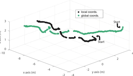
Figure 9. The path of a dragonfly along a pond shore, showing the raw points (black) and the path once the points have been transformed into global coordinates (green). The raw path appears shorter because the camera rig was rotated to follow the dragonfly, making the dragonfly appear to cover less distance than it truly did in global coordinates.
Between successive frames, the stationary point appeared to move on average 0.4 cm, with a standard deviation of 0.5 cm. Figure 11 shows the stationary point in 3D space before and after transformation into global coordinates. We then tested the rig in the field by filming dragonflies along the shore of a pond. Because dragonflies fly at a speed of about 3 to 7 m/s and should be traveling approximately 5 to 11 cm per frame, error of less than a centimeter per frame is not prohibitive for our purposes. We further confirmed that the algorithm was working by tracking several stationary points in dragonfly videos, and we found similar rates of error. We were able to rotate the rig to follow dragonflies along a longer
stretch of shore than could be seen in the cameras’ stationary frames. Fig. 6 shows a sample path of a dragonfly filmed while the rig was rotated to follow its flight. From these data, we were able to extract parameters such as velocity, centripetal force (measured in body weights), and relative headings of chased and chasing dragonflies.
Overall, the IMU rig worked and the concept seems sound, although there is still too much error for applications requiring high accuracy.
Future Work
The accuracy of the rig’s orientation could likely be improved by perfecting the Kalman filter and tuning it more precisely. Manual tuning of the constant multiplying the noise covariance matrix caused visible improvement; automated tuning or tuning based on more trials could make further improvement. There is little risk in overtraining the filter provided that sufficiently varied data is used.
More precise IMU instrumentation might also make a significant difference. Improvement might also be achieved by cross-referencing IMU data with tracked stationary points in each frame to get a better estimate of orientation; that is, using the IMU to get an estimate of orientation and then observing the observed rotation of stationary points in the video and using that as another method of estimating orientation.
Additionally, the stereo videography camera calibration had small inaccuracies that may have contributed significantly to the error. A more careful, precise camera calibration might improve accuracy of the entire set-up.
Acknowledgements
I would like to thank my advisor in Biology, Tyson Hedrick, for endless help and also for consistently excellent advice about what to Google; my advisor in Computer Science, Diane
Pozefsky, for all her help and for agreeing to take me on last minute; Jan-Michael Frahm for agreeing to be my second reader and for good suggestions about how to cut down on error in Version 2 of the DragonflyChaser3000XLE; and the Hedrick Lab for support and advice.
Funding was provided by a Taylor Fellowship from the UNC Chapel Hill Office for Undergraduate Research.
References
Abdel-Aziz, Y. I. (1971). Karara. HM (1971) Direct linear transformation from comparator coordinates into object-space coordinates in close-range photogrammetry.
In Proceedings ASP/VI Symp. On Close-Range Photogrammetry (pp. 1-17).
Clifton, G. T., Hedrick, T. L., & Biewener, A. A. (2015). Western and Clark's grebes use novel strategies for running on water. Journal of Experimental Biology, 218(8), 1235-1243. Gander, W., Golub, G. H., & Strebel, R. (1994). Least-squares fitting of circles and ellipses. BIT
Numerical Mathematics, 34(4), 558-578.
Hartley, R., & Zisserman, A. (2003). Multiple view geometry in computer vision. Cambridge university press.
Kress, D., Van Bokhorst, E., & Lentink, D. (2015). How lovebirds maneuver rapidly using super-fast head saccades and image feature stabilization. PloS one, 10(6), e0129287.
Leccadito, M., Bakker, T. M., Niu, R., & Klenke, R. H. (2015). A Kalman Filter Based Attitude Heading Reference System Using a Low Cost Inertial Measurement Unit. In AIAA
Guidance, Navigation, and Control Conference (p. 0604).
Munk, Y., Yanoviak, S. P., Koehl, M. A. R., & Dudley, R. (2015). The descent of ant: field-measured performance of gliding ants. Journal of Experimental Biology, 218(9), 1393-1401.
Schönberger, J. L., & Frahm, J. (2016). Pixelwise View Selection for Unstructured Multi-View Stereo. In European Conference on Computer Vision (ECCV).
Schönberger, J. L., & Frahm, J. (2016). Structure-from-Motion Revisited. In IEEE Conference on Computer Vision and Pattern Recognition.
Shelton, R. M., Jackson, B. E., & Hedrick, T. L. (2014). The mechanics and behavior of cliff swallows during tandem flights. Journal of Experimental Biology, 217(15), 2717-2725.
Sholtis, K. M., Shelton, R. M., & Hedrick, T. L. (2015). Field flight dynamics of hummingbirds during territory encroachment and defense. PloS one, 10(6), e0125659.
Shoemake, K. (1994). Euler angle conversion. Graphics gems IV, 222-229.