Acknowledgements
I would like to first thank my advisor, Professor David Guilkey, for all the help and
guidance that he has provided me throughout this process. With his wealth of econometric
knowledge and my lack thereof, I was able to deeply expand my understanding of econometrics
Thanks to Professor Guilkey’s patience and knowledge, I was also able to properly construct
each model and develop the methodology used to calculate my results. Without Professor
Guilkey’s guidance, this thesis would not have been completed.
I would also like to thank Dr. Klara Peter for guiding me and the whole class through the
completion of this thesis. She provided the framework in which research is conducted, and with
her guidance, I was able to remain on track throughout this entire process. Dr. Peter also forced
me to constantly expand my analysis further and to not be satisfied with the easiest approach.
I also want to thank my friend Andrew Castro for helping me with the data collection
process. Without his programming ability, the data collection process would have been
exponentially longer than it was, and the thesis would not have likely been completed within the
given time frame. Having him as a source for feedback also allowed me to think through
2
Abstract
In this paper, the NFL draft process at an individual and team level will be investigated
using multiple approaches. At the player level, this paper will seek to find which player level
characteristics have the most significant impact in determining where a player is to be picked and
how he performs in the NFL. With the inclusion of word characteristics from scouting reports,
the paper aims to approach the player analysis through combining both quantitative and
qualitative factors. A player level panel data set is constructed so that change in player
performance could be tracked over time. In addition to the individual player analysis, the paper
conducts a team level analysis that aims to determine the exact impact of player inputs separated
by position from both the offensive and defensive side of the ball. The paper will also explore the
impact that the drafting ability of teams on both sides of the ball have on their respective
performance. The use of player scouting reports and language processing in the context of
quantitative analysis has not been done in previous literature and will be the main contribution of
3 I. Background
Employers often make mistakes in determining the aptitude or qualifications of a
prospective employee. They go through extensive resumes, interviews, and background checks
to ensure that the candidate is qualified. The same process works for the NFL in their annual
player draft. What this paper aims to analyze are the specific traits in college players that are the
most significant for NFL success and the impact the accuracy of NFL decision makers has on
team performance.
The NFL draft is a system in which college players transition from college to different
NFL teams. It was first instituted in 1936 as a way to ensure competitive balance as Bert Bell,
the owner of the Philadelphia Eagles during the time, had complained to the league that the team
was not able to sell tickets to games because of market restrictions that prevented his team from
employing better talent. Under a completely open labor market, players signed with teams that
had better prestige or ability to win given the same amount of money. Since the Eagles were not
winning games, players would not sign with them, and then since the Eagles could not sign better
talent, they kept losing games (Lyons 2009).
To combat this unending cycle of losing, Bert Bell proposed that the league employ a
reverse-order player draft in order to improve competitive balance in the league and thus,
improve the profitability of the league. It was unanimously approved. The order of the draft was
determined by the win records for all the teams and various tie-breakers. The team with the most
losses was awarded the first pick out of a pool of college players determined by the league before
the draft. Currently, there are 7 rounds of the draft with a pick for each of the 32 teams, and
4
Ever since ESPN aired the draft on its network in 1980, its popularity among the general
public has increased tremendously. For what was once a private, closed-door event where media
coverage consisted of a list of players after the draft, the draft has now become a media bonanza.
Between ESPN and the NFL Network, there was an average of roughly 5 million viewers across
the three days the draft was held in 2016 (SportsBusinessJournal 2016). Moreover, the NFL has
worked to make the draft process a prolonged source of entertainment for fans from the end of
the season up to the draft. Pre-draft All-Star games such as the Senior Bowl and East-West
Shrine Bowl and the practices that precede them are now broadcast to the general public for their
consumption.
When selecting a player, the teams review all the available information on players from
their college performance, interviews with team officials, workouts, and background checks.
With the abundance of information, it is easy to get lost in the shuffle and lose sight of what
factors are actually important in predicting a player’s success in the pros. What this paper aims to
accomplish is to isolate these characteristics based on the information from scouting reports and
determine the predictive power of these characteristics on future NFL success.
With the large increase in popularity and abundance of information of the draft process
available to the general public, front office decision makers are under more scrutiny than ever
before, and criticism comes quickly anytime a highly-drafted player does not meet expectations.
However, in relative terms, front office decision makers are relatively good at
determining successful players.
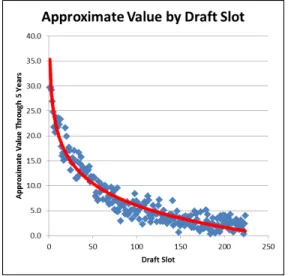
[INSERT FIGURE 1: Approximate Value by Draft Slot]
The above graph made by Chase Stuart of Football Perspective shows the relationship
5
deemed more valuable) and Approximate Value (AV) of a players’ first five seasons (a player
performance metric created by ProFootballReference to be discussed later on) from the 1980 draft
to the 2007 draft (Stuart 2012). Only the first five seasons of a player is counted because draft
picks have contract lengths of 5 years when they first enter the league. Therefore, in order to
calculate returns on investment for a team on a draft pick, it is best to only count the first five years.
In the graph, there is a clear relationship between how early a player was chosen and their
productivity in the league. This indicates that NFL decision makers are very capable of
determining which players are more likely to succeed and that the NFL on a macro level correctly
picks the better players earlier in the draft.
[INSERT FIGURE 2: Chance a Player is a Bust]
However, the rate of failure of these draft picks is still fairly large. Defining a bust to be a
player that starts for less than one year or plays less than 40 games in his career (in other words,
not a successful draft pick), the probability of picking a bust at the end of the 1st round (% Bust in
the graphic) is at around 30%, and at the end of the second round, the bust rate is about 50% (Wolf,
Malmgren, and Stringer, 2012). Pick number in this instance is the same as draft slot, and a lower
pick number indicates the player was picked earlier and was deemed more valuable.
There are several reasons to explain the relatively high failure rate of draft picks. Although
sheer randomness (injuries, off-the-field issues, player developmental aspects) plays a significant
factor in the bust rate, inherent biases within the decision makers could also be responsible. For
example, some NFL decision makers tend to prioritize height for quarterbacks. In the 2010 NFL
draft, many NFL scouts downgraded Wisconsin quarterback Russell Wilson solely because of his
height. At 5’11, he was much shorter than the NFL QB average of 6’4, and many decision makers
6
Despite Wilson being a tremendous quarterback prospect otherwise, many teams did not consider
him to be a starting caliber quarterback. Despite the fact that quarterbacks are in high demand in
the NFL and are routinely drafted higher than they should, he dropped to the third round and 75th
pick overall solely because of his height. Even though NFL decision makers are nearly certain that
height is an absolutely indispensable characteristic for an NFL quarterback, a study done by Berri
and Simmons in 2009 shows that for quarterbacks drafted from 1970 to 2007, there is no significant
relationship between height and quarterback performance in the NFL.
The height of quarterbacks is one example of many biases that exist in the NFL scouting
world. Many studies have been done to determine if performance metrics of college players have
any predictive power in determining their performance in the NFL, but they fail to account for the
variability of characteristics that cannot be captured numerically. The majority of these objective
metrics are collected in an event called the Combine, where players perform athletic tests such as
the 40-yard dash/sprint, vertical jump, bench press, and other drills that measure their physical
abilities. However, these drills are done in shorts and t-shirts and are not done in the context of an
actual football game. Therefore, the carryover of these measures onto actual football ability is
somewhat limited and do not account for specific football skills, such as reading a defense or
beating double teams.
What this study aims to accomplish is to set the framework for analyzing these football
specific characteristics by parsing scouting reports of NFL teams. In addition, the study aims to
determine characteristics NFL teams wrongly put too much focus on in their player evaluations,
such as height in quarterbacks, and how they affect team performance. This paper will also try to
find characteristics that have significant predictive ability of performance in the NFL. Because the
7
such as arm strength, pocket ability, and accuracy in college affect NFL performance. The study
will also contrast those characteristics to those that cause teams to draft players earlier than others.
Lastly, this paper will attempt to analyze the relationship between drafting accuracy and team
performance, controlling for the ability of the player inputs.
Overall, there are a few contributions that this paper will add to the existing literature. It
will be the first paper to introduce the concept of language processing and characteristic analysis
in the framework of sports and predicting player ability. The paper will also be one of the first to
analyze player production through time. Many studies have analyzed production for a player in an
absolute sense in context of a career, but this study will focus on production on a year to year basis.
The methods of this paper could also potentially be utilized in fields other than sports, where
scouting reports could be replaced by resumes and background checks. By using this methodology,
employers will be able to better identify what specific characteristics in an employee are important
in determining their future productivity in the workplace.
III. Literature Review
There have been several studies related to the topic at hand. As mentioned before, the
seminal study done by Cade Massey and Richard Thaler is “Overconfidence Vs. Market
Efficiency in The National Football League” (2005). This study focused on analyzing the actual
value of a draft pick in the market created by the decision makers and whether or not these
decision makers correctly assess the value of these draft picks by analyzing draft trades. Their
study finds that the market is actually not efficient and that in the first round, there is more value
to be acquired by picking later rather than earlier. They found that trading a high pick for several
8
reasons, such as psychological aspects, of possible biases of NFL decision makers. To measure
player performance, they have developed a metric based on the number of games played and
number of pro-bowl appearances (an All-Star game in the NFL). However, this metric might not
be the most accurate indicator of success because it is largely influenced by the decision makers
themselves. Decision makers, for the most part, decide who gets to play, and if they invested a
good deal of resources on a player, they would be more inclined to keep playing that player to
save face.In essence, Thaler and Massey use the decision-makers statements about the players to
explain the rationality of the decisions they have made on the said players. As stated before, this
study will try to account for this by using Approximate Value as the dependent variable instead
of the metrics that Massey and Thaler use. Despite this, the study is a good overview of the
value, or at least perceived value, of draft picks in the NFL.
The second study relates to player projections based on physical characteristics,
completed by Berri and Simmons called “Catching a draft: on the process of selecting
quarterbacks in the National Football League amateur draft” (2011). Berri and Simmons sought
to explore whether or not several physical characteristics affect NFL performance for college
quarterbacks. They used metrics like height, BMI, college performance, the Wonderlic (a test for
“intelligence” for college players), and other physical tests to conduct their analyses. They found
that while some metrics like height, Wonderlic, and speed can help predict which players will be
drafted higher, these same characteristics are not able to correctly predict the success of these
quarterbacks in the NFL. Compared to Thaler and Massey, Berri and Simmons use a variety of
metrics such as QB Rating, Wins Added, and Yards Added to assess the performance of these
QBs. They also found that although there is some evidence for scouting data explaining variation
9
measures in their analysis, the study is limited to only quarterbacks and does not include any
qualitative measures in their analysis.
In a third study, “Evaluating National Football League Draft Choices: The Passing
Game” completed by Boulier, Steckler, Coburn, and Rankins, the researchers approached
evaluating NFL decision makers in a similar manner to Thassey and Maler. The only slight
difference is that they consider the whole duration of the players’ careers instead of solely
focusing on their production to the team that drafted them. They also only study wide receivers
and quarterbacks. Moreover, they used Spearman’s Rank-Order correlation in order to compare
the position rank with which a player was drafted (whether a player was the first, second, third,
etc. quarterback or receiver taken) and their production, compared to the simple ordinary least
squares regression conducted by Berri and Simmons and Massey and Thaler. They concluded
that NFL decision makers can effectively rank players’ future performance relative to each other.
However, they ignore the individual characteristics of the players and simply look at their ranked
draft positions compared to other players of the same position to determine the success of
decision makers.
The limitation of this study is similar to that of Massey and Thaler, where a players’
performance is calculated through games played and other longevity measures. Because Boulier
et al. are conducting assessments of players across their whole careers, games played and other
longevity measures are more suitable for determining a players’ success than Massey and
Thaler’s study, where they only take into consideration the player’s first five years. However,
there can still be bias in the data as the players taken higher up in the draft will be given more
10
Another relevant study is an exploration of the relationship of draft pick value and its
effect on improving team quality. In “Deconstructing the Draft, An Evaluation of the NFL Draft
as a Predictor of Team Success,” Bonds, LeCrom, Reynolds, and Thompson sought to determine
whether or not the NFL draft is a good form of establishing competitive balance in the league.
Competitive balance is defined as equal quality of teams across the league over time so that one
team does not either perform poorly or dominate over a long period of time. The researchers
used “the Chart” (a relatively arbitrary draft value board created in the 1990s) to assign value to
the draft picks teams had in a given draft and then measured the change in winning percentage
that resulted from the total value accumulated. They have determined that there is a significant
positive correlation between the total draft value and change in winning percentage. The teams
with higher positioned draft picks and a higher number of draft picks did win more games the
following season compared to teams with lower positioned draft picks, which is a good indicator
that the quality of drafts do impact winning percentage and that the draft in general promotes
competitive balance.
There are some limitations to the study. For one, it does not factor into its calculations the
impact that free agency has on team quality. A team might have a low level of talent employed
and thus plenty of cap space (or amount of money to spend) to sign more talent the following
season. Another limitation is that the study does not account for the other measures that the NFL
takes to ensure competitive balance. The most glaring that the study ignores is the scheduling of
the games. The league in its current form, with the expansion of the Houston Texans in 2002,
constructs the schedules of teams so that the weaker teams play more games against other
weaker teams and the performing teams will play more games against other
11
of team quality from the previous season. On the surface, 3 might not seem enough to cause a
significant impact, but due to the brevity of the NFL season of 16 games, those 3 games account
for almost 20% of the season.
IV. Data
In terms of the data, this study is concerned with players from the 2008 to 2013 NFL
drafts. This set of drafts has been selected because scouting and draft player analysis had not
been popularized before 2008. There are scarce scouting reports and complete sets of physical
characteristics online before 2008. The 2014-2016 drafts have been excluded because a sizable
sample of games played in the NFL is needed to properly assess whether or not the player is
successful. The 2013 NFL draft has four seasons worth of playing data, which is around the
minimum amount needed. Each player in the data set has information about the college they
attended, their associated conference and division, position, the team that drafted them, the round
drafted/overall pick number where they were drafted, the average Approximate Value (AV)
accumulated per draft slot, , height, weight, hand size, arm length, Wonderlic score, 40 yard
dash, 10 yard split, bench press, broad jump, shuttle time, 3 cone time, and games played/started,
pro bowls, all pro selections, AV for the 2008 through 2016 seasons, and word characteristic
dummy variables that have been parsed through scouting reports. All physical characteristics and
AV/NFL performance numbers have been taken from http://nfldraftscout.com/,
http://www.pro-football-reference.com, http://nflcombineresults.com, and http://nfl.com.
General Statistics
Approximate Value (AV) is a metric created by ProFootballReference that assesses the
relative quality of a player. The creator of the metric states that the metric is not supposed to be
12
but it is an improvement on metrics such as “number of seasons as a starter” or “number of times
making the pro bowl.” The metric was modeled after the Value Approximation Method used by
baseball analysis pioneer Bill James in comparing the relative quality of players’ seasons. The
goal of the metric was not to be a definitive guide in saying which players were better, but rather
that a group of players with a higher AV was better than a group with a lower AV. As put by the
creator of the metric, Doug Drinen: “Again remember that the goal here is not to forever put an
end to the debate about whether Daniel Graham or Antonio Bryant has had the better career.
That’s too ambitious a goal. We simply want to classify them both as being a bit better than
Michael Bishop or Travis Dorsch, but not as good as Terry Glenn or Carson Palmer.” The metric
is created by divvying up a pool of points, which is determined by points scored/allowed on
offense defense, to each position weighted by metrics created by Drinen that relatively
proportion out the importance of each position based on yardage created by each individual
position group (Described further by Drinen in his website). Then the divvyed up points are
weighted by individual performance measures such as throwing yards, touchdowns, tackles,
interceptions, sacks, etc. An interested reader can refer to Drinen’s website listed at the end of
the paper (Drinen 2008). All in all, AV serves as the best available dependent variable to
measure the value a player provides to his team. Modern NFL data analytics sites such as
FiveThirtyEight and Football Perspective rely on Approximate Value heavily.
As mentioned previously, the average AV accrued per draft pick was formulated by
Chase Stuart of Football Perspective, where for each draft slot, he calculated the average
Approximate Value accumulated by the player’s first five seasons. He then fitted the values into
13
players and the expected value of performance per draft pick is quantified by AV, you can
directly compare the two values. Only the first five years of a draft pick is used because
five years is the length of the first contract the player receives upon entering the league. More
often than not, the player spends five years with their first team before they decide to stay with
their current team or leave via free agency. Using the AV of the first five years is a good
indicator of how much value a draft pick contributed to the team on average.
Below are summary statistics of the Height, Weight, 40 Yard Dash Times, and Total
Approximate Value accumulated over a player’s career:
[INSERT TABLE 1: Player Summary Statistics]
[INSERT TABLE 2: Player Summary Statistics Across Years]
The tables above show the summaries of the tangible player data measured at the
Combine or Pro Day from 2008 to 2013. The average height in inches for a player from the 2008
to 2013 draft is close to 74 inches or 6’2”; the average weight is near 243 pounds; the average
time it takes for a player to run 40 yards is approximately 4.827; and the average total
Approximate Value (total amount of production from a player over their career) is 2.115. In our
sample of seasons from 2008-2016, the minimum AV in a given season was -5, and the
maximum was 22. Table 2 divides the group of players by what draft class they were from, and it
can be seen that the measures are all similar across years.
In terms of the team data, season data of teams are collected from 2008 to 2016 and
consist of Total Defensed-adjusted Value Over Average Percentage (Total DVOA%), Defensive
DVOA% (DDVOA%), Offensive DVOA% (ODVOA%). DVOA is a metric calculated by
Football Outsiders that “measures a team’s efficiency by comparing success on every single play
14
accumulate the success rate of all plays on both offense and defense into a cumulative metric that
outlines performance on both sides of the ball.
Table 3 outlines the average approximate value assigned to each position for each time while
Table 4 outlines the summary statistics of the team measures listed above.
[INSERT TABLE 3: Team AV Summary Statistics]
[INSERT TABLE 4: Team Summary Statistics Across Years]
Both the individual and team models to be introduced later on in the paper are organized
as panels. Panel data is a combination of both cross-sectional data and time-series data.
Cross-sectional data consist of a sample of individuals, households, firms, etc. taken at any point in time
(Wooldridge, 2012), and time-series data consist of variables or several variables observed over a
period of time. Examples include GDP, stock prices, CPI, and crime rates. Putting them both
together, panel data consist of samples of individuals, households, and firms observed over a
period of time. Instead of just one cross-section, it is multiple across many years. The firms in the
context of this paper are either the individual player or the teams, and their respective information
will be recorded across time. As stated before, the sample of players are from the 2008-2013 drafts,
and their playing data is recorded from 2008-2016. Likewise, the team performance data is
recorded from 2008-2016.
Word Analysis of Scouting Reports
With regards to scouting report data, they have all been acquired through either
NFL.com’s or cbssports.com’s combine section, where nearly every player invited to the
combine was assessed by their independent experts with an accompanying scouting report.
Selection bias is a possible issue because only players with scouting reports are included in the
15
players to limit this. However, we do admit that the lack of a large number and variety of the
scouting reports are a limitation of this study.
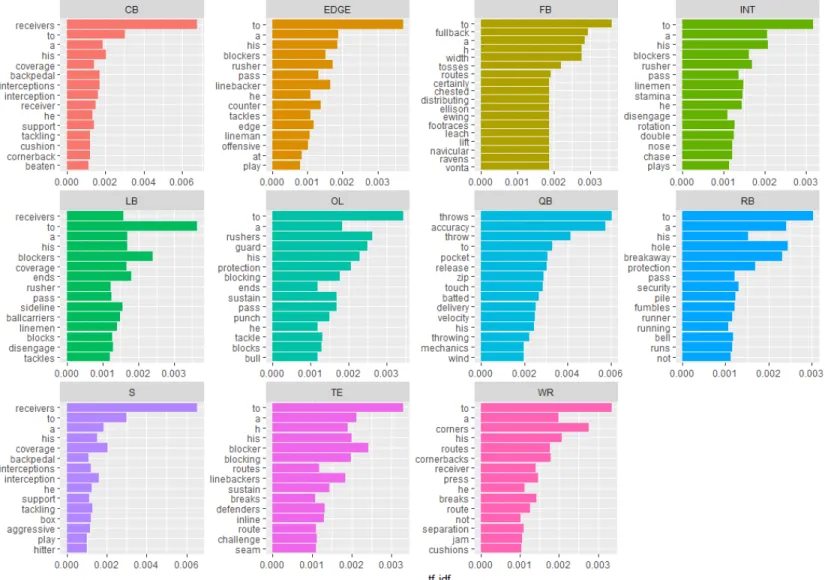
The scouting reports have been analyzed using a text-mining concept called tf-idf or term
frequency-inverse document frequency. It is a method to determine which words or
characteristics are important or significant, and tf-idf is the product of both term-frequency and
inverse document frequency. Term-frequency is the log of the raw number of times a word
appears in a given document with a Boolean of whether or not the word appears in the document
to weight the term in the document, which is a subset of a collective corpus (Mogotsi, 2009). In
this case, the document is one individual scouting report, and the corpus is the entire collection
of scouting reports. Inverse document frequency is calculated by determining how often a word
appears throughout all the documents. For example, the word “the” will appear in nearly all if
not all of the documents and thus will be weighted very low on the idf scale. In the context of
this study, there are two sections with strengths and weaknesses of each player in each individual
scouting report. To account for negative words and to allow for ease of analysis, the scouting
reports are split into two corpuses of strengths and weaknesses for all the players. Then separate
analysis is conducted to see which words are the most important in both strengths and
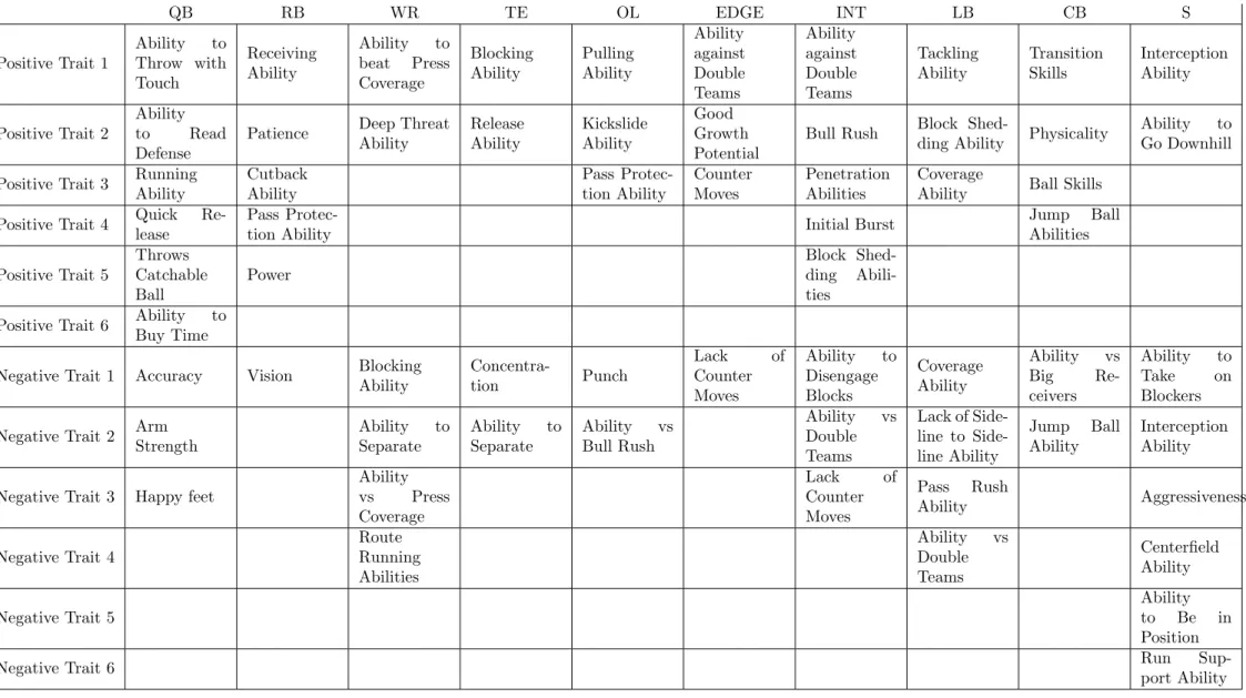
weaknesses. To parse important characteristics of each position, words and their tf-idf scales are
ranked by position to see which words are the most important in each position. The top 15 words
by position for both strengths and weaknesses are shown below.
[INSERT FIGURE 3: Strengths Unigrams by Position]
[INSERT FIGURE 4: Weaknesses Unigrams by Position]
Then specific words from each position are picked because of their corresponding player
16
these characteristics. For example, “motor” for an EDGE player indicates high effort in nearly all
circumstances.
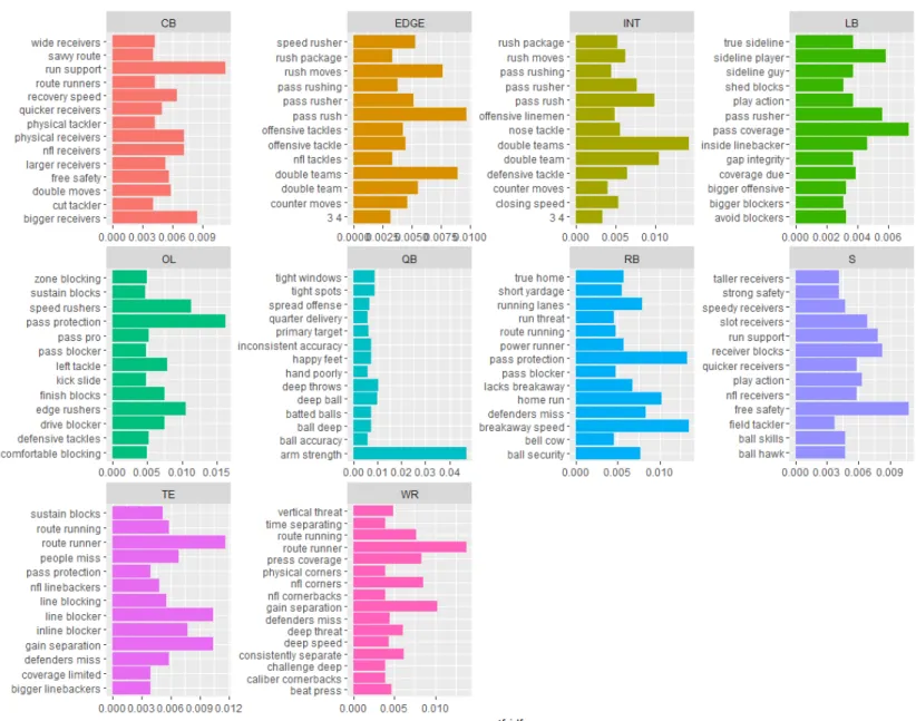
This same approach can be applied to what are called bigrams, or simply a phrase
consisting of any two words. Because of the simplicity of single words, extending the analysis to
bigrams allows for more specific characteristics to be drawn from the scouting reports. The
corresponding charts are displayed below.
[INSERT FIGURE 5: Strengths Bigrams by Position]
[INSERT FIGURE 6: Weaknesses Bigrams by Position]
Characteristics were then chosen from the top 15 unigrams and bigrams listed above. For
each chosen characteristic, a corresponding dummy variable was created for each report that
indicates that the report contains the characteristic.
There is however a limitation with this word analysis that largely stems from the fact that
while these analysts are employed by the NFL, they are just media people and not professional
scouts who are trained and well versed in scouting characteristics. In this dataset of scouting
reports, the evaluations of the offensive line in particular are somewhat limited and lacks the
terminology and breadth of words utilized in other positions. Because of this, the specificity and
depth of offensive line characteristics are not the same as those from other positions. This paper
will simply admit this shortcoming as a limitation of available data and assume that these
scouting reports are accurate.
Another limitation of this study is the grouping of positions. While there might be some
significant differences in the skillset required for a 1-technique nose tackle and a 3-gap
penetrating defensive tackle, these two positions will be grouped together as interior defensive
17
outside linebackers. Due to the limitations of sample size and lack of positional designation data,
this study will group together relatively similar positions.
A possible cause of bias in the data is that players drafted higher will have longer reports
than those who were drafted lower because the media focuses more on the better players who
would go earlier in the draft and who will likely draw more attention from the casual fan. To
control for this, we will include the pick number of the player as a proxy for report length in our
models. To ensure that pick number is an appropriate proxy variable, Pearson’s product-moment
correlation test was used to test the association between the length of the scouting reports and the
pick number of a player. The correlation coefficient is -.1529 and the t-statistic is -5.793, which
means that we reject the null hypothesis that the correlation between scouting report length and
the pick number of a player is 0. This means that pick number is a suitable proxy variable for
scouting report length.
IV. Theoretical Model
For the theoretical model, the paper will specify a team production function model with
player production along other factors to see which positions have the greatest impact on team
output. Speaking in a microeconomic sense, the main goal of any corporation or firm is to turn
inputs to outputs. In producing any output, whether it is cars, chocolate, airplanes, or clothes,
there are two essential components involved: capital and labor (Nicholson and Snyder, 2011).
Capital represents any raw materials or machines used to create the output, and the labor
represents people’s work used to combine, use, or transform the capital into the finished output.
In the context of this study, the firms are the 32 teams in the NFL, and their output is
18
facilities, stadiums, and other sorts of equipment. In our study, we assume that capital is fixed
and equal across all 32 teams because they all have roughly the same footballs, practice facilities,
stadiums, and equipment. The labor here is the level of play the players provide from different
positions, which combine to produce the output of team performance.
One could argue that managerial ability could be an important input that affects team
productivity (or output). In our models, to account for management ability of the teams, a proxy
variable of draft ability is used. It is calculated by summing up all the yearly differences of
expected return and actual output across positions for every draft class. This statistic includes the
differences for both offense and defense for two reasons. One, if the draft ability were to be
parsed into both offense and defense, the correlation between draft ability and the sample player
AV would be higher and cause higher standard errors. Second, using the cumulative version of
the statistic would be a better representation of the overall competence of the team. Because the
variable in question is proxying for overall management ability instead of management ability by
both offense and defense, it is best to use the composite statistic.
The models will be separated between offense and defense. Although one could argue
that defensive output could affect offensive output and vice versa (time of possession could be an
example of this), it is difficult to say that, within the context of the models, having more talented
cornerbacks or linebackers will improve output of the offense. The distribution of talent amongst
position from one side of the ball is very unlikely to affect the production of the other side of the
ball. With that in mind, the dependent variables for our models will be offensive DVOA% and
defensive DVOA%, which, as mentioned before, are opponent adjusted per-play efficiency. In
other words, the metric measures how effective an offense or defense is in a given play
19
Subsequently, a Cobb-Douglas might seem appropriate here as a specification of the
production function with DVOA as the output and the individual AV’s as the labor inputs with
no or constant capital across teams. A justification of this function form is that the value of one
group being exorbitantly high cannot compensate for a non-existent value of another group. For
example, an offense cannot have 11 offensive linemen and succeed without any of the other
parts. However, in this case, it is possible for a player to have 0 output in AV, so that situation
does not apply. While this approach does have theoretical merit, there is some mathematical
difficulty of incorporating drafting ability of teams in the estimation of the model as it cannot
equal to 0 because logs of 0 cannot be computed. Thus, the best way to compute the draft ability
of the teams is to measure the % return on investment. If a team invested 20 points into a running
back and received 12 points, then the %ROI is 60% (%ROI is not calculated the same as it
typically is in finance to avoid negative values).
There are two problems with this approach. One is that the measure does not account for
the amount of resources a team invests in a player. A team investing 40 AV and receiving only
10 AV has a larger measurable effect than one investing 4 AV and receiving only 1 AV, but the
measurement of return would be the same. Another issue is players accumulating 0 AV, which
cannot be transformed through a natural log. A way to combat this is to add a small number (.001
in this case) to all the AV. However, after the log, the results close to 0 will be heavily skewed
negatively more so than the positive values, which could distort the results.
V. Empirical Team Level Model
The data will be set in panel form with i being one of the 32 teams in the NFL and t being
20
input, a sample player AV input, and a draft ability variable. Sample player AV indicates AV
generated by the players in the dataset who were drafted from 2008 to 2013. Later, the choice
between fixed and random effects will be determined by whether or not player inputs are
correlated with “alpha.” To be discussed in the subsequent sections, there is reason to believe
that this correlation exists with the team models but not the individual models.
𝑂𝐷𝑉𝑂𝐴𝑖𝑡 = ∑5𝑗=1𝛽𝑗𝑛𝑜𝑛𝑠𝑎𝑚𝑝𝑙𝑒_𝑝𝑜𝑠𝑗𝑖𝑡+ ∑5𝑗=1𝛾𝑗𝑠𝑎𝑚𝑝𝑙𝑒_𝑝𝑜𝑠𝑗𝑖𝑡+ 𝛿1𝑑𝑟𝑎𝑓𝑡𝑎𝑏𝑖𝑙𝑖𝑡 + 𝛼𝑖+ 𝜖𝑖𝑡 (1)
𝐷𝐷𝑉𝑂𝐴𝑖𝑡 = ∑5𝑗=1𝛽𝑗𝑛𝑜𝑛𝑠𝑎𝑚𝑝𝑙𝑒_𝑝𝑜𝑠𝑗𝑖𝑡+ ∑5𝑗=1𝛾𝑗𝑠𝑎𝑚𝑝𝑙𝑒_𝑝𝑜𝑠𝑗𝑖𝑡+ 𝛿1𝑑𝑟𝑎𝑓𝑡𝑎𝑏𝑖𝑙𝑖𝑡+ 𝛼𝑖+ 𝜖𝑖𝑡 (2)
Here, ODVOA corresponds to the offensive DVOA% of team i in year t. The summation
for nonsample_pos represents the approximate value accumulated by each position j for team i in
year t for all players that are not included in the sample of players from 2008-2013. The
summation for sample_pos, in turn, represents the approximate value accumulated by each
position j for team i in year t for players included in the 2008-2013 sample. In addition, the alpha
term corresponds with the time-invariant error term, and the epsilon denotes the idiosyncratic
error. The time-invariant error term here would be referring to the team specific error term, or in
other words, unaccounted factors that affect performance that do not vary over time and are
specific to each team. The idiosyncratic error is not restricted to just the teams, and it represents
unobserved time-varying factors that affect performance. The DDVOA model is identical to the
ODVOA version except the dependent variable is defensive DVOA% and the positions
correspond to the defensive side of the ball.
VI. Empirical Player Level Model
The player level empirical model will deal with determining how various attributes, such
21
how high a team will draft a player and their performance in the pros. We will look at several
different models that consider both the larger overall pool of players irrespective of position and
position-specific models that delve into which position-specific characteristics are important
when determining the future success of a player.
Expected Return Models
First, we will look at models concerning draft position, and what characteristics will lead
NFL decision makers to pick a player higher up in the draft. There will be separate models for
both the overall pool of players and players separated by position. Simple OLS will be used with
expected return of the draft pick as the dependent variable. The expected return of the draft pick
is the average approximate value accumulated in the first five years in the league for each draft
slots. For example, the 1st overall pick, on average, has accumulated 43.2 AV in their first five
seasons. As mentioned earlier, these corresponding numbers have been taken from the work of
Chase Stuart from Football Perspective with a couple alterations. 3.6 AV was added back to each
draft slot, which Stuart subtracted in his formulation because he was analyzing marginal value of
drafted players against undrafted players. The lowest pick in his analysis was 224 with the
corresponding value of 3.7 (after adding back the 3.6) despite the fact that most modern drafts
now have in total around 255 picks. To account for this, I fitted a log function with the given
values from Stuart (as did Stuart from the career AV data) and extended the values to pick 256,
which is the lowest draft pick of all the drafts in the sample. Pick 256 corresponded to 2.6 AV.
Because the undrafted players are a part of the sample that is used during our analyses,
the undrafted players needed a corresponding expected AV as well. The figure had to be lower
22
successful undrafted players to pull the average above 0. Thus, all the undrafted players were
assigned an expected AV of 1, fitting both to the criteria above and that of simplicity.
𝐸𝑅𝑒𝑡𝑢𝑟𝑛𝑖= 𝛼0+ 𝛼1𝑁𝑃5𝐹𝐵𝑆𝑖+ 𝛼2𝐹𝐶𝑆𝑖+ 𝛼3𝐷𝐼𝐼𝑖+ 𝛼4 𝑂𝑡ℎ𝑒𝑟𝑖+ 𝛼5𝑈𝑛𝑑𝑟𝑎𝑓𝑡𝑒𝑑𝑖+ ∑9𝑝 =1𝛽𝑝𝑃𝑜𝑠𝑖𝑝+ 𝑢𝑖 (3)
The above model is for the overall player pool irrespective of position for player i. The
dependent variable here is the Expected Return for a player given his draft position. NP5FBS,
FCS, DII, and Other are dummy variables indicating the divisions of the colleges that the players
played in with the Power 5 group (a group of colleges consisting of the Big Ten, Big 12, ACC,
SEC, and the Pac-12, where the best players usually go to school) acting as the reference
category. Undrafted is another dummy variable that indicates whether or not a player was
drafted, and Pos reflects dummies based on the 10 positions of both offense and defense
(quarterback, running back, wide receiver, tight end, offensive lineman, edge defender, interior
defender, linebacker, cornerback, and safety).
𝐸𝑅𝑒𝑡𝑢𝑟𝑛𝑖𝑝= 𝛼𝑝+ ∑ 𝛽𝑝𝑗𝑐ℎ𝑎𝑟𝑖𝑝𝑗 𝑛
𝑗=1
+ ∑ 𝛿𝑝𝑘𝑝ℎ𝑦𝑠𝑖𝑝𝑘 𝑛
𝑘=1
+ 𝛾𝑝 𝑈𝑛𝑑𝑟𝑎𝑓𝑡𝑒𝑑𝑖𝑝+ 𝑢𝑖𝑝 (4)
Here, the overall pool of players is split based on position groups. The model now
introduces position-specific characteristics, char in the above equation, from the word analysis
and physical characteristics specific to player i at each position p. The number of characteristics
vary depending on each position, and the models only include characteristics that have a t
statistic greater than 1 in absolute value. The physical characteristics, phys in the model, also
vary upon position because some physical characteristics might be more important for some
positions but not for others. For example, while the bench press might be an integral measure of
23
undrafted dummy is the same as that from the overall model. The specification of word
characteristics and physical characteristics by position can be found in the tables for the models.
Probit Models
In order to estimate the players’ likelihood of playing a game in the NFL and the
likelihood of producing significant outputs, simple probit models at both the overall level and
position-specific level are implemented. Starting with the overall models:
𝑃𝑙𝑎𝑦𝑒𝑑∗= 𝛼
0+ 𝛼1𝑁𝑃5𝐹𝐵𝑆 + 𝛼2𝐹𝐶𝑆 + 𝛼3𝐷𝐼𝐼 + 𝛼4 𝑂𝑡ℎ𝑒𝑟 + 𝛼5𝑈𝑛𝑑𝑟𝑎𝑓𝑡𝑒𝑑 + ∑9𝑖 =1𝛽𝑖𝑃𝑜𝑠𝑖+ 𝑢 (5) 𝑃𝑙𝑎𝑦𝑒𝑑 = {1
0
𝑖𝑓 𝑃𝑙𝑎𝑦𝑒𝑑∗ > 0 𝑜𝑡ℎ𝑒𝑟𝑤𝑖𝑠𝑒
Played is a dummy variable indicating whether a player has appeared in at least one game
in his career. This model is identical to the previous Expected Return model for the overall
player pool aside from the new dependent value for the probability that a player played in the
league.
𝑃𝑟𝑜𝑑𝑢𝑐𝑒𝑑∗= 𝛼
0+ 𝛼1𝑁𝑃5𝐹𝐵𝑆 + 𝛼2𝐹𝐶𝑆 + 𝛼3𝐷𝐼𝐼 + 𝛼4 𝑂𝑡ℎ𝑒𝑟 + 𝛼5𝑈𝑛𝑑𝑟𝑎𝑓𝑡𝑒𝑑 + ∑9𝑖 =1𝛽𝑖𝑃𝑜𝑠𝑖+ 𝑢 (6) 𝑃𝑟𝑜𝑑𝑢𝑐𝑒𝑑 = {1
0
𝑖𝑓 𝑃𝑟𝑜𝑑𝑢𝑐𝑒𝑑∗ > 0 𝑜𝑡ℎ𝑒𝑟𝑤𝑖𝑠𝑒
The model for whether or not a player has produced is identical aside from the dependent
variable. Produced is a dummy variable that indicates whether or not a player has produced more
than 3 AV at any point in his career. This is because 3 points is right around the cutoff for
significant production on either defense or offense for AV. For both the Played and Produced
models, physical characteristics were excluded because of the wide variance of these physical
24
lineman could run a 5.3 40-yard dash. Because of this wide variability, the physical
characteristics lose meaning within the overall player pool.
For the player specific models:
𝑃𝑙𝑎𝑦𝑒𝑑𝑝∗ = 𝛼0+ ∑ 𝛽𝑖𝑗𝑐ℎ𝑎𝑟𝑝𝑗 𝑛
𝑗=1
+ ∑ 𝛿𝑖𝑘𝑝ℎ𝑦𝑠𝑝𝑘 𝑛
𝑘=1
+ 𝛾𝑝 𝑈𝑛𝑑𝑟𝑎𝑓𝑡𝑒𝑑𝑝+ 𝑢𝑝 (7)
𝑃𝑙𝑎𝑦𝑒𝑑 = {1 0
𝑖𝑓 𝑃𝑙𝑎𝑦𝑒𝑑∗ > 0 𝑜𝑡ℎ𝑒𝑟𝑤𝑖𝑠𝑒
The Played variable is the same as the position-specific Expected Return model except
that the dependent variable is now the probability a player played in the NFL. In addition, the
specific characteristics of significance might be different from that of the Expected Return
models, and the physical characteristics are also again different by each position.
𝑃𝑟𝑜𝑑𝑢𝑐𝑒𝑑∗𝑝= 𝛼0+ ∑𝑛𝑗=1𝛽𝑝𝑗𝑐ℎ𝑎𝑟𝑝𝑗+ ∑𝑛𝑘=1𝛿𝑝𝑘𝑝ℎ𝑦𝑠𝑝𝑘+ 𝛾𝑝 𝑈𝑛𝑑𝑟𝑎𝑓𝑡𝑒𝑑𝑝+ 𝑢𝑝 (8)
𝑃𝑟𝑜𝑑𝑢𝑐𝑒𝑑 = {1 0
𝑖𝑓 𝑃𝑙𝑎𝑦𝑒𝑑∗ > 0 𝑜𝑡ℎ𝑒𝑟𝑤𝑖𝑠𝑒
The Produced model is largely the same as the Played model with the only difference
being the dependent variable. There is some variation in the significance of the word
characteristics as those significant in the played model might not be significant in the produced
model and vice versa. The differences in characteristics that are significant in the played model
but not in the produced model (or vice versa) could glean insight into which characteristics are
important for playing in the league versus contributing in the league.
Approximate Value Panel Model
To determine various individual characteristics’ effect on AV over time, panel data
25
to analyze the trajectory of a player’s performance over their first few years. The data is
structured so that for every season a player has participated in the league, he has one observation.
In addition, like the previous models, both the overall player pools and the individual position
models will be estimated. In regards to the time invariant error in the individual models, one
could make an argument that the effect is not correlated with the other regressors. Factors such
as intelligence and circumstantial characteristics (upbringing, access to resources, etc.) could be
included in the individual player effect, and one could argue that they would not correlate highly
with the regressors included in the models. For example, intelligence is not very likely to be
correlated with the number of reps in the bench press. Subsequently, one could argue that
compared to the team models, where the teams get to choose their individual player inputs which
increases the likelihood of endogeneity, the player’s models are more likely to have no
correlation between their regressors and the time-invariant error. In addition, many of the
physical characteristics included in the model are time-invariant as they were recorded right
before the player enter the league. If a fixed effects model were to be used, then these
time-invariant regressors would be differenced out and not included in the model. Because of these
reasons, a random effects model will be specified.
𝐴𝑉𝑖𝑡 = ∑ 𝛽𝑗𝑦𝑒𝑎𝑟𝑖𝑡𝑗 8
𝑗=1
+ 𝛿1exp𝑖𝑡+ 𝛿2exp𝑖𝑡2 + ∑ 𝛾𝑘𝑑𝑖𝑣𝑖𝑠𝑖𝑜𝑛𝑖𝑘 4
𝑘=1
+ 𝜌1𝑈𝑛𝑑𝑟𝑎𝑓𝑡𝑒𝑑𝑖+ 𝛼𝑖+ 𝜖𝑖𝑡 (9)
AV is approximate value for an individual player i in a given year t. The summation of
year is a series of dummy variables that correspond with the year of the season to account for
variation of AV in a given year. The exp and exp2 variables correspond with experience to
control for whether a player’s experience affects his AV and experience squared to allow for the
26
ability from his first year to his second year rather than going from his 10th year to his 11th year.
The summation of division is a collection of time-invariant dummy variables for college division
similar to those of the previous models. Undrafted is another time-invariant dummy variable that
delineates whether or not a player is drafted. The alpha term is the time-invariant error term, and
the epsilon corresponds with the idiosyncratic error. As mentioned before, the time-invariant
error term represents individual specific factors that are not observed by the model that affect
performance. In this case, it could represent factors such as mental toughness, childhood
upbringing, access to resources, and other various factors that are specific to the individual. On
the other hand, idiosyncratic error term refers to unobserved factors that do change over time.
𝐴𝑉𝑝𝑖𝑡= ∑ 𝛽𝑝𝑗𝑐ℎ𝑎𝑟𝑝𝑗𝑖 𝑛
𝑗=1
+ ∑ 𝛿𝑝𝑘𝑝ℎ𝑦𝑠𝑝𝑘𝑖 𝑛
𝑘=1
+ 𝛾𝑝 𝑈𝑛𝑑𝑟𝑎𝑓𝑡𝑒𝑑𝑝𝑖+ 𝛿1exp𝑖𝑡+ 𝛿2exp𝑖𝑡2 + 𝛼𝑝𝑖+ 𝜖𝑝𝑖𝑡 (10)
This model is again similar to the previous model except the player pools are grouped by
position and the position-specific word characteristics (denoted above by char) and physical
characteristics (denoted by phys) are introduced into the model. As stated previously, because of
the high likelihood of there being no correlation between the individual player effects (denoted
by alpha in the above equation) and the regressors, a random effects model will be utilized. The
division dummy variables will also be left out due to limited degrees of freedom.
VI. Results and Findings
Individual Player Models Results
Starting with the expected return models, we look at the players in the overall pool for the
two groups, one including both undrafted and drafted players and one including just drafted
players.
27
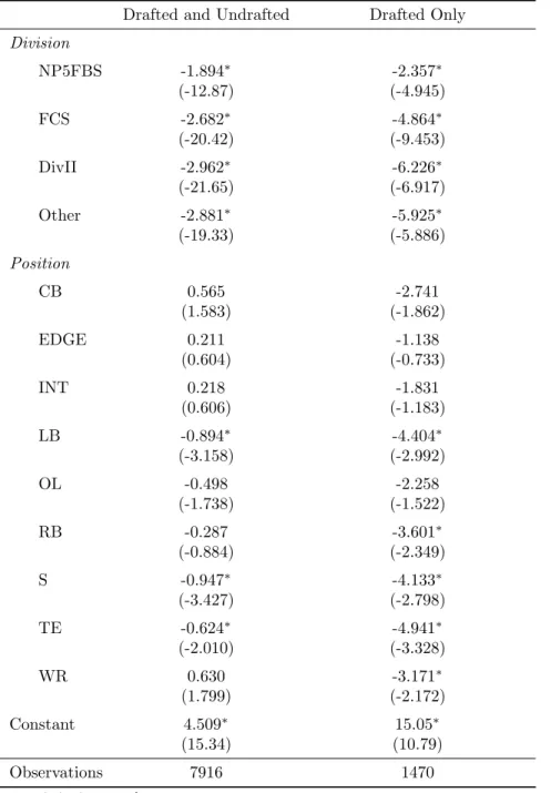
[INSERT TABLE 6: Positional Expected Return Regressions]
The results for both of these models are close to what you would expect based on the
current beliefs of the NFL. With the division dummies, the base group here is the Power 5
conference, which is the best division in college football. Because they have the best players, all
the other division dummies are negative and significant for both models. The Non-Power 5 FBS
division is the second-best division, and as expected, they come in second for both models
followed by the FCS division. After the FCS, the talent level is very sparse and uniform across
the board, so the Division II and the Other division dummies (Other including various small
divisions such as HBCUs, Division III, etc.) are relatively similar with the Other division having
slightly higher expected return.
Looking at the positional dummies, it is interesting to see how NFL teams value different
positions. In the model including both drafted and undrafted players, only linebackers, safeties,
and tight ends are valued significantly less than quarterbacks. In the model including only
drafted players, wide receivers and running backs are included in this group as well. While there
are some positive coefficients in the model including both (that are not significant), they all turn
negative as soon as the sample is limited to drafted players, which reinforces current mainstream
thought of the quarterback being the most valued position. This discrepancy might arise because
of the abundance of mediocre quarterbacks in the drafted and undrafted model. Between the
drafted model and the drafted and undrafted model, there might be a very large supply of
quarterbacks in the latter, but a vast majority of which that are not NFL-caliber. Therefore, they
could as a whole depress the value of quarterbacks in the undrafted and drafted model.
Because of the possibility of a high supply of mediocre talent, it will be best to look at
28
truly values in the league. In terms of positional value, quarterbacks are the highest as stated
before, and edge defenders and interior defenders come second and third respectively. This is an
interesting but also expected result because it reflects the belief that because the quarterback is
the most important, the people that come next in importance are the ones that affect the
quarterback’s play. In the eyes of the NFL, edge defenders and interior defenders have the
highest impact on quarterback play because any amount of pressure they generate will hinder the
quarterback’s the most. Predictably, the next group in order of importance is offensive linemen,
players that protect the quarterback against these defenders.
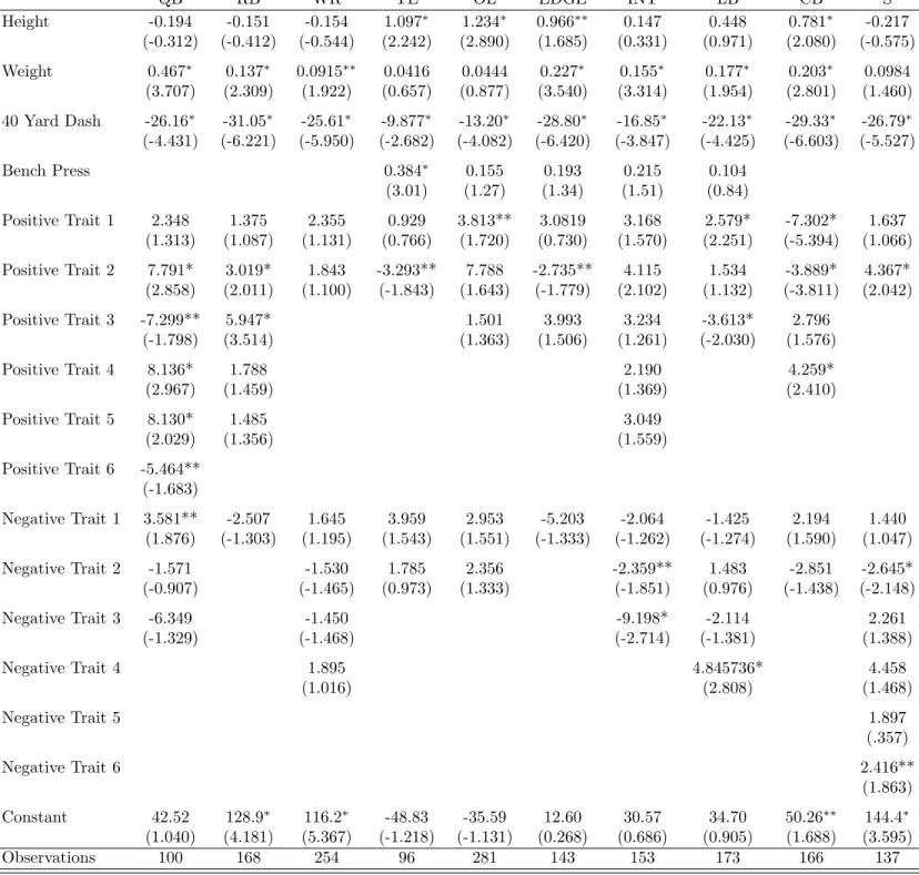
Next, we will look at the positional breakdown of expected return to see which
characteristics NFL decision makers value in drafting a player. However, as there are 10 position
groups, this paper, will focus on the quarterbacks for the sake of brevity, instead of going
through an extensive explanation for each position. All the regressions and their respective
position-specific characteristics will be listed at the end of the paper for the interested reader.
[INSERT TABLE 6: Positional Expected Return Regressions]
[INSERT TABLE 7: Corresponding Characteristics for Table 6]
In these models, due to the limited sample size, we will consider models at a 10%
significance level or at a 1.65 t-statistic. Here, in the quarterback model, we see that the most
important traits that NFL decision makers look for are a quick release and the ability to throw
catchable balls. It seems as the significance of these two variables show that the easy and visible
aesthetic qualities of a quarterback, such as how fast they release the football or the way the ball
looks coming out of their hand, play a significant role in how they are evaluated. That is not to
say that these decision makers complete ignore other facets of the quarterback, but that these
29
regression is the quarterback’s ability to read a defense, which shows that the intelligence of a
quarterback is important as well in NFL decision makers’ evaluations.
The interesting negative dummy variables in this case are the running and buy time
dummy variables. These variables largely represent traits that signify a quarterback who plays
out of structure and relies more on their running ability than staying in the pocket and making
throws. With the archetypical view of the pocket quarterback that is embedded within the NFL,
quarterbacks who stay in the pocket and operate from the pocket are more in demand than those
who run more than they throw and try to escape the pocket at any opportunity. Moreover, while
not significant at the 10% level, the dummy variable for happy feet, which is also another trait
indicating a quarterback’s lack of comfort from within the pocket, is also negative, which
supports the above conclusions.
Lastly, the interesting and sort of contradictory result from the above regression is the
positive sign on the dummy variable that reflects negative accuracy. It does not make much sense
that an inaccurate quarterback is more highly coveted by the NFL as much of the job of the
quarterback is to deliver the ball accurately to his receivers. One possible way to interpret this
result is that accuracy is an overlooked trait, where it does not matter whether or not the
quarterback is accurate in the eyes of NFL decision makers as long as they have other traits that
make up for the lack of accuracy.
Now, we will look at the probit models to determine the likelihood of a player playing in
the NFL and producing in the NFL. Starting with the overall models:
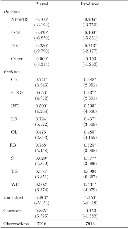
[INSERT TABLE 8: Probit Models for % Played and Produced for Overall Pool for Players]
The above figure shows the marginal effects for both the played and produced models for
30
very similar to that of expected return. The results for the division dummies are once again
similar, as the Power 5 reference group is by far the most likely to have played and produced
with non-Power 5 FBS coming in second. For the positional dummies, these models will be
interesting to present to a young prospective player, who decides that he wants to play in the
NFL but does not know which position he wants to play. In both models, quarterbacks are by far
the least likely to play and produce in the NFL, which again, as mentioned in the previous
section, reflects the overwhelming supply of quarterbacks, most of which are not very good.
Now looking specifically at the played model, wide receivers, cornerbacks, and running
backs are the most likely to play in the league above quarterbacks. These results make some
intuitive sense because in today’s NFL, the game is heavily focused on the passing game of
which wide receivers and cornerbacks are the main participants. One could argue that offensive
line should be the highest given that there are 5 offensive linemen on the field at any given time,
but a logical explanation for this is that the turnover for offensive linemen is not as high as it is
for other positions. Because wide receivers, cornerbacks, and running backs rely so much on
athleticism, as soon as there is waning athletic ability, they are more likely to be replaced and
thus have shorter careers. In addition, per Zach Binney of Football Outsiders, receivers,
cornerbacks, and running backs (and linebackers) are more likely to become injured than other
positions, which would again increase the turnover at the positions (Binney 2015). On the other
hand, offensive linemen do not have to rely as much on athleticism, so they subsist off of
technique for a longer period of time. Their injury rates are also lower compared to other
positions. Compounding these factors, there is lower turnover in personnel for offensive linemen,
31
Looking at the produced model, which again reflects whether or not a player has had a
season of significant output (here defined as having AV greater than or equal to 3), the interior
defensive linemen are the most likely to have a productive season. A possible explanation for
this is the “Planet Theory” from Bill Parcells, an esteemed football coach most famous for
coaching the New York Giants in the 1980s. He stated that there are only so many humans on the
planet that are big enough to play defensive line in the NFL. Implementing this idea between the
two models, in the played model, the percentage of interior defenders who have played are lower
relative to other positions because there are simply not enough big guys to play those spots.
However, among those who qualified to play within the NFL, they have a higher percentage of
success because the smaller interior players have already been parsed out. This theory can also
be applied to the subsequent increase that offensive linemen received between the two models.
In terms of overall efficiency of the model to correctly estimate whether or not a player
has played or produced in the NFL, the model correctly identified 92.99% and 89.72% of the
players who have played or produced respectively based on the parameters in the probit models.
Through the probit models, each player is given an estimated probability of having
played/produced in the NFL. Then they are classified as having done so if their predicted
probability is above .5, and the percent of correct predictions is calculated. With a correct
prediction percentage of 92.99% and 89.72% in the played and produced probit models, both
models work extremely well in predicting those two outcomes.
Next, for the individual position models, we will now look at the probit models solely the
quarterbacks again for consistency of analysis:
[INSERT TABLE 9: Positional Probit Played Models]
32
For the played model, the results seem closely aligned to the ones from the previous
section in terms of what characteristics NFL teams value. This would make sense as those who
share these characteristics are more likely to play. Therefore, quarterbacks with the running poor
pocket ability trait are very unlikely to play. In contrast, quarterbacks identified with having the
ability to keep their eyes downfield, which is directly opposite of the previous characteristics, are
more likely to play. An ability to read the defense is again a very likely indicator that a
quarterback would play. Negative accuracy is also not a big factor in determining the probability
that a quarterback would play or not, and quarterbacks with poor mechanics are also very
unlikely to play, specifically 42.39% less.
An interesting significant characteristic in this case is the negative spread characteristic.
In this context, this characteristic represents the fact that the quarterback came from a spread
offense, which is largely a college offense that does not have tremendous carryover to the NFL.
A reasoning behind why this characteristic could be significant is that the vast majority of
colleges now run the spread offense, so the NFL has no choice but to play these spread
quarterbacks. Whether or not a player is penalized for playing in a spread offense could be
explained by several other factors not accounted for in the study, but in this case, the players
with the negative spread characteristic are 35.62% more likely to play than those without it.
Furthermore, a couple of characteristics that do not adhere to any intuitive explanation
are the positive arm strength characteristic and the negative batted balls characteristic. One
would think that the NFL would value somebody with very good arm strength and those who
avoid getting their passes batted at the line of scrimmage. The only explanation for the
33
are not accounted for in this study. Overall, the accuracy of this model is quite proficient as it
correctly identifies 89% of the sample.
[INSERT TABLE 11: Positional Probit Played Models]
[INSERT TABLE 12: Corresponding Characteristics for Table 11]
Now looking at the produced model, the model holds similar characteristics as the played
model. This is to be expected as the produced model only indicates the fact that the quarterback
has made a notable contribution to the productivity of the offense and not the actual level of his
playing ability. Unlike other positions, there are no substitutions for quarterbacks. Thus, if a
quarterback plays a game, barring injuries or extremely poor performance, he plays the entirety
of the game. Because of the enormous impact quarterbacks have on offensive performance, a
quarterback who starts a good portion of games is likely to pass the 3 AV threshold of being a
player who “produced” in his career. The number of quarterbacks who also get to play in the
NFL is much smaller than that of other positions. Because of that, the ones who do get to play
get do so for a more prolonged period of time compared to the other positions, so the similarity
of the two models is to be expected. This same condition does not hold for other positions
because there are multiple starters for each position group, and a played designation could mean
a part-time role for other positions whereas a played designation for quarterbacks indicates a
full-time role.
To show the efficacy of the models in predicting player outcomes, a table is shown below
to show the prediction probabilities for both the overall pool of players and the individual
positions in the played and produced models.
34
The next model to analyze is the panel approximate value model for both the overall pool
of players and the position specific players. There is a stark contrast between these models and
the previous models because now the data is in panel format and is going to be analyzed with
respect to time and how the players perform over time.
[INSERT TABLE 14: Approximate Value Panel Summary]
The variation of AV in panel form follows suitable logic. Here, we deal with the AV of a
player throughout the progression of a player’s entire career. The variation of AV between
different players is greater than the variation within the same player across multiple seasons.
Players of a certain skill level are likely to play around that skill level across their career, and the
skill level between players is very different. Two different models of the overall players’ pool are
estimated here. One including the pick number of where the player was drafted and one without.
[INSERT TABLE 15: Overall Models for Panel AV Player Data]
Here the random effects model is used because most of the individual characteristics do
not vary over time, and using the fixed effects model will simply difference out the
time-invariant regressors. The most notable thing in the overall model is how experience affects
approximate value. According to the model, every year of experience significantly increases
approximate value produced by .086, which makes intuitive sense as a player is likely to become
better as they gain more experience. However, the microeconomic principle of diminishing
marginal productivity is on display as the coefficient of experience squared is negative with a
coefficient of -.0124. Combining the two coefficients, the peak returns for experience occurs
after 3 or 4 years. In other words, on average, a player reaches the peak of his value at around his
4th or 5th year or at around age 25-27, which is slightly lower than expected. This speaks to how
35
how often should teams extend their players beyond their rookie contracts. There is some
variability of the significance of experience across positions as experience is not a significant for
QBs, RBs, WRs, TEs, and CBs, but in all cases except for quarterback, the squared term is
highly significant and negative, which would imply that experience has a negative effect on
approximate value over time. Even when the squared term is removed from the regressions, the
experience term remains insignificant across the above 5 positions.
The division dummies are again similar to those of previous models with Power 5 as the
base group. In regards to the position dummies, surprisingly enough, interior defenders and wide
receivers accrue significantly more approximate value than quarterbacks. A thing to keep in
mind is that these measures are measures of individual performance and not how much they
impact the team. An extra AV for a quarterback does not have the same effect on the team as an
extra AV for a defensive tackle, but they can still be of equal skill per AV. Therefore, in this
case, the higher AV for the position dummies represents solely individual production and not
individual impact for the team.
Including pick number of where a player was drafted in the model, an interesting result
occurs. The sign for pick number is very clearly negative and significant because the lower the
pick number indicates that the player was drafted earlier. For example, a player picked 1st is
picked earlier than 14th, so the coefficient of pick number shows us that players picked earlier are
in general better than those picked later. Specifically, the coefficient of pick number is -.0436
with a z-statistic of -14.70, which means that a player picked 1 pick earlier will have .0436 more
AV. However, pick number squared is positive, which shows that there are also diminishing
marginal returns to pick number as there is for experience. The coefficient for this is .0000817
36
earlier do indeed produce more, the production gap between a player and a player picked before
him diminishes throughout the draft. The point at which the production between two players
selected 1 pick away from each other is the same is at a theoretical pick 267 (there are usually
only around 253 picks in the draft and none have come close to 267). An interesting idea to
examine in the future is examining what would be the optimal draft strategy of teams. How
should teams approach the draft where they can cost-effectively and most efficiently acquire the
most talent. The commonly held belief among many analytics-based football thinkers is that
teams should acquire as many picks as possible as they are similar to lottery picks in acquiring
productive football players, but a tweak to this approach could be to acquire as many 2nd to 4th
round picks as possible to both maximize the probability of picking a productive player and
acquiring a large number of productive players overall.
Now looking at the individual positional models, specifically quarterbacks:
[INSERT TABLE 16: Positional Panel Regressions for Approximate Value]
[INSERT TABLE 17: Corresponding Characteristics for Table 16]
There are several interesting results with this regression, but the most interesting result is
that of pick number and pick number squared. As stated before, an important consideration when
looking at the coefficients of the pick number variables is that the lower the pick number, the
more the player is valuable per the league. On average, the quarterbacks drafted earlier tend to
have higher production, and the effects of pick number squared are marginally diminishing. An
interesting but also very intuitive result is that of experience and experience squared, neither of
which are significant. Even when the experience squared term is omitted, experience remains
insignificant. There are two important interpretations of this result. First of which is that