Summer 2010
A New Approach in Fitting Linear Regression Models with the Aim of
Improving Accuracy and Power
Soheil Sadeghi1, Hashem Mahlooji2
Department of Industrial Engineering, Sharif University of Technology, Tehran, Iran
1 [email protected], 2 [email protected]
ABSTRACT
The main contribution of this work lies in challenging the common practice of inferential statistics in the realm of simple linear regression for attaining a higher degree of accuracy when multiple observations are available, at least, at one level of the regressor variable. We derive sufficient conditions under which one can improve the accuracy of the interval estimations at quite affordable extra computational cost. Two algorithms and a numerical example will be presented to fully explain how our approach works and to compare the results of our approach versus the results obtained from three of the well known statistical software systems.
Keywords: Simple linear regression, Multiple observations, Weighted least squares, Accuracy,
Power 1. INTRODUCTION
Linear regression models are among the most popular statistical tools which have been successfully applied to a wide spectrum of problems. To apply regression models, the common practice is to collect data and minimize the sum of squared deviations between the observed data and the values coming from the underling relation, Montgomery et al. (2001) and Neter et al. (1996). Once the regression model is developed, various tests of hypothesis as well as confidence and prediction intervals can be presented.
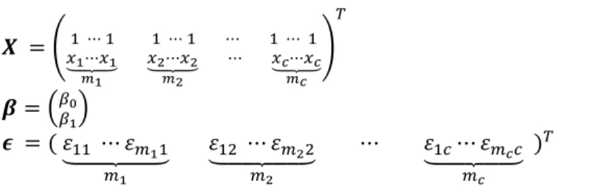
Here, we start with the simple linear regression model shown in (1) which we label as the
throughout the article:
. (1)
where
⋯ ⋯ … ⋯
Corresponding Author
⋯ ⋯ ⋯ ⋯ ⋯ ⋯ ⋯ ⋯
⋯ ⋯ ⋯ ⋯
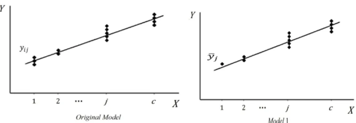
In this model there are , 1,2,3, … , observations from the response variable, , at each of
the levels of the regressor variable, , such that there are pairs of data altogether (see Figure 1). For the sake of our discussion it suffices for just one to be strictly larger than 1.
This means that , ∑
Figure 1 The layout of data in the
The commonly adopted assumptions in regression analysis include:
0 ; 1, 2, … , (2)
; 1, 2, … , (3)
, 0 ; , 1, 2, … , (4)
Assuming that ’s behave as normal random variables, appropriate confidence and prediction intervals can be presented. Since it is possible that the unknown variances in (3) not to be fixed for all ′s, one can adopt the weighted least squares to treat such a case.
The commonly adopted approach toward statistical inference in the regression problem as outlined above, often fails to exploit all the potential that the collected data has to offer in order to arrive at
the best possible results. In this work we analytically establish the conditions under which such
potential is practically wasted while by bearing a very affordable cost one could have achieved more accurate results. In the quest for identifying the optimal (regression) model, i.e., the model that better exploits the potential of the collected data, we present two algorithms and by borrowing a typical problem from literature we extensively demonstrate how our proposed approach works and what it can achieve when compared with the approach which is commonly practiced.
This paper is organized in the following manner: section 2 investigates a model in which the mean of observations at just one level of the independent variable takes the place of the observations
themselves. We examine to see if relations (2), (3), and (4) are still true for such a case and then arrive at the regression model. Section 3 presents a similar discussion when the means of observations at more than one level of the independent variable are considered. Section 4 presents
an algorithm for finding a model with the smallest mean squared error ( ). Section 5 is devoted
to generating a model with the largest accuracy. Section 6 includes a numerical example. Section 7 concludes the discussion and presents some ideas for further investigation.
2. REGRESSION ON THE MEAN OF OBSERVATIONS AT A SINGLE LEVEL
In this section we assume that at a single level of the regressor variable we have available
1 , 1,2, … , observations on . Since it is irrelevant at which level of these multiple
observations are collected, here we assume that the observations correspond to the level
where 1 and we intend to employ the mean of these observations in fitting the regression
model. As such, we are dealing with the following model which we label as where 1
(unless specified otherwise).
. (5)
in which
∑ ⋯ ⋯ ⋯
is an 1 1 matrix,
⋯ ⋯ ⋯ ⋯ ⋯ ⋯
is an 1 2 matrix,
,
and finally,
∑ ⋯ ⋯ ⋯
is an 1 1 matrix.
To arrive at the regression model in (5) we first present the following definitions:
:represents an 1 matrix of the form
1 … 1 0 0 … 0
0 … 0
0 … 0
⋮ ⋱ ⋮
0 … 0
1 0 … 0
0 1 … 0
⋮ ⋮ ⋱ ⋮
where in the first row the first entries are 1 and the remaining entries are 0. In the lower right
side of there is an unit sub-matrix and all other entries of are 0.
:stands for an 1 1 matrix of the form
0 … 0
0 ⋮ 0
1 ⋮ 0
… ⋱ …
0 ⋮ 1
where each of its off diagonal entries is zero, and all diagonal entries are except for the entry at northwest corner which is 1/m1.
We have defined and in a way such that by multiplying both sides of (1) by . one can
arrive at 1.
2.1. Parameter Estimation
We first examine to see if (2), (3), and (4) hold in 1. As can be seen below, (2) and (4) hold
true while this is not the case for (3). To get around this problem we resort to weighted least squares to fit our model.
∑ 0 ∑
0 ; 2, … , 1
∑
; 2, … , 1
, ∑ , 0 ; 2, … , 1
, 0 ; , 2, … , 1
Therefore
0 0 ⋯ 0 and
0 … 0
0 ⋮ 0
1 ⋮ 0
… ⋱ …
0 ⋮ 1
It is clear that the weighted least squares (WLS) estimators of the parameters in 1 can be
written as Neter et al. (1996).
. . . . . (6)
Now, we establish the fact that is exactly the sameas . . . which represents
the least squares (LS) estimators of the . To show this we substitute and in
(6) by . . and . . respectively to obtain
. . . . . . .
noting that and . , we will have . . . . . .
1 ⋮ 1
0 … 0
⋮ ⋱ ⋮
0 … 0
0 ⋮ 0
1 … 0
⋮ ⋱ ⋮
0 … 1
.
0 … 0
0 ⋮ 0 1 ⋮ 0 … ⋱ … 0 ⋮ 1 .
1 … 1 0 0 … 0
0 … 0
0 … 0
⋮ ⋱ ⋮
0 … 0
1 0 … 0
0 1 … 0
⋮ ⋮ ⋱ ⋮
0 0 … 1
1 ⋮ 1
0 … 0
⋮ ⋱ ⋮
0 … 0
0 ⋮ 0
1 … 0
⋮ ⋱ ⋮
0 … 1
.
⋯ 0 0 … 0
0 … 0
0 … 0
⋮ ⋱ ⋮
0 … 0
1 0 … 0
0 1 … 0
⋮ ⋮ ⋱ ⋮
0 0 … 1
1⁄ … 1⁄
⋮ ⋱ ⋮
1⁄ … 1⁄
0 … 0
⋮ ⋱ ⋮
0 … 0
0 … 0 ⋮ ⋱ ⋮ 0 … 0
1 … 0
⋮ ⋱ ⋮
0 … 1
Designating this matrix by , we have
. ⋯ ⋯ ⋯ ⋯ ⋯ ⋯ ⋯ ⋯ .
1⁄ … 1⁄
⋮ ⋱ ⋮
1⁄ … 1⁄
0 … 0
⋮ ⋱ ⋮
0 … 0
0 … 0 ⋮ ⋱ ⋮ 0 … 0
1 … 0
⋮ ⋱ ⋮
0 … 1
therefore, having in mind that . . and . , one can write
. . . . . . . . . . . . . .
. . .
As can be seen, the LS estimators for 5 are exactly the same as those obtained for the
. The variance of the coefficients in the is
.
and since in 1 is the same as (in the ), then obviously
.
2.2. The Sum of Squares
2.2.1. The Sum of Squared Error ( )
So far we have shown that the estimated regression line in 1 coincides with the one in the
Figure 2 Data layout for the and 1 around the line of regression
It is evident that the sum of squared errors ( ) differ for the two models only at level . In fact,
’s for the two models have identical terms at all the other levels of the regressor variable. Let
and designate the sum of squared errors in the O and the proposed model
( 1) respectively. Thus we can write
∑ ∑ ∑ ∑ ∑
. ∑ ∑
Where stands for the expected value of the dependent variable at level of the regressor variable.
To set up a relation between and , we can write
∑
∑ 2 2
∑ ∑
this means that , where ∑ .
In other words, when the mean of observations is used instead of the observations
themselves, will be reduced by as much as ∑ .
2.2.2. The Total Sum of Squares ( )
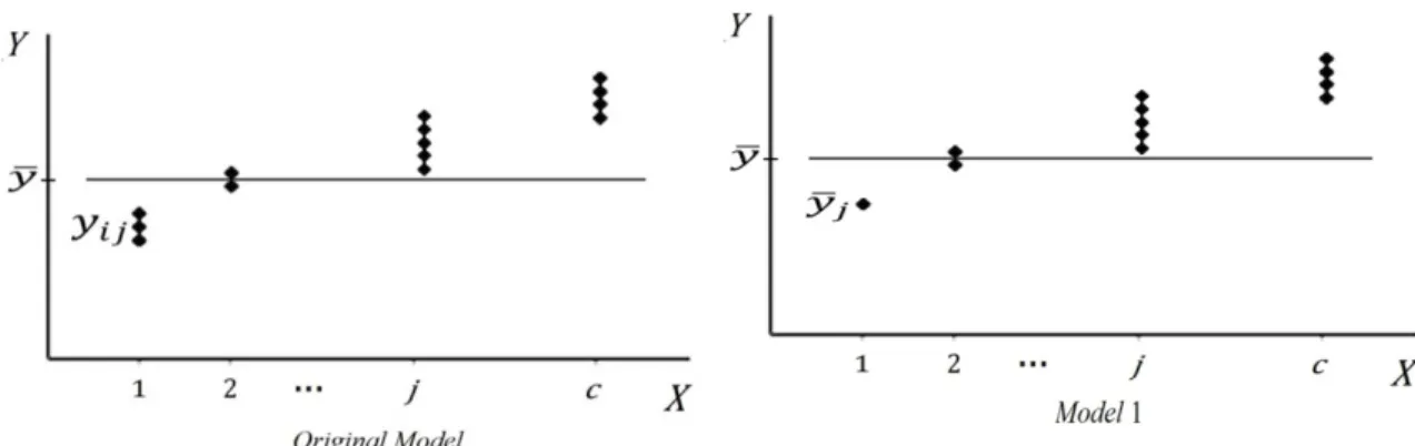
To compare for the and 5 we first calculate the mean of the observed
values of the response variable for 5 as
∑ ∑ ∑ ∑
Figure 3 Layout of data around for the and 1
As expected, the mean of the observed values of in both models are identical. Now, according to the situations displayed in Figure 3, for the , , and the proposed model, , can be written as
∑ ∑ ∑ ∑ ∑
. ∑ ∑ .
These differ by as much as
∑
∑ 2 2
∑ ∑
which means that
,
where ∑ , as before.
The last equation above reveals that by regressing on the mean of the observed values of at level ,
tends to decrease as much as .
2.2.3. The Sum of Squares due to Regression ( )
Since holds so does the relation , which means that is the
same for both models.
2.3. The Mean Squared Error ( )
To compare the ’s of the and 1, i.e., and , we can write
2 1
or finally
2
This means that for the proposed model to reduce the , it is sufficient to have
2
or
. . Or, finally, we have
(7) where
∑ .
It is interesting to note that both and are unbiased estimators of and in case the
relation (7) holds, the in the proposed model will be smaller than that in the .
Besides, as shown earlier, the variances of the coefficients in both models are identical and equal to
.
Employing the unbiased estimators of here, leads to the following point estimators for variances
of the coefficients:
. : .
1: .
It is clear that forcing ensures us that the estimators of variance of the coefficients in
the proposed model tend to decrease in comparison to the corresponding estimates from the
.
2.4. Coefficient of Determination
As far as the coefficient of determination is concerned, one can write
and
for the original and the proposed models. Now, the following relation shows that employing the
2.5. Power of the Tests and the Length of the Intervals
To judge the power of the tests as well as the length of the confidence and prediction intervals, in this section we assume that the error terms behave as normal random variables.
2.5.1. Judging the Parameter Estimators
The two-sided 100 1 % confidence interval for parameter , 1,2 for the proposed
model can be written as
; . , 0,1
where is the square root of the estimated variance of the point estimator of .
The length of this interval reflects upon the interval’s accuracy and the power of the corresponding test in the sense that the shorter this interval, the higher the accuracy as well as the power would be. Employing the proposed model will decrease the degrees of freedom and in spite of the fact that
, the value of and consequently the values of tend to decrease. As such, for
comparing the accuracy and the power in employing the two models it would be sufficient to compare the term
; . . . √ (8)
in the two models. Whenever this term for one of the models is smaller, that model provides a higher degree of accuracy and more power.
2.5.2. Inferring on the Mean of the Response Variable at a Fixed Level of the Independent Variable
A two-sided 100 1 % confidence interval for the expected value of the response variable at
the level assumes the following form
; . (9)
where represents the value that the estimated line assumes when and is defined
as
. . . .
in which .
A comparison of confidence intervals presented in (9) for the two regression models leads again to the comparison of (8) for these models.
2.5.3. Inferring on a New Observation of the Response Variable at a Specified Level of
The prediction interval for a new observation of the response variable when is considered at level can be written as
; .
where
. 1 . . .
Once again, comparing this interval for the two models leads to a comparison of (8) for them.
Our findings so far indicate that decreasing by itself is not a sufficient yardstick for attaining
more accuracy and power and we showed instead that we should see to it that the following holds true:
; . ; .
or
;
;
2
or
;
;
2 1
or
2 ;
;
or
2 1 ;
;
or
2 1 ;
;
,
and, finally, we have
1 ;
;
This means that once (10) holds, the proposed approach generates more powerful tests and more accurate confidence and prediction intervals.
3. EMPLOYING OBSERVATIONS’ MEANS AT MORE THAN ONE LEVEL
3.1. Means at Two Levels
Let and represent the levels at which multiple measurements from the response variable are
available. We intend to employ means of such observations in fitting the regression model. To
achieve this purpose one can develop the intended model based on either the or
5. In fact, the model will look like the following which we label as , ,
1, 2 meaning the model in which means are employed at levels and of the regressor variable.
, , . , (11)
in which , and , represent 2 1 matrices, i.e.,
, ⋯ ⋯ ⋯
and
, ̅ ̅ ⋯ ⋯ ⋯
and , represents the following 2 2 matrix
, ⋯ ⋯ ⋯ ⋯ ⋯ ⋯
Here, , , ̅ , and ̅ represent the means of the observed data as well as the means of error terms
at levels and respectively.
To arrive at the model in (11), it suffices to multiply both sides of (5) by the matrix combination
1 0
0 ⁄
0 … 0
0 … 0
0 0 ⋮ ⋮ 0 0
1 … 0
⋮ ⋱ ⋮
0 … 1
.
1 0 … 0
0 1 … 1
0 … 0
0 … 0
0 0 … 0
⋮ ⋮ ⋱ ⋮
0 0 … 0
1 … 0
⋮ ⋱ ⋮
0 … 1
where and are 2 2 and 2
1 matrices. It is quite straightforward to show that relations (2) and (4) hold for the
model in (11). One can resort to the weighted least squares to get around the nonhomogeneity of variances of the errors.
,
⁄ 0 0 ⁄
0 … 0
0 … 0
0 0 ⋮ ⋮ 0 0
1 … 0
⋮ ⋱ ⋮
0 … 1
the weighted least squares point estimators of the coefficients can be obtained. Specifically, in
suffices for , to take the place of in (6) and and be substituted by , and ,
respectively. Here, again it will be a simple matter to show that the point estimators are exactly the
same as the estimators in 1 and hence, in the .
Similar to what was shown, again it can be shown that ,
and
, ,
and
, .
As before, when ∑ holds, employing the model in (11) tends
to decrease the when compared to 1. Now we derive the conditions under which the
model in (11) provides a smaller compared to the .
In order for the inequality , to be true, we should have
or
,
where ∑ , 1,2.
This point must be stressed that if 1 1 achieves a lower than the
, and hence if 2 2 achieves an smaller than that of the
, it would be reasonable to conclude that 1,2 1, 2 will follow
suit. The opposite of this argument is not necessarily true. In fact, it is possible for either of
1 or 2 to have an higher than that of the while 1,2
achieves a lower than the . Under these circumstances, it can be asserted that
either of 1 or 2 will certainly lower the as that achieved by the
. This point can be explained in mathematical terms as follows.
If ⇒ 1 , and
⇒ 1 , then
The next important point is that if both 1 and 2 achieve lower than the provided
by the , it can be concluded that 1,2 achieves an lower than what
provided by both 1 and 2. This is because: if ⇒ and
since , then . Therefore we obtain
, .
In like manner, if ⇒ , and since then
. Therefore we obtain
, .
We conclude this section by pointing to the fact that 1,2 can be directly obtained from the
. To show this fact, one can simply multiply both sides of (1) by the following
2 2 and 2 matrix combination
⁄ 0 0 ⁄
0 … 0
0 … 0
0 0 ⋮ ⋮ 0 0
1 … 0
⋮ ⋱ ⋮
0 … 1
.
1 … 1 0 … 0
0 … 0 1 … 1
0 … 0
0 … 0
0 … 0 0 … 0
⋮ ⋱ ⋮ ⋮ ⋱ ⋮
0 … 0 0 … 0
1 … 0
⋮ ⋱ ⋮
0 … 1
3.2. Employing the Mean Observation Values at All Levels of the Independent Variable
Here we assume that the number of observations of the response variable at each level of the
independent variable is strictly larger than 1. As such, our model labeled as 1,2, … , will
look like
, ,…, , ,…, . , ,…, (12)
Where
, ,…, ⋯ , ,…, ⋯ ⋯
, ,…, ̅ ̅ ̅ ⋯ ̅
in which , ,…, and , ,…, are 1 matrices and , ,…, is a 2 matrix. One can arrive at this
⁄ 0
0 ⁄
0 … 0 0 … 0 0 0
⋮ ⋮ 0 0
⁄ … 0 ⋮ ⋱ ⋮ 0 … ⁄
.
1 … 1 0 … 0
0 … 0 1 … 1
… 0 … 0
… 0 … 0
⋮ ⋱ ⋮ ⋮ ⋱ ⋮
0 … 0 0 … 0
⋱ ⋮ ⋱ ⋮
… 1 … 1
Again, it can be simply shown that (2) and (4) hold. Also, we employ that weighted least squares to resolve the lack of homogeneity of the variances of the error terms. The following shows that the fitted model is the same as the original fitted model.
, ,…, ∑
, ,…, ∑
, ,…,
The relations that immediately follow, intend to establish this fine point that in
1,2, … , is the lowest value among all possible models’ ’s and is equal to the lack of fit
sum of squares ( ) in the . In other words, while in the
assumes its largest value, it assumes its smallest value in 1,2, … , . We know that
,
or
∑ ∑ ∑ . (13)
then
, ,…, .
Therefore, we can write
, ,…,
, ,…,
All this means that assumes its largest value in 1,2, … , and its smallest value in the
. This assertion follows from the fact that , , ,…, , ,…,
, ,…, and (13)
is true.
4. IDENTIFYING THE MODEL WITH THE SMALLEST
In this section we explain how one can easily identify the model with smallest from among
the existing models. Assuming 2 at levels , then there are as many as 2 models
including the . The following algorithm is proposed to find the model with
smallest .
Algorithm 1
Step 2: Compute and check the condition , ∀ .
If this inequality is not true for any, or if there is no remaining to be considered, stop and treat
as the smallest and the corresponding model is the model with smallest .
Otherwise go to Step 3.
Step 3: Consider the level(s) at which the inequality in Step 2 is satisfied; employ the mean of
observations instead of the observations at each level and set equal to the obtained
from this model; return to Step 2 for examining the remaining levels.
The discussion presented in section 3.1 provides the motivation for explaining why this algorithm is
expected to identify the model with smallest .
It is obvious that by itself is not a suitable criterion in comparing the existing models because
the model which lowers the faces a decrease in the degrees of freedom as well. In fact, one
should judge based on relation (8) in the sense that the model with smallest value of (8) will be the best linear fit on the basis of the power of the tests as well as the accuracy of the prediction and confidence intervals.
5. IDENTIFYING THE MODEL WITH THE LARGEST ACCURACY
Assuming that at out of levels of the independent variable, 2 holds, we intend to identify
the best model on the basis of power of the tests. We try to minimize
; . . . √
Based on a table of t-distribution, one can prepare a table for tabulating different values of
; . . . . . ; . .
for various values of and degrees of freedom. Thus this problem assumes the following form
; . . . ∑ .
where ′ are decision variables assuming value 0 or 1.
. . ∑ ∑ 2 .
One way to identify the most powerful and the most accurate model would be comparing the objective function for all possible cases and determining the smallest value of (8) for the existing models.
5.1. The Case of Identical Number of Multiple Observations at Selected Levels of the Independent Variable
Suppose we are dealing with a problem in which there are an identical number of multiple
special case of the problem as presented in section 3.1. The difference lies in the fact that for this problem one can come up with a simple algorithm to identify the optimal model based on the power of the tests and the accuracy of the confidence intervals.
The interesting point is that based on the nature of the reduction in the degrees of freedom one can
easily identify the optimal model. The reduction of degrees of freedom in ,
1,2, … , amounts to 1. There are as many as of such models. This number for
, stands at 1 and the reduction in the degrees of freedom is as much as
2 1 . In general, when there are levels of the independent variable, the reduction of the
degrees of freedom amounts to 1 and there will be of such cases. In models with
identical degrees of freedom, the term
; . . in ; . . . √ remains the same and it
suffices to concentrate on which consists of two parts: and a quantity which must be
subtracted from .
Since is the same for all models, then among the models with the same degrees of freedom the
model in which the largest quantity is subtracted from corresponds to the objective function
with the smallest value. Thus we propose the following algorithm to identify the optimal model.
Algorithm 2
Step 1: compute at each level and sort them in descending order as
⋯ .
Step 2: compare the objective function for the following 1 models and deliver the optimal model.
, 1
, 1 , 2
⋮
, 1 , … , 2
, 1 , … , 2 , 1
where, for example, , 1 represents the model at levels and 1 such that
the level with the largest value of and 1 the level with the second largest value of
.
It must be noted that this algorithm needs just 1 and not 2 comparisons to deliver the optimal
model.
6. NUMERICAL EVALUATIONS
In this section we provide a detailed example to shed light on the merits of our approach. To this end we borrow the following example from Neter et al. (1996).
Example (Problem 20, page 38): Calculator maintenance. The Tri-City Office Equipment
Corporation sells an imported desk calculator on a franchise basis and performs preventive maintenance and repair service on this calculator. The data below have been collected from 18 recent calls on users to perform routine preventive maintenance service; for each call, x is the number of machines serviced and y is the total number of minutes spent by the service person.
Assume that first-order regression model ( ) is appropriate.
: 1 2 3 4 5 6 7 8 9 10 11 12 13 14 15 16 17 18
: 7 6 5 1 5 4 7 3 4 2 8 5 2 5 7 1 4 5
: 98 86 78 10 75 62 101 39 53 33 118 65 25 71 105 17 49 68
As Table 1 shows, there are 18 pairs of observations in this problem gathered at 8 levels of the regressor variable. At 5 levels of we have more than one observation on the dependent variable.
Table 1 values of for 1, … ,8
1 10 , 17 13.500 24.500 24.500
2 33 , 25 29.000 32.000 32.000
3 39
4 62 , 53 , 49 54.667 88.667 44.333
5 78 , 75 , 65 , 71 , 68 71.400 109.200 27.300
6 86
7 101 , 98 , 105 101.333 24.667 12.333
8 118
By feeding these data to SAS (Statistical Analysis System) we arrive at the following model
2.322 14.738
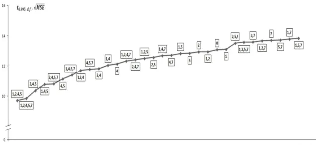
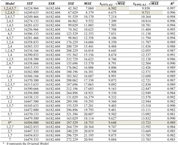
Table 2 displays the outcome of all calculations for all possible cases. Figures 4 and 5 display the same results graphically.
The most common values of 1% and 5% for are used in Table 2, Figure 4, and Figure 5.
Table 2 Summary of calculations for 32 models
Model . ; . .. √ . ; . . . √
1,2,4,5,7 16224.966 16182.604 42.362 7.060 6.502 9.850 0.997
1,2,4,5 16249.633 16182.604 67.029 8.379 6.675 9.711 0.996
2,4,5,7 16249.466 16182.604 91.529 10.170 7.214 10.364 0.994
2,4,5 16274.133 16182.604 66.862 9.552 7.309 10.814 0.996
1,4,5 16281.633 16182.604 99.029 11.003 7.503 10.781 0.994
1,4,5,7 16256.966 16182.604 74.362 10.623 7.708 11.404 0.995
4,5 16306.133 16182.604 123.529 12.353 7.831 11.138 0.992
4,5,7 16281.466 16182.604 98.862 12.358 8.106 11.794 0.994
1,2,4 16358.833 16182.604 176.229 14.686 8.350 11.707 0.989
2,4 16383.333 16182.604 200.729 15.441 8.488 11.836 0.988
1,2,4,7 16334.166 16182.604 208.229 16.018 8.645 12.055 0.987
1,4 16390.833 16182.604 151.562 15.156 8.674 12.337 0.991
1,2,5 16338.300 16182.604 232.729 16.623 8.746 12.138 0.986
2,4,7 16358.666 16182.604 155.696 15.570 8.791 12.504 0.990
4 16415.333 16182.604 176.062 16.006 8.806 12.426 0.989
2,5 16362.800 16182.604 180.196 16.381 8.908 12.571 0.989
1,4,7 16366.166 16182.604 183.562 16.687 8.991 12.688 0.989
1,5 16370.300 16182.604 208.062 17.338 9.073 12.721 0.987
1,2,5,7 16313.633 16182.604 187.696 17.063 9.092 12.830 0.989
4,7 16390.666 16182.604 212.196 17.683 9.163 12.847 0.987
5 16394.800 16182.604 264.896 18.921 9.330 12.949 0.984
2,5,7 16338.133 16182.604 131.029 16.379 9.332 13.578 0.992
1,2 16447.500 16182.604 289.396 19.293 9.360 12.944 0.982
1,5,7 16345.633 16182.604 155.529 17.281 9.403 13.510 0.990
2 16472.000 16182.604 296.896 19.793 9.481 13.111 0.982
5,7 16370.133 16182.604 321.396 20.087 9.502 13.092 0.981
1 16479.500 16182.604 163.029 18.114 9.627 13.832 0.990
0* 16504.000 16182.604 187.529 18.753 9.648 13.723 0.989
1,2,7 16422.833 16182.604 264.729 20.364 9.747 13.592 0.984
2,7 16447.333 16182.604 240.229 20.019 9.749 13.669 0.985
1,7 16454.833 16182.604 296.729 21.195 9.875 13.705 0.982
7 16479.333 16182.604 272.229 20.941 9.884 13.783 0.983
* 0 represents the
As can be seen, for 0.01 and 0.05 1,2,4,5 and 1,2,4,5,7 are the best models respectively. Also, the ratio of the lengths confidence and prediction intervals of the
proposed best models to those of the which is commonly used in practice are
α 0.05 ∶ t . ; . . . √MSE 6.502 ; Model 1,2,4,5,79.648 ; Original Model → .
. 0.673
α 0.01 ∶ t . ; . . . √MSE 13.723 ; Original Model9.711 ; Model 1,2,4,5 → .
. 0.708
All this means that 1,2,4,5 and 1,2,4,5,7 are capable of reducing the lengths of the
confidence and prediction intervals by %29.2 and %32.7 for 0.01 and 0.05 respectively
when compared to the without any cost.
7. CONCLUSIONS
In this work we showed how one can improve the accuracy of the confidence and prediction intervals in simple linear regression at no cost.
Our treatment has been confined to the problems with multiple observations on the dependent variable at some levels of the regressor variable. In fact, by presenting an algorithm we showed that
it suffices to identify the model with smallest value of ; . . . √ at a given level of , to
arrive at more accurate confidence and prediction intervals.
Extensions to this work consist of designing a more sophisticated algorithm to identify the model
with the smallest ; . . . √ ; designing statistical tests and test statistics for comparing
different models; and investigating the multiple regression models. Developing a computer code in R system to implement this approach is another avenue for future research.
REFERENCES
[1] Montgomery D.C., Peck E.A., Vining G.G. (2001), Introduction to Linear Regression Analysis; 3rd
edition, Wiley.
[2] Neter J., Kutner M.H., Nachtsheim C.J., Wasserman W. (1996), Applied Linear Regression Models; 3rd edition, Irwin.
[3] MINITAB® Release 14.12.0, http://www.minitab.com, September 2010. [4] R 2.11.1 system, http://www.r-project.org, September 2010.