Sharif University of Technology
Scientia IranicaTransactions D: Computer Science & Engineering and Electrical Engineering http://scientiairanica.sharif.edu
Solution to fractional-order Riccati dierential
equations using Euler wavelet method
A.T. Dincel
Department of Mathematical Engineering, Davutpasa Campus, Yildiz Technical University, 34220, Esenler, Istanbul, Turkey. Received 24 June 2018; received in revised form 27 September 2018; accepted 3 October 2018
KEYWORDS Euler wavelet; Fractional calculus; Operational matrix; Numerical solution; Riccati dierential equations.
Abstract.The Fractional-order Dierential Equations (FDEs) have the ability to model the real-life phenomena better in a variety of applied mathematics, engineering disciplines including diusive transport, electrical networks, electromagnetic theory, probability, and so forth. In most cases, there are no analytical solutions; therefore, a variety of numerical methods have been developed for obtaining solutions to the FDEs. In this paper, we derive numerical solutions to various fractional-order Riccati-type dierential equations using the Euler Wavelet Method (EWM). The Euler wavelet operational matrix method converts the fractional dierential equations to a system of algebraic equations. Illustrative examples are included to demonstrate validity and eciency of the technique.
© 2019 Sharif University of Technology. All rights reserved.
1. Introduction
Fractional Dierential Equations (FDEs) have dier-entiator operators of non-integer orders. There has been an increasing interest in modeling using FDEs, since they have the ability to model the real-world phenomena more accurately in a variety of disciplines such as visco-elasticity [1], solid mechanics [2], bioengi-neering [3,4], economics [5], continuum mechanics [6], signal processing [7], system analysis [8], optimal control [9,10], and numerical solutions to integral and dierential equations [11-13]. Since most of the fractional-order dierential equations do not have ana-lytical solutions, there have been numerous numerical methods developed to attain solutions to them, includ-ing Adomian Decomposition Method (ADM) [14,15], Variational Iteration Method (VIM) [16], Fourier trans-forms [17], Laplace transtrans-forms [18], eigenvector
expan-*. Tel.: +90 212 3834610
E-mail address: [email protected] doi: 10.24200/sci.2018.51246.2084
sion [19], Homotopy Perturbation Transform Method (HPTM) [20,21], and various wavelet methods [22-25]. In many areas of engineering and applied sci-ence, such as transmission-line phenomena, optimal ltering, network synthesis, robust stabilization, image processing, control theory, etc., Riccati dierential equations are utilized. Recently, various numerical methods [26-29] have been developed to solve Riccati dierential equations. As for the numerical methods for fractional Riccati dierential equations, Yuzbasi [30] developed a numerical method using the Bernstein polynomial; Mabood et al. [31] used the Optimal Homotopy Asymptotic Method (OHAM); Li et al. [32] applied a Reproducing Kernel Method (RKM); Odi-bat and Momani [33] used the Modied Homotopy Perturbation Method (MHPM); Khader [34] used the fractional Chebyshev nite dierence method; and Sakar et al. [35] applied an Iterative Reproducing Kernel Hilbert Space Method (IRKHSM) to get the solutions to fractional Riccati dierential equations.
In this paper, we consider the following Riccati dierential equations of the form:
t > 0; n < n + 1; (1) which is subject to the initial conditions yk(0) = g
kand
k = 1; 2; ; n 1, where is the fractional derivative-order parameter; n is an integer; u(t), v(t), and w(t) are given functions; and gk is a constant.
When is a positive integer, the fractional equa-tion becomes a classical Riccati dierential equaequa-tion.
The wavelet theory is one of the popular areas in applied science and engineering, such as segmenta-tion, data compression, and time-frequency analysis. Wavelets generally provide accurate modeling in both time and frequency domains. Moreover, it is possible to develop fast numerical algorithms using wavelets [36]. The main advantage of using wavelet methods is that, after the discretization process, the obtained coecient matrix of the algebraic equations is a sparse matrix, which decreases the computational load and expedites the simulation.
The focus of this paper is on solving the fractional Riccati dierential equations by using Euler wavelets. The Euler wavelets are constructed by Euler polyno-mials. The method consists in reducing the fractional dierential equation to a system of algebraic equations with unknown coecients by using Euler wavelets. Even though the Euler polynomials are not based on orthogonal functions, they have the operational matrix of integration. In addition, numerical examples have demonstrated that the Euler wavelet performs better in approximating an arbitrary function than the Legendre and the Chebyshev wavelets do [37].
The structure of the paper is as follows: In Section 2, we present some basic denitions and properties of the fractional calculus. In Section 3, the Euler wavelets are constructed and the Euler Wavelets Operational Matrix of the Fractional In-tegration (EWOMFI) is derived. In Section 4, we apply EWM to the solution to the fractional Riccati dierential equations through numerical examples; and the conclusion is presented in Section 5.
2. Preliminary concepts
In this section, we present denitions for the prelimi-nary fractional calculus used in the paper.
Denition 1. The Riemann-Liouville fractional in-tegral operator of order is given as:
(If)(t) =
8 > < > :
1 ()
t
R
0 f()
(t )1 d > 0; t > 0;
f(t) = 0
9 > = > ;(2): For 0, 0, a 0, and 1, we have the following properties of the Riemann-Liouville fractional
integral:
i) II= II; (3)
ii) I(If(t)) = I(If(t)) = I+f(t); (4)
iii) I(t a)= ( + 1)
( + + 1)(t a)+: (5)
The Riemann-Liouville fractional derivative is dened by:
(Df)(t) =d
dt
n
(In f)(t);
0 n 1 < n; (6)
where n is an integer and t > 0. However, the derivative of the Riemann-Liouville operator has cer-tain shortcomings in modeling real-world phenomena. Therefore, in this paper, we use the modied version of the fractional dierential operator D proposed by
Caputo, which is given in the following denition. Denition 2. The Caputo denition of the fractional derivative operator is given by the following expression:
(Df)(t)
= 8 > > > < > > > :
dnf(t)
dtn = n 2 R
1 (n )
t
R
0
f(n)()
(t )1 n+d 0n 1<n
9 > > > = > > > ; :
(7) The relation between Riemann-Liouville operator and Caputo operator can be expressed by the following two common equations:
(DIf)(t) = f(t); (8)
and:
(IDf)(t) = f(t) n 1X k=0
f(k)(0+)tk
k!: (9)
The reader is referred to [18] for more details about fractional dierentiation and integration.
3. Derivation of the operational matrix of fractional integration for Euler wavelets 3.1. Wavelets and Euler wavelets
Wavelet analysis uses localized wavelike functions called `wavelets.' A family of wavelets consists of a mother wavelet and dilated and translated versions of the mother wavelet. By making the dilation parameter a and the translation parameter b vary continuously, we
can obtain the following family of continuous wavelets as [24]:
a;b(t) = jaj 1=2
t b
a
; a; b 2 R; a 6= 0:
(10) If the translation and dilation parameters are chosen to have discrete values, a = a0k, b = nb0a0k, a0 > 1,
b0> 0, where n and k are positive integers, the family
of discrete wavelets is obtained as:
kn(t) = ja0jk=2 (ak0t nb0): (11)
Euler wavelets nm = (k; ~n; m; t) have 4 arguments:
~n = n 1, n = 1; 2; 3; ; 2k 1; k can take any positive
integer value; m is the order for Euler polynomials; and t is the normalized time. Euler wavelets dened on the interval [0, 1) yield:
nm(t)
= (
2k 12 E~m(2k 1t n+1); n 1
2k 1t<2k 1n
0; otherwise ) ; (12) and: ~ Em(t) =
8 > > > < > > > :
1; m = 0
1 r
2( 1)m 1(m!)2
(2m)! E2m+1(0)
; m > 0 9 > > > = > > > ; ; (13)
where m = 0; 1; 2; ; M 1 and n = 1; 2; 3; ; 2k 1.
The coecient r 1
2( 1)m 1(m!)2
(2m)! E2m+1(0)
is for normality, the dilation parameter is a = 2 (k 1), and the
trans-lation parameter is b = ~n2 (k 1). E
m(t) represents
the Euler polynomials of the order m and given as follows [38]: m X k=0 m k
Ek(t) + Em(t) = 2tm; (14)
where
m k
is the binomial coecient. The rst few Euler polynomials yield:
E0(t) = 1; E1(t) = t 12; E2(t) = t2 t;
E3(t) = t3 23t2+14; : (15)
3.2. Function approximation
A function f(t) dened over [0,1) may be expanded by
Euler wavelets as: f(t) =
2Xk 1
n=1 M 1X m=0
cnm nm(t) = CT (t); (16)
where superscript T indicates transposition, and C and (t) are 2k 1 1 vectors given as:
C = [c10; c11; ; c1(M 1); c20; c21; ; c2(M 1);
; ; c2k 10; c2k 11; ; c2k 1(M 1)]T;
(17) = [ 10; 11; ; 1(M 1); 20; 21; ; 2(M 1);
; ; 2k 10; 2k 11; ; 2k 1(M 1)]T:
(18)
Now, let us dene m0 = 2k 1M. The Euler wavelet
matrix is dened as:
m0m0 = (t1); (t2); (t3); ; (tm0); (19)
where ti represents collocation points. If the
colloca-tion points are chosen as ti=i 0:5m0 , i = 1; 2; 3; ; m0,
the Euler wavelet matrix for k = 2, M = 3, and = 0:5 becomes:
m0m0(t) =
2 6 6 6 6 6 6 4
1:4142 1:4142 1:4142
0:2357 0 0:2357
0:0802 0:1443 0:0802
0 0 0
0 0 0
0 0 0
0 0 0
0 0 0
0 0 0
1:4142 1:4142 1:4142
0:2357 0 0:2357
0:0802 0:1443 0:0802
3 7 7 7 7 7 7 5 : (20)
3.3. Euler wavelet operational matrix of fractional integration
3.3.1. Block pulse functions
An m0 set of Block Pulse Functions (BPFs) is dened
as: bi(t) =
(
1 (i 1)=m0 t < i=m0
0 otherwise
)
; (21)
where i = 1; 2; 3; ; m0. The function b
i(t) is disjoint
and orthogonal. For t 2 [0; 1): bi(t)bj(t) =
(
0 i 6= j
bi(t) i = j
)
; (22)
1
Z
0
bi()bj()d =
(
0 i 6= j
1=m0 i = j
)
: (23)
dened in [0,1) can be expanded into an m0set of BPFs
as:
f(t) = m
0
X
i=1
fibi(t) = fTBm0(t); (24)
where:
f = [f1; f2; ; fm0]T;
Bm0(t) = [b1(t); b2(t); ; bm0(t)]T;
and fi is given as:
fi= m10 i=mZ 0
(i 1)=m0
f(t)bi(t)dt: (25)
The Euler wavelet matrix can also be expanded to an m0 set of BPFs as:
(t) = m0m0Bm0(t): (26)
The block pulse operational matrix for fractional inte-gration F is dened as [39]:
(IB
m0) (t) FBm0(t); (27)
where:
F= 1
m
1 (+2)
2 6 6 6 6 6 6 6 4
1 1 2 3 m0 1
0 1 1 2 m0 2
0 0 1 1 m0 3
... ... ... ... ... ...
0 0 0 1 1
0 0 0 0 1
3 7 7 7 7 7 7 7 5 ;
(28)
with k= (k + 1)+1 2k+1+ (k 1)+1.
Now, let us derive the Euler Wavelet Operational Matrix of Fractional Integration (EWOMFI):
(I )(t) P
m0m0 (t); (29)
where matrix P
m0m0 is called the EWOMFI.
Using Eqs. (26) and (27), we obtain:
(I )(t) (I
m0m0Bm0)(t)
= m0m0(IBm0)(t) m0m0FBm0(t):
(30) Furthermore, using Eqs. (26), (29), and (30) yields:
P
m0m0 (t) (I )(t) m0m0FBm0(t)
= m0m0Fm10m0 (t):
The resulting EWOMFI P
m0m0 becomes:
P
m0m0 m0m0Fm10m0: (31)
As an example, the EWOMFI for k = 2, M = 3, and = 0:5 yields:
P
m0m0 =
2 6 6 6 6 6 6 4
0:4616 1:2601 0:9787
0:0219 0:2243 0:6305
0:0217 0:1061 0:2354
0 0 0
0 0 0
0 0 0
0:5012 0:6034 0:8425
0:0179 0:0449 0:0940
0:0352 0:0410 0:0545
0:4616 1:2601 0:9787
0:0219 0:2243 0:6305
0:0217 0:1061 0:2354
3 7 7 7 7 7 7 5
: (32)
We use A B = (aij bij)m0m0 for the multiplication
of two matrices of size m0 m0.
The reader is referred to [37] for the convergence analysis of the Euler wavelet basis.
4. Numerical examples
In this section, we provide three numerical examples to demonstrate the accuracy of the Euler Wavelet Method (EWM). Matlab R2017a has been used for the simulations. We have also calculated the order of convergence, which is expressed as [40,41]:
converg. rate = log
solution(i 1) solution(i 2) solution(i 2) solution(i 3)
log(2) : (33)
4.1. Example 1
Dy(t) + y(t) y2(t) = 0; (34)
with initial condition y(0) = 1=2, where the parameter denotes the fractional time derivative with 0 < 1. The exact solution for = 1 is given as y(t) = e t
1+e t.
Let:
Dy(t) CT (t): (35)
Then, with the initial conditions, we have: y(t) (IDy)(t) CTP
m0m0 (t) + y(0): (36)
Substituting Eq. (26) into Eq. (36) the following is obtained:
y(t) CTP
m0m0m0m0Bm0(t)
+
1 2;
1 2; ;
1 2
Bm0(t): (37)
CTP
m0m0m0m0 = [a1; a2; ; am0]; (38)
using Eq. (26), we have: [y(t)]2=[a2
1; a22; ; a2m0]Bm0(t) + 2KBm0(t)
+
1 4;
1 4;
1 4
Bm0(t); (39)
where:
K = CTP
m0m0m0m0
1 2;
1 2; ;
1 2
: (40)
Substituting Eqs. (39), (37), and (35) into Eq. (34), we get:
CT
m0m0+ CTPm0m0m0m0+
1 2;
1 2; ;
1 2
[a2
1; a22; ; a2m0] 2K
1 4;
1 4; ;
1 4
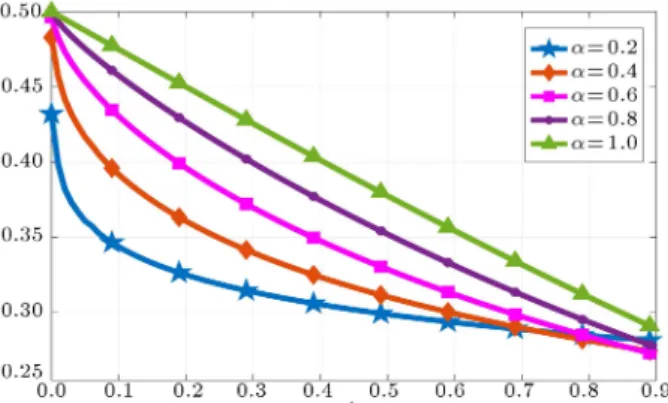
= 0: (41) This nonlinear system of equations can be solved using Newton iteration method and the vector of unknown coecients C can be computed. After calculating the vector C, we can obtain the numerical solution for y(t) using Eq. (36). Figure 1 shows the EWM
solution for m0 = 80 and the exact solution for =
1. The comparison between the exact solution and
EWM solution for various values of m0 is presented
in Table 1. As can be seen in the table, even fairly
small values of k = 3 and M = 3 (m0 = 12) produce
a good approximation. As m0 increases, the absolute
error decreases to the order of E-9. EWM solution
for m0 = 80 with various fractional values of is
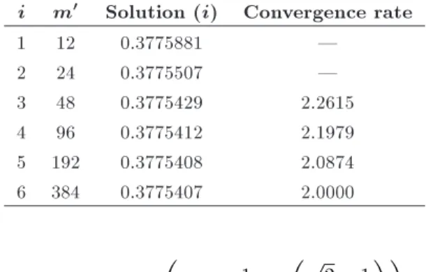
given in Figure 2. As approaches 1, the solution to the fractional-order dierential equation approaches the solution to integer-order dierential equation. The order of convergence is given in Table 2. As it is shown [41,42], this rate tends to 2.
Figure 1. The solution of EWM for = 1 and the exact solution for Example 1.
Figure 2. The solution of EWM for various values of for Example 1.
4.2. Example 2
Consider the following Riccati dierential equation: Dy(t) 2y(t) + y2(t) 1 = 0:
y(0) = 0; (42)
where 0 < 1. The exact solution for = 1 is given as:
Table 1. Comparison of the exact solution and EWM with = 1 and various values of m0 for Example 1.
t Exact solution m0= 12 m0= 24 m0 = 48 m0= 96 m0= 192 m0= 384
0.0 0.5000000 0.5000223 0.5000028 0.5000004 0.5000000 0.5000000 0.5000000 0.1 0.4750208 0.4750248 0.4750229 0.4750213 0.4750209 0.4750208 0.4750208 0.2 0.4501660 0.4501822 0.4501699 0.4501669 0.4501662 0.4501661 0.4501660 0.3 0.4255575 0.4255764 0.4255623 0.4255588 0.4255578 0.4255576 0.4255575 0.4 0.4013123 0.4013419 0.4013188 0.4013140 0.4013128 0.4013124 0.4013124 0.5 0.3775407 0.3775881 0.3775507 0.3775429 0.3775412 0.3775408 0.3775407 0.6 0.3543437 0.3543778 0.3543529 0.3543460 0.3543443 0.3543438 0.3543437 0.7 0.3318122 0.3318532 0.3318224 0.3318147 0.3318128 0.3318124 0.3318123 0.8 0.3100255 0.3100667 0.3100358 0.3100282 0.3100262 0.3100257 0.3100256 0.9 0.2890505 0.2890953 0.2890613 0.2890532 0.2890512 0.2890507 0.2890505
Table 2. The solution and convergence rate at point t = 0:5 for Example 1.
i m0 Solution (i) Convergence rate
1 12 0.3775881 |
2 24 0.3775507 |
3 48 0.3775429 2.2615
4 96 0.3775412 2.1979
5 192 0.3775408 2.0874
6 384 0.3775407 2.0000
y(t) = 1 +p2 tanh p2t +12log p
2 1 p
2 + 1 !!
: Using the same approximation as that given for Ex-ample 1 in detail, we obtain the following nonlinear equation, the solution to which produces C coecients:
CT
m0m0 2CTPm0m0m0m0
+a2
1; a22; ; a2m0
[1; 1; ; 1] = 0: (43)
where [a1; a2; ; am0] = CTPm0m0m0m0. After
nding the coecient vector C, we can again obtain the numerical solution for y(t) using Eq. (36). Figure 3 shows the solution of EWM for m0= 80 and the exact
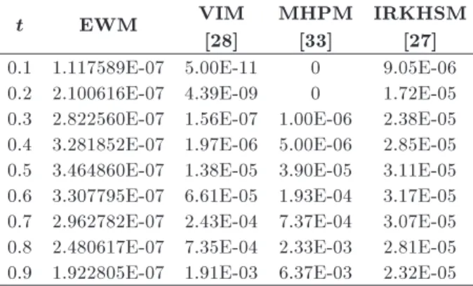
solution for = 1. The comparison between absolute errors of the EWM solution and some other solution methods for the fractional dierential equation with
various values of m0 is presented in Table 3. The
results indicate two important features; rstly, unlike in the other methods, the absolute error does not increase in the EWM as t increases and secondly, for the
m0 values greater than 96, the EWM provides better
approximation. Another comparison for = 0:75 is
given with various values of m0 in Table 4. Euler
wavelet solution for m0 = 80 with various fractional
values of is given in Figure 4. Again, it can
be stated that the solution to the fractional-order dierential equation approaches the solution to integer-order dierential equation as approaches 1.
Figure 3. The solution of EWM for = 1 and the exact solution for Example 2.
Figure 4. The solution of EWM for various values of for Example 2.
4.3. Example 3
Consider the following Riccati dierential equation: Dy(t) + y2(t) 1 = 0;
y(0) = 0; (44)
where 0 < 1. The exact solution for = 1 is given as y(t) = e2t 1
e2t+1.
Table 3. The absolute errors of EWM and some other solution methods for the fractional-order dierential equation with = 1 and various values of m0 for Example 2.
t m0= 24 m0= 48 m0= 96 m0= 192 m0= 384 MHPM [33] IRKHSM [27] OHAM [31]
0.1 5.52E-04 1.38E-04 3.43E-05 8.57E-06 2.14E-06 1.00E-06 3.58E-05 3.20E-05 0.2 6.47E-04 1.63E-04 4.06E-05 1.01E-05 2.54E-06 1.20E-05 7.58E-05 2.90E-05 0.3 7.27E-04 1.78E-04 4.46E-05 1.12E-05 2.80E-06 1.00E-06 1.20E-04 1.10E-03 0.4 7.44E-04 1.85E-04 4.56E-05 1.14E-05 2.86E-06 3.03E-04 1.66E-04 2.50E-03 0.5 5.20E-04 1.52E-04 4.07E-05 1.05E-05 2.66E-06 1.55E-03 2.12E-04 4.40E-03 0.6 5.84E-04 1.47E-04 3.78E-05 9.44E-06 2.34E-06 4.69E-03 2.52E-04 5.50E-03 0.7 4.56E-04 1.22E-04 3.05E-05 7.49E-06 1.87E-06 1.05E-02 2.87E-04 5.50E-03 0.8 3.79E-04 8.82E-05 2.22E-05 5.64E-06 1.41E-06 1.89E-02 3.40E-04 3.80E-03 0.9 2.66E-04 6.63E-05 1.60E-05 4.02E-06 1.01E-06 2.80E-02 4.90E-04 3.40E-03
Table 4. Comparison of the EWM and some other solution methods for the fractional-order dierential equation with = 0:75 for Example 2.
t m0= 24 m0= 48 m0= 96 m0= 192 m0= 384 RKM [32] MHPM [33] IRKHSM [35]
0.2 0.476341 0.475422 0.475178 0.475117 0.475117 0.4695 0.4288 0.4730 0.4 0.939340 0.938740 0.938586 0.938548 0.938548 0.9335 0.8914 0.9368 0.5 1.149579 1.149198 1.149097 1.149070 1.149070 1.1448 1.1327 1.1475 0.6 1.334765 1.334444 1.334360 1.334339 1.334339 1.3309 1.3702 1.3330 0.8 1.623300 1.623073 1.623011 1.622995 1.622995 1.6215 1.7948 1.6220
The nonlinear equation used to obtain the coe-cient vector C becomes:
CT
m0m0 [1; 1; ; 1] + [a21; a22; ; a2m0] = 0;
(45) where [a1; a2; ; am0] = CTPm0m0m0m0. As in the
other two examples, the coecient vector C is used to obtain the numerical solution for y(t) using Eq. (36).
Figure 5 presents the solution of EWM for m0 = 80
and the exact solution for = 1. The comparison between absolute errors of the Euler wavelet solution and some other solution methods for the fractional
dierential equation with m0 = 384 is provided in
Table 5. As can be seen in the table, EWM provides better approximation. Another comparison of the numerical results with = 0:75 is given for various values of m0 in Table 6.
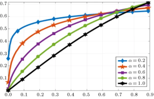
Euler wavelet solution with m0 = 80 for various
fractional values of is given in Figure 6. Again, the results show that the solution to the fractional-order
Table 5. The absolute errors of EWM and some other solution methods for the fractional-order dierential equation with = 1 for Example 3.
t EWM VIM
[28]
MHPM [33]
IRKHSM [27] 0.1 1.117589E-07 5.00E-11 0 9.05E-06 0.2 2.100616E-07 4.39E-09 0 1.72E-05 0.3 2.822560E-07 1.56E-07 1.00E-06 2.38E-05 0.4 3.281852E-07 1.97E-06 5.00E-06 2.85E-05 0.5 3.464860E-07 1.38E-05 3.90E-05 3.11E-05 0.6 3.307795E-07 6.61E-05 1.93E-04 3.17E-05 0.7 2.962782E-07 2.43E-04 7.37E-04 3.07E-05 0.8 2.480617E-07 7.35E-04 2.33E-03 2.81E-05 0.9 1.922805E-07 1.91E-03 6.37E-03 2.32E-05
dierential equation approaches the solution to integer-order dierential equation as approaches 1.
5. Conclusion
In this paper, numerical solutions to various fractional-order Riccati-type dierential equations were obtained using the Euler Wavelet Method (EWM). The opera-tional matrix of fracopera-tional integration was obtained for Euler wavelets and applied for obtaining the solution to several fractional-order Riccati dierential equations. It has been shown elsewhere that the Euler wavelets perform better than other wavelet methods [37].
The Euler Wavelet Method (EWM) results in sparse coecient matrices; therefore, it has shorter simulation duration and lower memory requirements. The numerical solutions given in detail in Section 4 proved that the EWM was a better approximation to the exact solution than other numerical solution methods when larger values of m0were used for integer
orders (corresponding to taking more samples for
dis-Figure 5. The solution of EWM for = 1 and the exact solution for Example 3.
Table 6. Comparison of the EWM and some other solution methods for the fractional-order dierential equation with = 0:75 for Example 3.
t m0= 24 m0= 48 m0= 96 m0= 192 m0= 384 RKM
[32]
Method in [30]
MHPM [33]
IRKHSM [35] 0.2 0.309815 0.309924 0.309962 0.309972 0.309972 0.3073 0.3099 0.3138 0.3100 0.4 0.481539 0.481609 0.488162 0.481630 0.481630 0.4803 0.4816 0.4929 0.4816 0.6 0.5977565 0.597762 0.597780 0.597782 0.597782 0.5975 0.5977 0.5974 0.5978 0.8 0.6788444 0.678850 0.6788495 0.678850 0.678850 0.6796 0.6788 0.6604 0.6788
Figure 6. The solution of EWM for various values of for Example 3.
cretization). Moreover, the numerical solutions for the fractional orders showed that as approached 1, they approached those for the integer orders. The results proved that the method could be applicable to various other fractional dierential equations.
The approach used here can be applied to the related dierential equations in [43].
References
1. Colinas-Armijo, N., Di Paola, M., and Pinnola, F.P. \Fractional characteristic times and dissipated energy in fractional linear viscoelasticity", Commun. Nonlin-ear Sci. Numer. Simul., 37, pp. 14-30 (2016).
2. Rossikhin, Y.A. and Shitikova M.V. \Application of fractional calculus for dynamic problems of solid me-chanics: novel trends and recent results", Appl. Mech. Rev., 63(1), pp. 1-52 (2009).
3. Magin, R.L. and Ovadia M. \Modeling the cardiac tissue electrode interface using fractional calculus", J. Vib. Control, 14(9-10), pp. 1431-1442 (2008).
4. Sommacal, L., Melchior, P., Oustaloup, A., Cabelguen, J.M., and Ijspeert, A.J. \Fractional multi-models of the frog gastrocnemius muscle", J. Vib. Control, 14(9-10), pp. 1415-1430 (2008).
5. Baillie, R.T. \Long memory processes and fractional integration in econometrics", J. Econom., 73(1), pp. 5-59 (1996).
6. Carpinteri, A. and Mainardi, F., Fractals and Frac-tional Calculus in Continuum Mechanics, Springer-Verlag, Vien, New York (1997).
7. Lima, M.F.M., Machado, J.A.T., and Crisostomo, M. \Experimental signal analysis of robot impacts in a fractional calculus perspective", J. Adv. Comput. Intell. Intell. Inform., 11, pp. 1079-1085 (2007). 8. Chen, C. and Hsiao, C. \Haar wavelet method for
solving lumped and distributed-parameter systems", IEE P-Contr. Theor. Appl., 144(1), pp. 87-94 (1997). 9. Karimi, H., Moshiri, B., Lohmann, B., and Maralani, P. \Haar wavelet-based approach for optimal control of
second-order linear systems in time domain", J. Dyn. Control Syst., 11(2), pp. 237-252 (2005).
10. Sadek, I., Abualrub, T., and Abukhaled, M. \A computational method for solving optimal control of a system of parallel beams using Legendre wavelets", Math. Comput. Model, 45(9-10), pp. 1253-1264 (2007). 11. Babolian, E., Masouri, Z., and Hatamzadeh-Varmazyar, S. \Numerical solution of nonlinear Volterra-Fredholm integro-dierential equations via direct method using triangular functions", Comput. Math. Appl., 58(2), pp. 239-247 (2009).
12. Kajani, M. and Vencheh, A. \The Chebyshev wavelets operational matrix of integration and product opera-tion matrix", Int J. Comput. Math., 86(7), pp. 1118-1125 (2008).
13. Razzaghi, M. and Youse, S. \The Legendre wavelets operational matrix of integration", Int. J. Syst. Sci., 32(4), pp. 495-502 (2001).
14. El-Wakil, S.A., Elhanbaly, A., and Abdou, M.A. \Adomian decomposition method for solving fractional nonlinear dierential equations", Appl. Math. Com-put., 182(1), pp. 313-324 (2006).
15. Momani, S. and Odibat, Z. \Numerical approach to dierential equations of fractional order", J. Comput. Appl. Math., 207(1), pp. 96-110 (2007).
16. Das, S. \Analytical solution of a fractional diusion equation by variational iteration method", Comput. Math. Appl., 57(3), pp. 483-487 (2009).
17. Gaul, L., Klein, P., and Kemple, S. \Damping descrip-tion involving fracdescrip-tional operators", Mech. Syst. Signal Pr., 5(2), pp. 81-88 (1991).
18. Podlubny, I., Fractional Dierential Equations: An Introduction to Fractional Derivatives, Fractional Dif-ferential Equations, to Methods of Their Solution and Some of their Applications, New York, Academic Press (1999).
19. Suarez, L. and Shokooh, A. \An eigenvector expansion method for the solution of motion containing frac-tional derivatives", J. Appl. Mech., 64(3), pp. 629-635 (1997).
20. Kumar, S. \A new fractional analytical approach for treatment of a system of physical models using Laplace transform", Sci. Iran. B, 21(5), pp.1693-1699 (2014). 21. Khader, M.M. \Application of homotopy perturbation
method for solving nonlinear fractional heat-like equa-tions using Sumudu transform", Sci. Iran. B, 24(2), pp. 648-655 (2017).
22. Xu, X. and Xu, D. \Legendre wavelets method for approximate solution of fractional-order dierential equations under multi-point boundary conditions", Int. J. Comput. Math., 95(5), pp. 998-1014 (2018). 23. Wang, Y.X. and Fan, Q.B. \The second kind
Cheby-shev wavelet method for solving fractional dierential equation", Appl. Math. Comput., 218(17), pp. 8592-8601 (2012).
24. Shah, F.A. and Abass, R. \Haar wavelet operational matrix method for the numerical solution of fractional order dierential equations", Nonlinear Engin., 4(4), pp. 203-213 (2015).
25. Rahimkhani, P., Ordokhani, Y., and Babolian, E. \Numerical solution of fractional pantograph dier-ential equations by using generalized fractional-order Bernoulli wavelet", J. Comput. Appl. Math., 309(1), pp. 493-510 (2017).
26. El-Tawil, M.A., Bahnasawi, A.A., and Abdel-Naby, A. \Solving Riccati dierential equation using Ado-mian's decomposition method", Appl. Math. Comput., 157(2), pp. 503-514 (2004).
27. Sakar M. \Iterative reproducing kernel Hilbertspaces method for Riccati dierential equations", J. Comput. Appl. Math., 309, pp. 163-174 (2017).
28. Batiha, B., Noorani, M.S.M., and Hashim, I. \Applica-tion of varia\Applica-tional itera\Applica-tion method to general Riccati equation", Int. Math. Forum, 2(56), pp. 2759-2770 (2007).
29. Geng, F., Lin, Y., and Cui, M. \A piecewise varia-tional iteration method for Riccati dierential equa-tions", Comput. Math. Appl., 58(11-12), pp. 2518-2522 (2009).
30. Yuzbas, S. \Numerical solutions of fractional Riccati type dierential equations by means of the Bernstein polynomials", Appl. Math. Comput., 219(11), pp. 6328-6343 (2013).
31. Mabood, F., Ismail, A.I., and Hashim, I. \Appli-cation of optimal homotopy asymptotic method for the approximate solution of Riccati equation", Sains Malays., 42(6), pp. 863-867 (2013b).
32. Li, X.Y., Wu, B.Y., and Wang, R.T. \Reproducing kernel method for fractional Riccati dierential equa-tions", Abstr. Appl. Anal., Article ID 970967, 6 pages (2014).
33. Odibat, Z. and Momani, S. \Modied homotopy per-turbation method: application to quadratic Riccati dierential equation of fractional order", Chaos Soli-tons Fractals, 36(1), pp. 167-174 (2008).
34. Khader, M.M. \Numerical treatment for solving frac-tional Riccati dierential equation", J. Egyptian Math. Soc., 21(1), pp. 32-37 (2013).
35. Sakar, M.G., Akgul, A., and Baleanu, D. \On solu-tions of fractional Riccati dierential equasolu-tions", Adv. Dier. Equ., 39, pp. 1-10 (2017).
36. Beylkin, G., Coifman, R., and Rokhlin, V. \Fast wavelet transforms and numerical algorithms", I. Commun. Pure Appl. Math., 44(2), pp. 141-183 (1991).
37. Wang, Y. and Zhu, L. \Solving nonlinear Volterra integro-dierential equations of fractional order by using Euler wavelet method", Adv. Dier. Equ., 27, pp. 1-16 (2017).
38. He, Y. and Wang, C. \Recurrence formulae for Apostol-Bernoulli and Apostol-Euler polynomials", Adv. Dier. Equ., 209, pp. 1-16 (2012).
39. Kilicman, A. \Kronecker operational matrices for frac-tional calculus and some applications", Appl. Math. Comput., 187(1), pp. 250-265 (2007).
40. Atkinson, K.E., An Introduction to Numerical Analy-sis, Wiley, New York (1978).
41. Majak, J., Shvartsman, B., Karjust, K., Mikola, M., Haavaj oe, A., and Pohlak, M. \On the accuracy of the Haar wavelet discretization method", Compos. Part B, 80, pp. 321-327 (2015).
42. Majak, J., Pohlak, M., Karjust, K., Eerme, M., Kurnitski, J., and Shvartsman, B.S. \New higher order Haar wavelet method: Application to FGM structures", Compos. Struct., 201, pp. 71-78 (2018). 43. Tural Polat S.N. \The vector-matrix form numerical
simulations for time-derivative cellular neural net-works", Int. J. Numer. Model., 31(5), pp. 1-13 (2018).
Biography
Arzu Turan Dincel received the PhD degree in Mathematical Engineering from the Yildiz Technical
University, Istanbul, Turkey. She is currently an
Assistant Professor in the Mathematical Engineering Department of Yildiz Technical University. Some of her research interests include fractional calculus, fracture mechanics, and nite element method.