Performance of cumulative count of conforming chart with variable sampling intervals in the presence of inspection errors

(1)

Performance of cumulative count of conforming chart with

variable sampling intervals in the presence of inspection errors

Mohammad Saber Fallah Nezhad1*,Yousof Shamstabar1

1

Industrial Engineering Department, Yazd University, Iran [email protected], [email protected]

Abstract

In high quality industrial processes, the control chart is design based on cumulative count of conforming (CCC) items is very useful. In this paper, the performance of CCC-r chart with variable sampling intervals (CCC-rVSI chart) in the presence of

inspection errors is investigated. The efficiency of CCC-rVSI chart is compared with

CCC-r chart with fixed sampling interval (CCC-rFSI chart). The comparison results

show thatthe VSI scheme can performs better than the FSI scheme. In addition, analysis and discussion of the results are presented to illustrate the effect of input parameters on the performance of CCC-rVSI chart.

Keywords: high quality processes; CCC-r chart; variable sampling interval; inspections errors; average time to signal

1- Introduction

As one of the basic Statistical Process Control (SPC) tools, control chart is useful in maintaining stability and improving quality through variability reduction in the production process. The cumulative count of conforming (CCC) control chart is based on the cumulative number of conforming items between two consecutive nonconforming items that is the random variable with the geometric distribution (Calvin, 1983; Goh, 1987).This control chart is mostly applied for high- quality processes. In the automated and discrete manufacturing systems, very low level of non-conforming items is produced. As a result the CCC chart has received considerable attention from the industry (Joekes et al., 2016).The CCC-r chaCCC-rt is developed based on the CCC chaCCC-rt which consideCCC-rs the cumulative count of confoCCC-rming items until observing a fixed number ''r'' of nonconforming ones that follows the negative binomial distribution(Ohta et al.,2001; Kudo et al.,2004).

The scheme of variable sampling interval (VSI) is designed in order to improve the efficiency of the CCC control chart (Liuet al., 2006).The current researches on the application of VSI scheme have denoted the better performance of this scheme in comparison with FSI scheme.X control chart with variable sampling intervals was proposed by some researchers (see for example, Reynolds et al.,1988; Reynolds and Arnold , 1989; Runger and Pignatiello Jr, 1991; Runger and Montgomery, 1993; Amin and Miller, 1993; Zhang et al.,2012). Aparisi and Haro, (2001) and Villalobos et al. (2005) studied a VSI multivariate shewhart chart. Reynolds et al., (1990) and Luo and Wang (2009) investigated the VSI- CUSUM control chart. VSI- EWMA charts have been studied by some researchers (see for example, Shamma et al., 1991; Saccucci et al, 1992;Castagliolaet al, 2006; Castagliolaet et al, 2006).

*Corresponding author.

Vol. 10, special issue on Quality Control and Reliability, pp.78 – 92 Winter (February) 2017

(2)

Some studies have been performed for VSI- CCC (CCCVSI) chart and they concluded that their

proposed design is more efficient than FSI- CCC (CCCFSI chart). First, Liu et al. (2006) proposed CCC

chart with variable sampling intervals (CCCVSI chart). Chen et al. (2011) investigated CCC chart with

variable sampling intervals and variable control limits (CCCVSI/VCL chart) and Chen (2013) studied CCC

chart with variable sampling intervals for correlated samples (GCCCVSI chart). Zhang et al. (2014)

investigated the performance of CCCVSI chart with estimated control limits.

The strategy of using 100% inspection is proposed for the implementation of the CCC chart and many studies on this charts have assumed that inspection is perfect accurate, but inspection errors exist in the process. Burke et al.(1995) discussed inspection errors and their impact on control charts and denoted their important effect on the results. Lu et al. (2000) calculated the adjusted control limits for the CCC chart in the presence of inspection errors based on the relationship between the true and observed values of the nonconforming proportion. Ranjan et al. (2003) designed a procedure to set control limits for CCC charts considering the inspection errors to obtain the maximum ARL. Some other studies about inspection errors have been done by Case (1980), Lindsay (1985), Suich (1988),Huang et al. (1989), Suich (1990), Johnson et al.(1991), Cheng and Chung(1994), Wang and Chen (1997, Ryan (2011), Nezhad and Nasab (2012) , Fallahnezhad and Babadi(2015) and Fallah Nezhad et al.(2015).

The goal of this paper is to develop a model to consider the inspection errors in implementation of variable sampling interval scheme for CCC-r control chart. So, this paper considers the adjusted control limits for the CCC-rVSI chart that can reduce for the effects of inspection errors. In section 2, the CCC-r

VSI Chart in the presence of inspection errorshas been described .In section 3, the comparison study

between the CCC-rVSI chart and the CCC-rFSI chart is performed and the results are elaborated using

sensitivity analysis. In section 4, a practical case study for the implementation of the CCC-rVSI chart in the

presence of inspection errors is described. Finally, we have concluded the paper.

2- Description of the CCC-r

VSI

chart

2-1- Notations

0t

p

the observed value of the in-control nonconforming fraction,

1t

p

the observed value of the out-of-control nonconforming fraction,

0

p

the true value of the in-control nonconforming fraction, 1

p

the true value of the out-of-control nonconforming fraction,

disired

α

the probability of false alarm,

i

X

the cumulative count of items inspected after observing the (i-1)th nonconforming item until the

ith nonconforming item (including the last nonconforming item),

n the number of different intervals for the CCC-rVSI chart,

j

d

j =1,2,…,n. Sampling interval lengths for the CCC-rVSI chart, , i.e., the time between inspections

of two consecutive items (dn<dn-1<…<d2<d1)

d

the sampling interval length for the CCC-rFSI chart,

(3)

LCL into n sub-regions I I₁; ₂; .. . ; I_n

(

IL_n₋₁<IL_n₋₂< … <IL₁

)

, Li the sampling interval length which is used to obtain Xi,

ARLa a

ATS

the adjusted average run length, the _{adjusted average time to signal,}

ATSaV the adjusted in-control ATS of the CCC-rVSI chart,

ATSaF the adjusted in-control ATS of the CCC-rFSI chart, '

aV

ATS

the adjusted out-of-control ATS of the CCC-rVSI chart,

aF

ATS

′

the adjusted out-of-control ATS of the CCC-rFSI chart,

I _{improvement factor, defined as} ' '

/

V F

I

=

ATS

_,

j

q

the probability that point Xi falls region I_j when the process nonconforming fraction is p0 ,

j

q

′

the probability that point Xi falls within the regionIjwhen the process nonconforming fraction is

1 p

2-2- CCC-rVSI control chart in the presence of the inspection errors

The relationship between the true and observed value of nonconforming proportion in presence of inspection errors is as follows (Burke et al., 1995):

(

1

2

)

(

1 )

1

t t

p

=

p

−

e

+ −

p e

(1)

The observed (estimated) non-conforming fraction is

p

_t and

p

is the true value of nonconforming proportion, while ( ) and ( ) denote, respectively, the probability of classifying a conforming item as nonconforming and the probability of classifying a nonconforming item as conforming. So, we have:

in control state:

p

₀

=

p

₀_t

(

1 −

e

₂

)

+ −

(

1 p

₀_t

)

e

₁

out of control state:

p

₁

=

p

₁_t

(

1 −

e

₂

)

+ −

(

1 p

₁_t

)

e

₁

If the acceptable risk of false alarm is

α

desired , then the control limits and the center line can be

determined as follows (Xie et al., 2012):

1

0 0

1 (1

)

1 / 2

1

UCL

i r r

t t disired

i r

i

p

r

α

−

− =

−





−

= −



₋







∑

(2)

(4)

0 0

1 (1

)

0.5

1

CL

i r r

t t i r

i

p

r

− =

−





−

=



₋







∑

(3)

(4)

Lu et al. (2000) proposed the adjusted acceptable risk of false alarm in the presence of inspection errors. Thus a control chart is modified to provide a first type error that is closer to the one under error-free inspection in order to reduce the impact of inspection errors. In the presence of inspection errors, can be obtained as following,

∗ ₌ (5)

As the result, in the presence of inspection errors, the adjusted control limits and the center line can be determined as follows:

1

0 0

1 (1

)

1 / 2

1

a

UCL

i r r

disired i r

i

p

r

α

− − ∗ =

−





−

= −



₋







∑

(6) 0 0

1 (1

)

0.5

1

a

CL

i r r i r

i

p

r

− =

−





−

=





−





∑

(7) (8)

The ARL (average run length) is defined as the average number of points plotted until receiving an out-of-control signal. Thus,

ARL

_acan be obtained as following,

1

1 (1

)

1

a

a UCL

r i r

LCL

ARL

i

p

r

−

=

₋





−



₋



−





∑

(9)

ANI (average number of items) is defined as the expected value of the number of items inspected until the chart signals an alarm .ANIa can be computed for CCCG-rFSI and CCCG-rVSI chart by applying the

following equation:

a a

r

ANI ARL

p

= (10)

When the CCC-rVSI chart is applied, then the time between inspections of two consecutive items would be

1 2 n 1 2 n

d , d , . . . , d (d > d > . . . >d ). These interval lengths should be determined considering the

0 0

1 (1

)

/ 2

1

LCL

i r r

t t desired

i r

i

p

r

α

− =

−





−

=



₋







∑

0 0

1 (1

)

/ 2

1

a LCL

i r r

desired i r

i

p

r

α

− ∗ =

−





−

=



₋







∑

(5)

practical conditions of production system. As an example, the minimum value of interval length is not less than the time lag between productions of two successive items. The maximum value of interval length can be obtained with regards to the maximum amount of time that is allowed for the process to run without inspection. The interval limits IL1,IL2, . . . ,ILn are determined in the CCC-rVSI chart, so that the

interval between UCLa and LCLa is divided into n different intervals I1, I2, . . . , In. Thus following

framework is used for sampling from the process,

1 1 1 1

2 1 2 2 1

1

, X

(

,

)

, X

(

,

)

.

, X

(L

,

)

i a

i

n i n a n

d

I

IL UCL

d

I

IL IL

L

d

I

CL IL

− −

−

∈ =





_{∈ =}





=





∈ =



(11)

The interval limits IL IL1, 2, .. . , ILn−1can be determined as the following that F -1

is inverse function of the negative binomial distribution function with r and p0 parameters :

= ( + 1 ≤ < ) = ( ≥ + 1) − ( ≥ )

= # $ − 1_{− 1%}

& '()*+,

(1 − )'- _{− # $ − 1}

− 1% (1 − )

'-& '(./*

= # $ − 1_{− 1%}

./*-'()*+,

(1 − )'- _{= 1 − 0( ) −} ∗

2

= 0- _{(1 − −} ∗

2 )

So we have:

= 0- _{(1 − −} ∗

2 )

= 0- _{21 − − −} ∗

2 3

. . .

4- = 0- (1 − − − ⋯ − 4 −

∗ 2 )

(6)

This scheme continues until the IL values falls between UCLa and LCLaas following:

(13)

ATS is the average length of time that is needed to observe a signal in a control chart. Also, ATSaF and

ATSaV can be determined as following,

a F a a

r

ATS

ANI

d

ARL

d

p

=

× =

× ×

(14)

1 1 2 2

1 2

....

n n

aV a

n

r

d q

ATS

ARL

p

q

+

+ +

=

× ×

+ + +

(15)

3- Performance comparisons between the CCC-r

VSI

and the CCC-r

FSI

chart

The performance of CCC-rVSIis compared with the CCC-rFSI chart in this section. Note that the same

values of nonconforming fraction p0 and false alarm probability

α

are assumed for both the CCCFSI and

the CCCVSI chart. In order to compare these charts, the design parameters for the CCC-rVSI and the

CCC-rFSI chart are determined so that the equation ATSaF = ATSaV is satisfied at the in control state. On the

other hand, when the process nonconforming fraction changes to

p

₁

( p )

>

₀ , the values of

ATS

'_aF and

'

aV

ATS

should be evaluated. The control chart with smaller value of out-of-control

ATS

'_awill have the better performance.

Let

ATS

_aF =

ATS

_aV, thus,

1 1 2 2 1 1 2 2

1 2

....

1

n n n n

n

d q

d

q

α

+

+ +

+

+ +

=

+ + +

−

(16)

It is assumed that the sampling interval length of the CCC-rFSI chart is adjusted to be equal 1 ( d = 1), the

values of

(

d₁, d₂, . . . ,d_n

)

and

(

q₁, q₂, . . . ,q_n

)

are determined so that Eq. (16) is satisfied then the matched CCC-rVSI and CCC-rFSI chart are obtained that have the same in-control value of ATS. Then,

when the nonconforming fraction changes to

p

₁, the performance of the CCC-rVSI chart can be analyzed

by computing the value of I, that is equal to the ratio of out-of-control ATSa of the CCC-rVSI and the

CCC-rFSI chart:

' ' ' '

1 1 2 2

' ' ' '

1 2

....

aV n n

aF n

ATS

d q

I

ATS

q

+

+ +

=

+

+ +

(17)

Based on Equation (17), if the value of Improvement factor is less than 1.00, variable sampling interval scheme can produce a signal more quickly than fixed sampling interval scheme when the process is out of control. So, when Iis less than 1.00, it denotes that the CCC-rVSI chart performs better than the CCC-rFSI

chart.

The values of

q

'_j can be calculated as following,

1 2 ... 2 1

a n n a

(7)

(18)

The performance of CCC-rVSI chart is analyzed based on the number of sampling interval (n) assuming

equal probabilities for each interval:

1 2

1 ...

_n

q

n

α

−

= = = =

(19)

By substituting d=1 in Equation (16), we have,

1 1 2 2 1 2

1

1 d q

d q

....

d q

_n _n

(

d

...

d

_n

)

n

α

−

− =

+

+ +

=

+ + +

1 2

...

n

d

+

d

+ +

d

=

n

(20)

4- Comparative study of CCC-r

VSI

chart in the presence of inspection errors

In this paper, we apply the input data in the numerical study of Liu et.al (2006)for comparison study. This data is as following:

α

disired

=

0.0027,

p

0t

=

0.0005

and sampling interval lengths

(d ,

1

d

2

,...,

d

n

)

with the fixed value ofd =1can be chosen as follows:

1 2 1 2 3 1 2 3 4

1 2 3 4 5

2, 1.9, 0.1; 3, 1.9, 1, 0.1; n 4, d 1.9, 1.2, 0.8, 0.1; n 5, d 1.9, 1.5, 1, 0.5, d 0.1;...

n d d n d d d d d d

d d d

= = = = = = = = = = = =

= = = = = =

4-1- Improvement factors for different process shifts

Now, we study the performance of CCC-rVSI chart in the presence of inspection errors for different

value of process shifts and several values of e1 and e2.First, the value of corresponding improvement

1 1 2 2 1 1 1

1 1 1

1

2 1 1

1

1 1 1

1 1 1 1

1 (1

)

1

1 (1

)

1 .

.

1 (1

)

1

1 (1

)

1

a n n n a UCL

r x r

x IL IL

r x r

x IL

IL

r x r

n

x IL IL

r x r

n

x LCL

x

q

p

r

x

q

p

r

x

q

p

r

x

q

p

r

− − − − − = + − = + − − = + − = +





₋



′ =

−







−







_

₋

_

′



₌

_

_

₋

−

















₋



′ =

−





₋









_

₋

_



_{′ =}

_

_

₋

−









∑

(8)

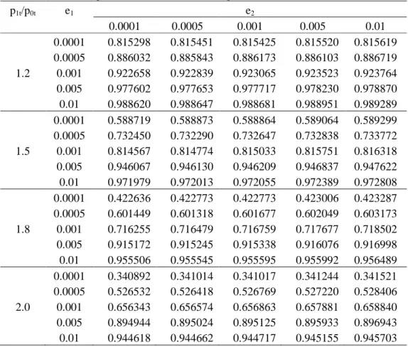
factors I are computed and the results are shown in Table 1. As can be seen when the nonconforming ratio (p1t/p0t) increases then, the improvement factor I decreases, and thus the CCC-rVSI chart performs better

than CCC-rFSI chart in the presence of the inspection errors.

Table 1. Improvement factors for different process shifts with n=2 and r=3

p1t/p0t e1 e2

0.0001 0.0005 0.001 0.005 0.01 0.0001 0.815298 0.815451 0.815425 0.815520 0.815619

0.0005 0.886032 0.885843 0.886173 0.886103 0.886719 1.2 0.001 0.922658 0.922839 0.923065 0.923523 0.923764 0.005 0.977602 0.977653 0.977717 0.978230 0.978870 0.01 0.988620 0.988647 0.988681 0.988951 0.989289 0.0001 0.588719 0.588873 0.588864 0.589064 0.589299 0.0005 0.732450 0.732290 0.732647 0.732838 0.733772 1.5 0.001 0.814567 0.814774 0.815033 0.815751 0.816318 0.005 0.946067 0.946130 0.946209 0.946837 0.947622 0.01 0.971979 0.972013 0.972055 0.972389 0.972808 0.0001 0.422636 0.422773 0.422773 0.423006 0.423287 0.0005 0.601449 0.601318 0.601677 0.602049 0.603173 1.8 0.001 0.716255 0.716479 0.716759 0.717677 0.718502 0.005 0.915172 0.915245 0.915338 0.916076 0.916998 0.01 0.955506 0.955545 0.955595 0.955992 0.956489 0.0001 0.340892 0.341014 0.341017 0.341244 0.341521 0.0005 0.526532 0.526418 0.526769 0.527220 0.528406 2.0 0.001 0.656343 0.656574 0.656863 0.657881 0.658840 0.005 0.894944 0.895024 0.895125 0.895933 0.896943 0.01 0.944618 0.944662 0.944717 0.945155 0.945703

When e1 (the probability of classifying a nonconforming item as conforming) increaseas, the

improvement factor I also increseas and with increasing e2, the value of improvement factor increases.

Thus it is concluded that the superiority of CCC-rVSI chart over CCC-rFSI chart improves by increasing the

enspection errors.

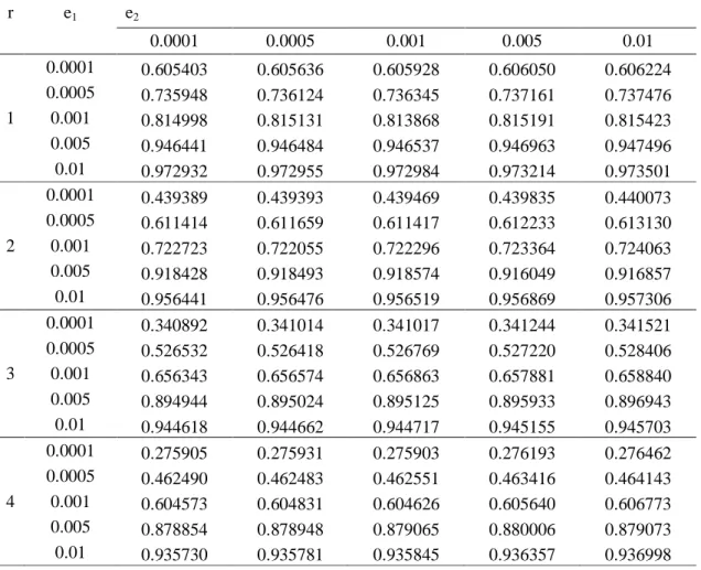
4-2- Improvement factors for different CCC-rVSI control chart

In this subsection, we fix the number of sampling intervals (n=2), and process shift (p1t/p0t=2) then for

different possible values of parameter r, the results are shown in Table 2. The improvement factor decreases by increasing the parameter r in the all cases.

(9)

Table 2. Improvement factors for different CCC-rVSI control chart with n=2 and (p1t/p0t=2) r e1 e2

0.0001 0.0005 0.001 0.005 0.01 0.0001 0.605403 0.605636 0.605928 0.606050 0.606224 0.0005 0.735948 0.736124 0.736345 0.737161 0.737476 1 0.001 0.814998 0.815131 0.813868 0.815191 0.815423 0.005 0.946441 0.946484 0.946537 0.946963 0.947496 0.01 0.972932 0.972955 0.972984 0.973214 0.973501 0.0001 0.439389 0.439393 0.439469 0.439835 0.440073 0.0005 0.611414 0.611659 0.611417 0.612233 0.613130 2 0.001 0.722723 0.722055 0.722296 0.723364 0.724063 0.005 0.918428 0.918493 0.918574 0.916049 0.916857 0.01 0.956441 0.956476 0.956519 0.956869 0.957306 0.0001 0.340892 0.341014 0.341017 0.341244 0.341521 0.0005 0.526532 0.526418 0.526769 0.527220 0.528406 3 0.001 0.656343 0.656574 0.656863 0.657881 0.658840 0.005 0.894944 0.895024 0.895125 0.895933 0.896943 0.01 0.944618 0.944662 0.944717 0.945155 0.945703 0.0001 0.275905 0.275931 0.275903 0.276193 0.276462 0.0005 0.462490 0.462483 0.462551 0.463416 0.464143 4 0.001 0.604573 0.604831 0.604626 0.605640 0.606773 0.005 0.878854 0.878948 0.879065 0.880006 0.879073 0.01 0.935730 0.935781 0.935845 0.936357 0.936998

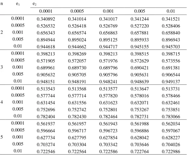
4-3-Improvement factors for different numbers of sampling intervals

In order to investigate the overall performance of CCC-rVSI chart based on the number of sampling

intervals, we fix the parameter r=3, and process shifts (p1t/p0t) = 2. The results in Table 3 indicate that for

different values of e1 and e2, the number of sampling intervals is efficient on the improvement factor, I.

for example, if e1=0.0001 and e2=0.0001, then CCC-r VSI chart with n=2, is more efficient and if e1=0.005

(10)

Table 3. Improvement factors for different numbers of sampling intervals with r=3 and p1t/p0t=2 n e1 e2

0.0001 0.0005 0.001 0.005 0.01 0.0001 0.340892 0.341014 0.341017 0.341244 0.341521 0.0005 0.526532 0.526418 0.526769 0.527220 0.528406 2 0.001 0.656343 0.656574 0.656863 0.657881 0.658840 0.005 0.894944 0.895024 0.895125 0.895933 0.896943 0.01 0.944618 0.944662 0.944717 0.945155 0.945703 0.0001 0.398213 0.398269 0.398213 0.398515 0.398715 0.0005 _0.571905 _0.572057 _0.571976 _0.572629 _0.573556 3 0.001 _0.689961 _0.689730 _0.689796 _0.690421 _0.691381 0.005 _0.905632 _0.905705 _0.905796 _0.905631 _0.906544 0.01 0.948151 0.948191 0.948241 0.948639 0.949137 0.0001 0.513543 0.513568 0.513577 0.513647 0.513731 0.0005 0.577744 0.577714 0.577820 0.578016 0.578466 4 0.001 0.631454 0.631556 0.631623 0.632071 0.632461 0.005 0.752696 0.752742 0.752801 0.753267 0.753851 0.01 0.782404 0.782430 0.782464 0.782731 0.783066 0.0001 0.561937 0.561957 0.561943 0.561988 0.562034 0.0005 _0.596664 _0.596717 _0.596723 _0.596886 _0.597067 5 0.001 _0.627734 _0.627795 _0.627854 _0.628042 _0.628227 0.005 _0.703274 _0.703304 _0.703342 _0.703646 _0.704026 0.01 0.722546 0.722564 0.722586 0.722764 0.722986

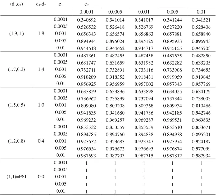
4-4- Improvement factors based on different lengths of sampling interval

Based on the above analysis, we investigate the effect of interval length on the performance of CCC-rVSI

chart when the number of sampling intervals is n=2.Four different cases of sampling interval lengths are analyzed. As can be seen in Table 4 the larger values for the differences between interval lengths, (d1, d2)

leads to better performance of CCC-rVSI chart. Also, in all cases, the value of I is less than 1, thus the

(11)

Table 4. Improvement factors based on different lengths of sampling interval with n=2 ,r=3 and p1t/p0t=2 (d1,d2) d1-d2 e1 e2

0.0001 0.0005 0.001 0.005 0.01 0.0001 _0.340892 _0.341014 _0.341017 _0.341244 _0.341521 0.0005 _0.526532 _0.526418 _0.526769 _0.527220 _0.528406 (1.9,.1) 1.8 0.001 0.656343 0.656574 0.656863 0.657881 0.658840 0.005 0.894944 0.895024 0.895125 0.895933 0.896943 0.01 0.944618 0.944662 0.944717 0.945155 0.945703 0.0001 0.487361 0.487455 0.487458 0.487635 0.487850 0.0005 _0.631747 _0.631659 _0.631932 _0.632282 _0.633205 (1.7,0.3) 1.4 0.001 0.732711 0.732891 0.733116 0.733908 0.734653 0.005 0.918289 0.918352 0.918431 0.919059 0.919845 0.01 0.956925 0.956959 0.957002 0.957343 0.957769 0.0001 _0.633829 _0.633896 _0.633898 _0.634025 _0.634179 0.0005 0.736962 0.736899 0.737094 0.737344 0.738003 (1.5,0.5) 1.0 0.001 0.809080 0.809208 0.809368 0.809934 0.810466 0.005 0.941635 0.941680 0.941736 0.942185 0.942746 0.01 0.969232 0.969257 0.969287 0.969531 0.969835 0.0001 0.853532 0.853559 0.853559 0.853610 0.853671 0.0005 0.894785 0.894760 0.894838 0.894938 0.895201 (1.2,0.8) 0.4 0.001 0.923632 0.923683 0.923747 0.923974 0.924187 0.005 0.976654 0.976672 0.976695 0.976874 0.977099 0.01 0.987693 0.987703 0.987715 0.987812 0.987934

0.0001 1 1 1 1 1

0.0005 1 1 1 1 1

(1,1)=FSI 0.0 0.001 1 1 1 1 1

0.005 1 1 1 1 1

0.01 1 1 1 1 1

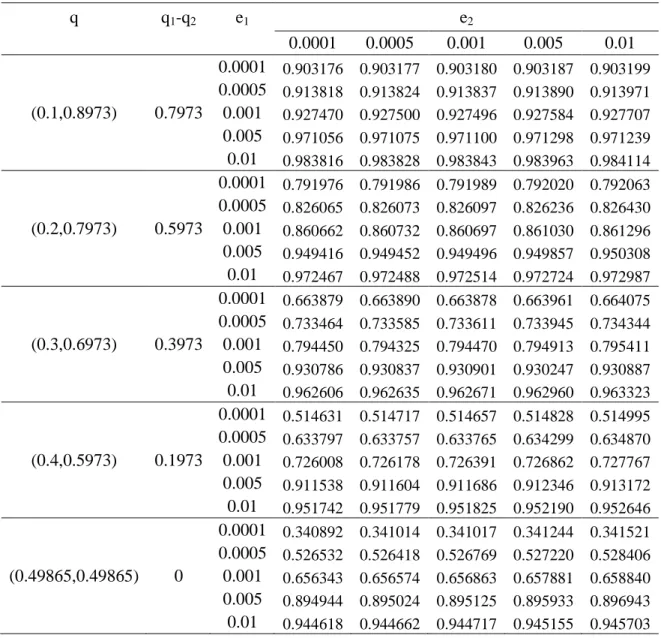
4-5- Improvement factors for different probability allocations

The above overall performance of CCC-rVSI chart is analyzed based on the equal in control probability

allocations. In order to investigate the overall performance of CCC-rVSI chart when the condition

q1 = q2 = ⋯ = qn is not satisfied, we fix n=2 and d1=1.9, and only change the values of in control

probability, q1 as proposed by Liu et al. (2006). It should be noted that q1+q2=1-α. The value of d2 can be

obtained using the following equation:

(21)

As shown in Table 5, when (q1-q2) decreases, improvement factor 1 decreases and the performance of

CCC-rVSI chart in the presence of the inspection errors becomes better. 1 1

2

2 1

0 d q d

q

α

− − = >

(12)

Table 5. Improvement factors for different probability allocations with n=2, r=3 and p1t/p0t=2

q q1-q2 e1 e2

0.0001 0.0005 0.001 0.005 0.01 0.0001 0.903176 0.903177 0.903180 0.903187 0.903199

0.0005 0.913818 0.913824 0.913837 0.913890 0.913971

(0.1,0.8973) 0.7973 0.001 0.927470 0.927500 0.927496 0.927584 0.927707

0.005 0.971056 0.971075 0.971100 0.971298 0.971239

0.01 0.983816 0.983828 0.983843 0.983963 0.984114

0.0001 0.791976 0.791986 0.791989 0.792020 0.792063

0.0005 0.826065 0.826073 0.826097 0.826236 0.826430

(0.2,0.7973) 0.5973 0.001 0.860662 0.860732 0.860697 0.861030 0.861296

0.005 0.949416 0.949452 0.949496 0.949857 0.950308

0.01 0.972467 0.972488 0.972514 0.972724 0.972987

0.0001 0.663879 0.663890 0.663878 0.663961 0.664075

0.0005 0.733464 0.733585 0.733611 0.733945 0.734344

(0.3,0.6973) 0.3973 0.001 0.794450 0.794325 0.794470 0.794913 0.795411

0.005 0.930786 0.930837 0.930901 0.930247 0.930887

0.01 0.962606 0.962635 0.962671 0.962960 0.963323

0.0001 0.514631 0.514717 0.514657 0.514828 0.514995

0.0005 0.633797 0.633757 0.633765 0.634299 0.634870

(0.4,0.5973) 0.1973 0.001 0.726008 0.726178 0.726391 0.726862 0.727767

0.005 0.911538 0.911604 0.911686 0.912346 0.913172

0.01 0.951742 0.951779 0.951825 0.952190 0.952646

0.0001 0.340892 0.341014 0.341017 0.341244 0.341521

0.0005 0.526532 0.526418 0.526769 0.527220 0.528406

(0.49865,0.49865) 0 0.001 0.656343 0.656574 0.656863 0.657881 0.658840

0.005 0.894944 0.895024 0.895125 0.895933 0.896943

0.01 0.944618 0.944662 0.944717 0.945155 0.945703

5- Conclusion

In manufacturing technology, many production processes today are producing a very small proportion of nonconforming items. Thus, many process control methods have been proposed, such as CCC chart that has received considerable attention from the industry. In this paper, we have investigated the performance of CCC-rVSI control chart in the presence of the inspection errors for high quality processes.

Some sensitivity analysis was done and the results demonstrated that the CCC-rVSI chart is more efficient

than CCC-rFSI chart and when the parameter r increases then, the efficiency of CCC-rVSI chart will be

enhanced. Also the superiority of CCC-rVSI increases by increasing the difference between the interval

lengths and uniform probability allocation is more efficient. For future woks, we suggested developing the CCC-r chart with the variable sampling intervals under group inspection in the presence of inspection errors.

(13)

References

Amin, R. W., & Miller, R. W. (1993). A robustness study of X charts with variable sampling intervals. Journal of Quality Technology, 25, 36-36.

Aparisi, F., & Haro, C. L. (2001). Hotelling's T2 control chart with variable sampling intervals. International Journal of Production Research, 39(14), 3127-3140.

Burke, R. J., Davis, R. D., Kaminsky, F. C., & Roberts, A. E. (1995). The effect of inspector errors on the true fraction non-conforming: an industrial experiment. Quality Engineering, 7(3), 543-550.

Calvin, T. (1983). Quality Control Techniques for" Zero Defects". IEEE Transactions on Components, Hybrids, and Manufacturing Technology, 6(3), 323-328.

Case, K. E. (1980). The p control chart under inspection error. Journal of Quality Technology, 12(1), 1-9. Castagliola, P., Celano, G., & Fichera, S. (2006). Evaluation of the statistical performance of a variable sampling interval R EWMA control chart. Quality Technology & Quantitative Management, 3(3), 307-323.

Castagliola, P., Celano, G., Fichera, S., & Giuffrida, F. (2006). A variable sampling interval S2-EWMA control chart for monitoring the process variance. International Journal of Technology Management, 37(1-2), 125-146.

Chen, S.-L., & Chung, K.-J. (1994). Inspection error effects on economic selection of target value for a production process. European Journal of Operational Research, 79(2), 311-324.

Chen, Y.-K. (2013). Cumulative conformance count charts with variable sampling intervals for correlated samples. Computers & Industrial Engineering, 64(1), 302-308.

Chen, Y. K., Chen, C. Y., & Chiou, K. C. (2011). Cumulative conformance count chart with variable sampling intervals and control limits. Applied stochastic models in business and industry, 27(4), 410-420. Fallahnezhad, M., & Babadi, A. Y. (2015). A New Acceptance Sampling Plan Using Bayesian approach in the presence of inspection errors. Transactions of the Institute of Measurement and Control, 37(9), 1060-1073.

Fallah Nezhad, M. S., Yousefi Babadi, A., Owlia, M. S., & Mostafaeipour, A. (2015). A recursive Approach for lot Sentencing problem in the Presence of inspection errors. Communications in Statistics-Simulation and Computation, (just-accepted), 00-00.

Goh, T. (1987). A control chart for very high yield processes. Quality Assurance, 13(1), 18-22. Huang, Q., Johnson, N. L., & Kotz, S. (1989). Modified Dorfman-Sterrett screening (group testing) procedures and the effects of faulty inspection. Communications in Statistics-Theory and Methods, 18(4), 1485-1495.

Joekes, S., Smrekar, M., & Righetti, A. F. (2016). A comparative study of two proposed CCC-r charts for high quality processes and their application to an injection molding process. Quality Engineering, 1-9.

(14)

Johnson, N. L., Kotz, S., & Wu, X.-Z. (1991). Inspection errors for attributes in quality control (Vol. 44): CRC Press.

Kudo, K., Ohta, H., & Kusukawa, E. (2004). Economic Design of A Dynamic CCC–r Chart for High-Yield Processes. Economic Quality Control, 19(1), 7-21.

Lindsay, B. G. (1985). Errors in inspection: integer parameter maximum likelihood in a finite population. Journal of the American Statistical Association, 80(392), 879-885.

Liu, J., Xie, M., Goh, T., Liu, Q., & Yang, Z. (2006). Cumulative count of conforming chart with variable sampling intervals. International Journal of Production Economics, 101(2), 286-297.

Lu, X., Xie, M., & Goh, T. (2000). An investigation of the effects of inspection errors on the run-length control charts. Communications in Statistics-simulation and Computation, 29(1), 315-335.

Luo, Y., Li, Z., & Wang, Z. (2009). Adaptive CUSUM control chart with variable sampling intervals. Computational Statistics & Data Analysis, 53(7), 2693-2701.

Nezhad, M. F., & Nasab, H. H. (2012). A new Bayesian acceptance sampling plan considering inspection errors. Scientia Iranica, 19(6), 1865-1869.

Ohta, H., Kusukawa, E., & Rahim, A. (2001). A CCC‐r chart for high‐yield processes. Quality and Reliability Engineering International, 17(6), 439-446.

Ranjan, P., Xie, M., & Goh, T. (2003). Optimal control limits for CCC charts in the presence of inspection errors. Quality and Reliability Engineering International, 19(2), 149-160.

Reynolds Jr, M. R., & Arnold, J. C. (1989). Optimal one-sided Shewhart control charts with variable sampling intervals. Sequential Analysis, 8(1), 51-77.

Reynolds, M. R., Amin, R. W., & Arnold, J. C. (1990). CUSUM charts with variable sampling intervals. Technometrics, 32(4), 371-384.

Reynolds, M. R., Amin, R. W., Arnold, J. C., & Nachlas, J. A. (1988). Charts with variable sampling intervals. Technometrics, 30(2), 181-192.

Runger, G.C., & Montgomery,D. (1993). Adaptive sampling enhancements for Shewhart control charts. IIE transactions, 25(3), 41-51.

Runger, G. C., & Pignatiello Jr, J. J. (1991). Adaptive sampling for process control. Journal of Quality Technology, 23(2), 135-155.

Ryan, T. P. (2011). Statistical methods for quality improvement: John Wiley & Sons.

Saccucci, M. S., Amin, R. W., & Lucas, J. M. (1992). Exponentially weighted moving average control schemes with variable sampling intervals. Communications in Statistics-simulation and Computation, 21(3), 627-657.

Shamma, S. E., Amin, R. W., & Shamma, A. K. (1991). A double exponentially weigiited moving average control procedure with variable sampling intervals. Communications in Statistics-simulation and Computation, 20(2-3), 511-528.

(15)

Suich, R. (1988). The c control chart under inspection error. Journal of Quality Technology, 20(4), 263-266.

Suich, R. (1990). The effects of inspection errors on acceptance sampling for nonconformities. Journal of Quality Technology, 22(4), 314-318.

Villalobos, J. R., Muñoz, L., & Gutierrez, M. A. (2005). Using fixed and adaptive multivariate SPC charts for online SMD assembly monitoring. International Journal of Production Economics, 95(1), 109-121. Wang, R.-C., & Chen, C.-H. (1997). Minimum average fraction inspected for continuous sampling plan CSP-1 under inspection error. Journal of Applied Statistics, 24(5), 539-548.

Xie, M., Goh, T. N., & Kuralmani, V. (2012). Statistical models and control charts for high-quality processes: Springer Science & Business Media.

Zhang, M., Nie, G., & He, Z. (2014). Performance of cumulative count of conforming chart of variable sampling intervals with estimated control limits. International Journal of Production Economics, 150, 114-124.

Zhang, Y., Castagliola, P., Wu, Z., & Khoo, M. B. (2012). The variable sampling interval X chart with estimated parameters. Quality and Reliability Engineering International, 28(1), 19-34.