KIRBY N. SMITH: Computer Modeling of Contaminant Jet
Flow into Local Exhaust Hoods. (Under the direction of
Assistant Professor, Michael R. Flynn, Sc.D.).
A computer model was developed and coded in BASIC to
predict the streamline that a jet of gaseous sulfur
hexafluoride will follow in the flow field of a flanged
circular exhaust hood (FCH). This approximate solution
is based on the vector addition of a modified potential
flow solution for the FCH, and a jet flow solution. The
assumptions underlying the equations describing jet flow
are those of the Prandtl mixing length hypothesis. The
computer program generates streamlines for the combined
flow by means of iterative vector addition. The
interactive program prompts the user for the hood and jet
diameters and flows, and the distance from the hood at
which the jet is placed. A graphic plot of the predicted
streamline followed by the gas jet is displayed.
The program is used to predict the critical distance
[Z/D]5Q, the distance along the hood centerline (Z), as a
fraction of the hood diameter (D), where the jet can be
placed such that 50% of the jet contaminant flow is
captured. A series of such [Z/DJ^q values was generated
The program was validated in the laboratory. A
probe was placed in the duct of a flanged circular
exhaust hood and was connected to an electron-capture gas
chromatograph, to determine the concentration of SFg in
the hood. Capture efficiencies (ratios of "captured" gas
concentrations at various jet-hood distances to
concentrations in the duct when the jet flow is
fully-captured) were determined for jet positions at intervals
along the hood centerline. Five replicate measurements
were collected per position, for all combinations of jet
and hood flow.
Results indicate that the model is quite accurate
when crossdrafts are accounted for, except for predicted
[Z/DJgQ values of less than 0.7, which occur quite close
to the hood face. The approximate model errs in this
region because it neglects the effects on the jet of the
static pressure gradient created by the flow of the
exhaust hood, and the shear turbulence of the interacting
streamlines of jet and hood flow.
The model may be expanded in the future to include
definitive crossdraft variations, other jet locations or
directions, hoods of other shapes, or heat and gas
buoyancy effects.
Key Words: Critical distance, flanged circular
Page
LIST OF FIGURES iv
LIST OF TABLES V
LIST OF APPENDICES vi
ACKNOWLEDGEMENTS vii
I. INTRODUCTION 1
II. LOCAL EXHAUST VENTILATION DESIGN
A. CAPTURE VELOCITY CONCEPTS 5
B. CAPTURE EFFICIENCY CONCEPTS 18
III. BACKGROUND TO THE COMPUTER MODEL
A. ELEMENTS OF POTENTIAL THEORY 2 7
B. POTENTIAL FLOW SOLUTIONS FOR
FLANGED CIRCULAR HOODS 31
C. CIRCULAR JET FLOW AND
THE SCHLICHTING EQUATIONS 3 6
IV. PURPOSE AND OBJECTIVES 4 9
V. METHODS
A. COMPUTER MODEL 52
B. LABORATORY VALIDATION 58
C. STATISTICAL EVALUATION 62
VI. RESULTS AND DISCUSSION •
-A. LOGIT CAPTURE EFFICIENCY REGRESSION
I ON [Z/D] RATIOS 64
- B. PREDICTED VS. EXPERIMENTAL [Z/DJjq
CRITICAL DISTANCES 67
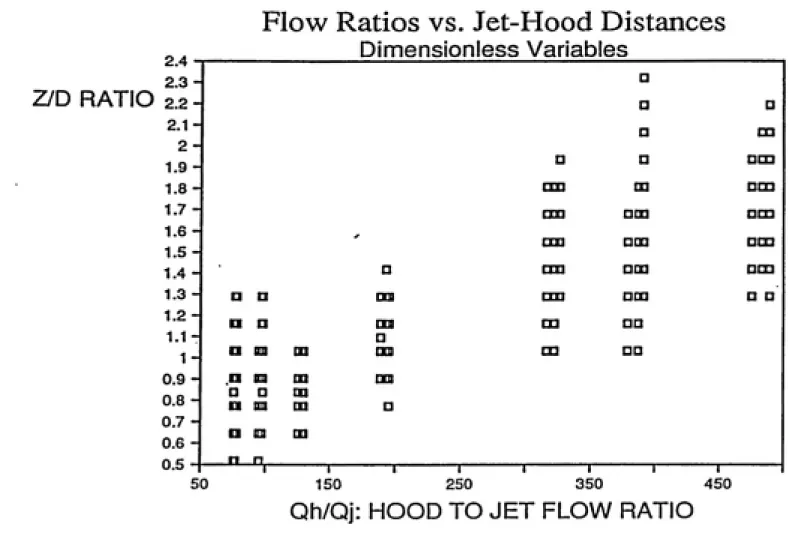
C. HOOD TO JET FLOW RATIOS VS. [Z/DJgQ:
PREDICTIONS AND CROSSDRAFT EFFECTS 7 3
D. THE ROLE OF e^, THE APPARENT
KINEMATIC (EDDY) VISCOSITY 80
VII. CONCLUSIONS AND RECOMMENDATIONS 82
VIII. REFERENCES 86
1. EXHAUST AIR SYSTEM
2. HOOD DESIGN TYPES
3. EQUAL VELOCITY CONTOURS
4. HOOD FLOW NOMOGRAM
5. POTENTIAL LINES AND STREAMLINES FOR AN FCH,
DISTURBED BY A CROSSDRAFT
6. IDEALIZED CONTAMINANT STREAMLINES
7. STREAMLINES IN A FREE CIRCULAR TURBULENT JET
8. VELOCITY PROFILES FOR AN AXISYMMETRIC JET
9. AXISYMMETRIC JET DIAGRAM
10. THE MIXING LENGTH CONCEPT
11. VELOCITY DISTRIBUTION IN A CIRCULAR TURBULENT JET 48
12. EXPERIMENTAL DESIGN 57
13. EXPERIMENTAL VS. PREDICTED [Z/DJgQ's 68
14. EXPERIMENTAL AND PREDICTED [Z/D]3q's vs. [Qh/Qj],
at 2 5 fpm CROSSDRAFT 7 4
15. EXPERIMENTAL AND PREDICTED [Z/DJ^q's vs. [Qh/Qj],
at no CROSSDRAFT 7 5
16. EXPERIMENTAL AND PREDICTED [Z/DJ^q's vs. [Qh/Qj],
at 5 fpm CROSSDRAFT 7 6
Paqe 4
6
9
13
22 24
37
38 40
Page
1. CAPTURE VELOCITIES 7
2. EMPIRICAL DESIGN DATA FOR NON-DIMENSIONAL
CENTERLINE VELOCITY GRADIENTS 16
3. SUMMARY OF INITIAL RESULTS 65
4. VALUES OF e^, AND OF CROSSDRAFT, REQUIRED TO
MATCH PREDICTED [Z/DJ^q WITH EXPERIMENTAL
A. RESEARCH COMPUTER PROGRAM
B. COMPUTER PREDICTIONS OF [Z/DJ^q's AT CR0SSDRAFT=25fpm
(3 EXAMPLES)
C. EXPERIMENTAL DATA, CALIBRATION THEREOF, AND
EFFICIENCY CALCULATIONS
D. DATA FOR REGRESSION OF LOGIT-TRANSFORMED EFFICIENCY
ON [Z/D]; CALCULATION OF w AND M
E. LOGIT CAPTURE EFFICIENCY REGRESSION ON [Z/D]
F. EXPERIMENTAL DATA: RESULTS SUMMARY
My sincere thanks are due to Dr. Michael R. Flynn
for his direction and enthusiasm for this research
project. His occasional suggestions were helpful, as was
the freedom he allowed me in pursing my intellectual
curiosity regarding adjunct issues. Appreciation is also
extended gratefully to my committee members Drs. Cass T.
Miller and David Leith. Dr. Leith provided the cyclone
and Venturi meter, without which this project would not
•
Industrial hygienists typically use a variety of
control measures to abate the danger to workers of inhaling
toxic materials. These may include engineering or
administrative controls, and possibly the use of personal
protective equipment. Because inhaled toxic materials may
give rise to a variety of deleterious health effects, it is
important to minimize such exposures.
Engineering controls are easily the more desirable of
protective measures because they ensure that the worker is
actually exposed to the toxin or otherwise hazardous
material as little as possible. Engineering controls in
general do not require active participation on the part of
the worker to be effective (controls are "designed in"), and
are therefore recommended over measures requiring
considerable training and, especially, supervision, such as
personal protective equipment or even administrative
rotation [1].
ͣ
Ventilation is a desirable and useful engineering
control. Dilution ventilation reduces the air concentration
of toxin in the entire work area by bringing in
uncontaminated air with which it is diluted. Dilution
ventilation is useful when the contaminant concentration or
•
exhaust ventilation is particularly necessary for close work
with concentrated toxic materials.
Local exhaust ventilation (LEV) is most usefully
designed so the contaminant does not have a chance to escape
in quantity into the room air. when LEV is properly
designed, other forms of protection, such as masks and/or
respirators may not be necessary. The basic elements of LEV
consist of a hood or hoods, ductwork, fan(s) and an air
cleaning system [2].
Hoods preferably are designed to be enclosures
encompassing the exhaust from the entire process. When this
is not possible, the hood may be placed to receive or
capture the bulk of the air flow from a process, and should
be placed as close to the process as possible. Receiving
hoods are placed so that the contaminant material will flow
into them. Grinding wheel hoods and canopies over hot
processes are receiving hoods. "Capture" hoods on the other
hand must be designed so the ventilation system creates a
strong enough flow field to entrain and capture the
contaminant. LEV hood design will be reviewed in the next
section.
The contaminant in air is removed through the ductwork
to the air cleaning device by the fan. By creating in the
ductwork a static pressure differential negative to the
atmosphere, the specifically-chosen fan moves a quantity of
particle size and density of the material expelled, the
toxicity thereof, and the cleaning efficiency required
[Figure 1].
The air cleaning device removes the contaminant from
the airstream brought to it by the ventilation system
described above. Air is usually exhausted to the outside
atmosphere through an exhaust stack once the particulates
and toxins have been largely removed. Under certain
circumstances, e.g., where atmospheric air would have to be
excessively heated or otherwise conditioned, some proportion
of exhaust air may be recirculated.
Designs of the LEV systems have remained fairly
stagnant since World War II, partially because the older
methods were seen as "adequate." Until the 1980s a relative
lack of theoretical work was available which would affect
system design concepts. The goal of such theoretical work
is not only to understand better the fundamentals, but is
also to provide workers with better protection for the
EXHAUST AIR SYSTEM
ENtB"^
DUCT
HOOD
FAN
CLEANER
A. CAPTURE VELOCITY CONCEPTS
Many different configurations of hood designs are
possible for control of the exhaust of every conceivable
industrial process. Nonetheless there are a few standard
designs that are used routinely, and which have been tested
widely. Slots, rectangular and round openings are the most
common; cabinets and booths are used to enclose whole
processes, and canopies are placed over evaporative
processes [Figure 2]. Traditionally, local exhaust
ventilation designs relied on a single unifying concept,
that of "capture velocity." The design equations developed
by Dalla Valle and Silverman in the 1930s all rely on this
design parameter, and it is the primary focus of designs
still promulgated by the ACGIH, in their Industrial
Ventilation Manual [3].
Velocity must be sufficient to entrain the contaminant
in the airflow toward the hood so it does not disperse or
settle out before being "captured" by the exhaust system.
Particular processes generate contaminants of different
HOOD raSIGN TYPES
HOOD TYPE
A=WL(sq.ft.)
H
^Cd
W
DESCRIPTION
SLOT
FLANGED SLOT
PLAIN OPENING
FLANGED OPENING
BOOTH
CANOPY
ASPECT RATIO W
0.2 OR LESS
0.2 OR LESS
0.2 OR GREATER AND ROUND
0.2 OR GREATER AND ROUND
TO SUIT WORK
TO SUIT WORK
SOURCE: REFERENCE 3
CAETURE VELOCITIES
Condition of Dispersion
of Contaminant Examples
Capture Velocity, fpm
Released with practically no
velocity Into quiet air.
Evaporation from tanks; degreaslng,
etc.
50-100
Released at low velocity Into
moderately sUll air.
Spray booths; Intermittent container
fining; low speed conveyor transfers;
welding; plating; piclUlng
100-200
Active generation Into zone of
rapid air motion
Spray painting in shailow booths;
barrel filling; conveyor loading;
crushers
200-500
Released at high Initlai velocity Into zone of very rapid air motion.
Grinding; abrasive blasting, tumbling
500-2000In each category above, a range of capture velocity Is shown. The proper choice of values depends on
several factors:
Lower End of Range Upper End of Range
1. Room air currents minimal or favorable to capture. 1. Disturbing room air currents.
2. Contaminants of low toxicity or of nuisance value 2. Contaminants of high toxicity,
only.3. Intermittent, low production. 3. High production, heavy use.
4. Large hood—large air mass In motion. 4. Small hood—local control only.
•
of a ventilation system typical for the process) taken from
or adapted from the ACGIH Manual.
For standard hood configurations such as round or
rectangular, flanged or unflanged hoods, Dalla Valle [4]
developed the original "rule-of-thumb" eguations. He
mathematically related several variables he found to be
characteristic of hood velocity values he measured at
various locations in front of LEV hoods. In general Dalla
Valle established the concept of the centerline velocity
gradient as a function of distance from the hood (X), volume
airflow (Q), and hood shape and flanging. He showed that
the surfaces of equal velocity into an exhaust hood were of
the same shape and relative position for all similarly
shaped hoods. While he mistakenly equated equal velocity
contours with equipotential surfaces, in alluding to
potential theory as a possible basis for description of
streamlines of airflow, he not only formed the basis for the
capture velocity concept, but also paved the way for the
theory which superceded it.
The use of a modified Pitot tube allowed Dalla Valle to
map the equal velocity contours of various exhaust hoods
[Figure 3]. A general equation was the result of his
studies:
f(Y) = m/(x"), (1)
lA, Cootocxj in ctnter-piane. perpendiculir Io lonj lide of opcnint.)
2 3 4*6
Dt«tonc« from Opening
IL, Coototin io ccDtcr-pUnc. pcrpcadieutar to ihott tide of opentnc.)
Fid. 3 Velocitt Contociu fob S-Ikcx dt 9-Inch OrrxiNO
X = the horizontal distance from the hood
along its centerline;
m = bA^,
where: b depends on the aspect ratio of a
rectangular hood, or = 0.0825 for
round hoods;
A = the hood face area;
k = a constant: 1.04; and
f(Y) = the point velocity at X, as fraction
of Y = the average face velocity.
Dalla Valle later simplified this model for round
hoods, or rectangular hoods with aspect ratio (AR =
width/length) greater than 0.2. This simplification has
been rearranged in the Ventilation Manual as:
V = Q/(10X2 + A), (2)
where: X < 3/2 D; . •
D = the hood diameter or side length;
V = the air velocity in feet per minute (fpm);
Q = volume flow in cubic feet per minute (cfm).
Dalle Valle believed that flanges reduce the volume
flow required by about 33% for the same required capture
velocity, so the simplified (ACGIH) equation for flanged
hoods became:
which Garrison [10] says is good for the region beyond about
.4D away from the hood face.
Several years after Dalla Valle's work Silverman
continued his investigations [5]. While he was unable to
improve upon Dalla Valle's simple equations for round hoods
and rectangular hoods of aspect ratios of >0.2, Silverman
was able to provide handy equations for slots (defined as
having AR < 0.2). His empirical solutions were:
for unflanged: V = 23.8 Q[(W+1)/W]/XL; and (4)
for flanged: V = 55.4 Q/XL, (5)
where: L = the length of the slot hood;
W = the width of the slot hood; and
X is defined as in the Dalla Valle equations.
These equations have been reduced and corrected in the
ACGIH Ventilation Manual to the
following:-for unflanged: V = Q/(3.7LX); and (5)
for flanged: V = Q/(2.6LX). (7)
A much more extensive investigation of the effect of
aspect ratio on the centerline velocity gradient was
conducted by Fletcher [6]. For fixed volume flows and hood
m
centerline increased as the AR decreased (became more slot¬
like) . Fletcher developed an equation for unflanged slot
hoods of AR's from 1:1 to 1:16 relating these variables, and
then constructed a convenient nomogram [Figure 4].
Fletcher's equation is:
V/V„ = 1/(0.93 + 8.58a^), (8)
where: a = [X/A'^] [W/L]"^; and
B = 0.2[X/A-^]"^/-^; and
Vq= hood face velocity; and
other variables are defined as before.
The effects of flanging on the centerline velocity were
studied subsequently by Fletcher [7]. Because flanges cut
down significantly on the volume flow necessary to produce a
given centerline velocity, they increase the efficiency and
decrease the cost of ventilation systems which use them [8].
He was able to demonstrate that the optimum flange width
equalled the square root of the hood opening area, and the
effect of the flange increases as the aspect ratio decreases
(becomes more slot-like). An adjacent surface [9] likewise
increases the centerline velocity of an exhaust hood by
cutting down the air volume from which flow is drawn into
the hood. Equal centerline velocities may be obtained in
TOO.
050.
^ 010 J
0-05 _
;
aoi_
0 005_
,0O5
[
005
_010
w L
_0-50
,100
FIGURE 4.
HOOD FLCW NOMX^RAM
(FLETCHER)
More recently. Garrison [10] has studied high
velocity-low volume (HVLV) systems and compared the results to the
work of Dalla Valle and followers. Generally, he found that
the ACGIH Ventilation Manual eguations were suitable, but
disagreed that flanging added 33% to centerline velocity
gradient values. He suggested that the actual increase is
probably between 10 to 30%. Silverman's equations cannot be
used very near the hood face, because as X approaches zero,
V at X becomes indeterminate; Garrison suggests that a limit
of accuracy of Silverman's equations (or their
simplifications in the ACGIH Manual) is reached when
centerline distance X to hood diameter or width ratios
X/D or X/W =0.4.
Garrison subsequently [11] conducted analyses of the
relationship of dimensional velocity ratios to
non-dimensional distance ratios for circular, rectangular and
slot hoods, for flanged and unflanged cases, and for various
aspect ratios. V, the centerline velocity at any given X
distance, may be related in a ratio to the hood face
velocity V^: Y = V/V^. Likewise, the centerline distance X
may be related in a ratio to hood diameter D, rectangular
hood width W, or slot hood length L: X^^ = X/D or X/W or
X/L. Then non-dimensional ratios Y and X^^^ may be related
to one another through empirically derived equations:
^("near") = ^(l^)^DW' ^^^ ^^^
•
where: a and b are empirical constants, which vary
depending on hood characteristics.
Later, Garrison expanded his explorations to include
other practice design concepts using various graphical
techniques for a number of "real-world" situations [12].
Obstacles and surfaces frequently block ideal airflow
streamlines, and methods such as sketching, conformal
mapping, and velocity vector addition may assist in the
evaluation of two-dimensional velocity gradients on the hood
centerline [Table 2].
A great deal of work has been done, summarized briefly
above, using capture velocity as the core theoretical
concept upon which practical design of exhaust hoods, and
analysis of exhaust hood flow, has been built. However,
there are significant deficiencies therein.
Recently, a number of investigators have criticized the
capture velocity concept. Heinson and Choi [13] have
provided a good summary of the problems associated with this
design method. It is as follows:
1) Contaminant concentration in the vicinity of
the source cannot be predicted;
2) The effect of changes in design (such as
system dimensions or volumetric flow) on the performance of
TABLE 2.
Empirical Design Data for Nondimensional Conterline Velocity Gradients
Y = a(bjXow Y
= a(Xow)'
Spaci Y Valu at Xow Nozz\a End Nozilo Profile Shape
OS Xow < 0.5 0.5 < Xow < 1.0 1.0 < Xow ^ Xow OS Shape
• b a b a b a b Xow 0.5 1.0
Plain no 0.06 .. .. 8 1.7
8 ͣ 1.7 1.5 26 3
Circular Flanged Flared
110 90
0.07
0.20 90 0.20
10 1.6 10
18 -1.6 -1.7 1.5 2.0 30 40 10 18
Rounded 98 0.50 145 0.23 -- -- 33
-2.2 2.5 69 33 Square Plain 107 0.09 10 1.7 10 -1.7 1.5 32 10
(WLR=1.0) Flanged 107 0.11 -- 12 1.6 12 ͣ1.6 1.5
36 12
Rectangular Plain 107 0.14
--18 1.2 18 -1.7 2.0 41 18
1WLR=0.50) Flanged 107 0.17 -- 21 1.1 21 -1.6 2.0
45 21
Rectangular Plain 107 0.18 .. 23 1.0 23
-1.5 2.5 46 23
(WLR=0.25) Flanged 107 0.22 -- 27
0.9 27 -1.4 3.0 50 27
Narrow slot Plain 107 0.19 ..
24 1.0 24 -1.2 3.5 48 24
(WLR=0.10) Flanged 107 0.22 -- 29
0.8 29 •1.1 4.0 50 29
3) Even though the performance of a particular
system is known, the effect of geometrically scaling it up
or down is unpredictable;
4) An engineer designing a system for a new
process (one for which an LEV design does not appear in
published literature) is left to design basically from
scratch with little knowledge of the effectiveness of the
resulting system;
5) The idea of providing a certain velocity to
capture contaminants is inconsistent with the laws of fluid
mechanics.
For example, Fletcher and Johnson [14] show that
traditional design methods are adequate for gases and
micron-sized particles released on the centerline of an LEV
hood at low velocities. But, especially if the direction of
release is away from the hood, if the release velocity is
higher than a certain low amount (0.21 m/sec in a certain
set of cases), higher "capture velocities" are required.
Moreover, as Ellenbecker et al. [16] point out, crossdrafts
and other air disturbances cannot be accounted for, energy
expenditure optimization is difficult, and there are
significant uncertainties in shaping the hood to distribute
velocity contours for efficient capture in three dimensions.
Only qualitative predictions of hood performance can be
•
Capture efficiency is a notion which may be
used to evaluate hood performance comprehensively. It is
useful because hood and system designs of all types may be
compared effectively to one another, and the effects of
changes in any design parameter may be evaluated along a
single scale.
Dalla Valle was guite aware of the inadequacies of the
theoretical approach in use at the time he was doing his
original work. He states [4]: "Without attempting to
minimize the importance of experience in engineering design,
it seems proper to point out that most of the past
experience in the design of local exhaust hoods has not been
associated with quantitative studies of the actual
efficiency of dust removal."
The first study using capture efficiency as the central
concept for the evaluation of hoods was conducted by Burgess
and Murrow [15]. Field conditions of contaminant generation
from machining operations were modeled in the laboratory,
and hood shape was demonstrated by the authors to be a
primary factor in the efficiency of contaminant control.
Once the central concept underlying hood design
changed, a new era in ventilation research began. However,
a careful definition of the new parameter was required.
Capture efficiency, r], is defined by Ellenbecker,
•
generated by a source that is captured by the LEV system
controlling it," or mathematically as:
ri= G'/G (11)
where: G'= the exhaust contaminant capture rate in grams
per second (g/s), and
G = the contaminant generation rate, g/s.
The capture efficiency is a function of at least five
variables: Q, the volume flow of the hood;
A, the hood face area;
X, the centerline distance of the hood to
the source;
V^, the crossdraft velocity; and
T, the temperature of the source.
When the temperature variable can be ignored, the
others may be analysed more easily. It is found by
application of the Buckingham it Theorem (see the relevant
discussion later in this section) that the capture
efficiency is related to a function of two (dimensionless)
ratios: the crossdraft velocity to hood face velocity; and
the centerline distance of source to hood divided by the
square root of the hood area:
The specific functional variable (K) and exponents
(a, b) defining the relationship are determined by
experiment.
The limiting conditions which apply are:
- 77 = 0 when X->-oo; (13)
r] = 0 when V^ = 0; (14)
?7 = 0 when V^ ^ 00; (15)
r] = 1 when X = 0; (16)
T] = 1 when V^ =: 0. - (17)
Actual measurement of capture efficiency in the
laboratory entails direct measurement of contaminant
concentrations in the duct of the exhaust hood. One must
assure good mixing within the hood's duct. Direct
measurement is made in the duct of the exhaust hood for the
contaminant concentration. The source is placed just within
the hood itself, to obtain the "100%" value. Then, the
source is placed at various distances X away from the hood.
The latter contaminant concentration values are compared at
every time interval measured with the 100% value, and the
ratio of the two is capture efficiency.
A subsequent paper by Flynn and Ellenbecker [17]
offered an analytically detailed approach to capture
efficiency, specifically to flanged circular exhaust hoods
(FCH). Their approach was based on the intuitive idea that
flow fields: 1) that generated by the hood; 2) the flow
field generated by the contaminant source; and 3) the flow
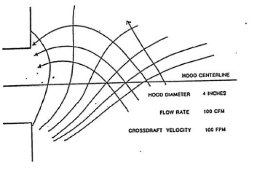
field due to perturbing crossdrafts [Figure 5]. It is the
interactions of these flow fields that ultimately determine
whether a contaminant enters the exhaust hood. Velocity
vector average values were determined for each field by
mathematical functions; in addition they accounted for some
degree of variability about these averages due to
turbulence.
In their model, Flynn and Ellenbecker calculated by
vector addition the path of streamlines of a contaminant
issuing in all directions from a point source, as they were
affected by the flow fields of the hood, and by a
crossdraft. They based their model on the modified
potential flow solution for airflow into flanged circular
hoods [18].
The cylindrical coordinate system is assumed in this
model such that the FCH centerline is the Z-axis. The
crossdraft is assumed to blow at velocity V^ perpendicular
to the Z-axis, from the 9 = 180° to the 8=0° half-planes.
The model assumes irrotational incompressible air flow, Q.
A series of point sources of isothermal nonbouyant gas
release at flow volume Qg, at some point (at distance Z)
from the FCH. Flynn and Ellenbecker developed a computer
model for the IBM XT personal computer [17] which maps the
HOOD DIAMETER * INCHES
FLOW RATE 100 CFM
CROSSDRAFT VELOCITY 100 FPM
Figure 5 — Theoretical potential lines and streamlines for a
flanged circular hood operating in the presence of a crossdraft
perpendicular to the hood centerline.
K
exist in the plane of the Z axis, and shows whether or not,
when under the combined influence of the hood flow and
crossdraft flow, they enter the FCH [Figure 6].
Previously developed similar models include
Fialkovskaya•s simplified point-sink model in which he
described eguations for the streamline which would just
enter a hood in the presence of a cross-draft [19], and
Strauss' modified n-sinks model allowing iterative
processing [20]. Empirical studies have validated Flynn and
Ellenbecker's "Final Model" [21]; their work recently has
been extended to mathematical analysis and quantitative
evaluation of potential flow modeling for hoods of other
configurations [22].
To calculate capture efficiencies in such systems, one
must apply the Buckingham it theorem. The ir stands for the
Product of variables. Each tt is a dimensionless group of
variables formed by application of the theorem. The theorem
assures that for a process depending on n dimensional
variables, then a reduction to k dimensionless variables is
possible, where n-k = j, where j is the maximum number of
variables which do not form a it among themselves. The
reduction number j is always less than or equal to the
number of dimensions (time, length, mass, temperature), m,
in the n descriptive variables. The choice of the n
dimensional variables is critical; if one is inadvertently
T>= 4 IN.
Q= 104 CFM
U= 114 FPM
\
FIGURE 6.
IDEALIZED CONTAMINAM: STREAMLINES
In the capture efficiency analysis, each of the
following variables:
D = diameter of the hood;
Z = distance to the point of origin;
Q = the volume flow of the hood in cfm; and
V^= the velocity of the crossdraft,
must be considered. Application of the Buckingham n theorem
suggests that one dimensionless group will be [Z/D], and the
second will be [V^/V^], where the hood face velocity is
extracted from the hood flow variable. A third
dimensionless group, [Qg/Q] will appear when the contaminant
source flow [Qg] is considered with the other variables.
However, the functional relationship between the tt ' s
cannot be specified explicitly without experiment. The
[Z/D] is the ratio of the hood-source distance to the
diameter of the hood. It will have a profound effect on
capture efficiency. Near the hood, most of the source of
flow will be captured by the hood's flow field; if the
source is far away the hood's field is weak. The second
group [Vj/V^] is the ratio of face velocity to that of the
crossdraft. The weaker the crossdraft, the less distorted
are the effects of the hood and its flow field. Similarly
with [Qg/Q], the hood flow field will have predominance over
a contaminant source with a low flow rate.
The use of plotted streamlines from the source to the
hood is important; each streamline either does or does not
streamlines enter the hood defines the capture efficiency
for that particular set of conditions [Figure 6].
Alternatively, when a single streamline is calculated
from a point source, it may be seen statistically as the
first moment of distribution of the flow from that source;
turbulence and dispersion are assumed to be equally
distributed around such a streamline. When such a
streamline hits the edge of the hood, half the flow is
assumed captured and half is not. The distance Z from the
hood to the contaminant source then forms a dimensionless
ratio with the hood diameter D; and at the point of probable
50% capture, is designated [Z/DJ^q, the "critical distance."
It is assumed that turbulence is primarily accounted for by
the [Vj/V^] ratio; it is used as a predictor for the effects
of turbulent diffusion on contaminant dispersion around the
streamline. The computer model can be used iteratively to
obtain the [Z/DJ^q for any given combination of other
variables. Then one determines the regression between the n
III. BACKGROUND TO THE COMPUTER MODEL
A. ELEMENTS OF POTENTIAL THEORY
Since Flynn and Ellenbecker's model [17, 21] is
based on the potential flow solution [18], they are assuming
that the airflow into the exhaust hood is incompressible and
irrotational. Moreover, in potential flow, frictional
forces are negligible, so that inviscid flow is assumed.
Laplace's equation:
V^ $ = 0 (18)
is used to describe such a flow field.
Laplace's equation is derived from the continuity
equation:
[d[/dt] + v'(r V) = 0 ' (19)
where: f = the fluid density;
t = the elapsed time;
^= del, the gradient operator; and
V = the velocity vector.
The continuity equation is the summary of conservation
of mass requirements in fluid mechanics. Continuity is said
to exist wherever the volume flow, Q, equals the area of any
hypothetical velocity contour surface times the velocity
Incompressibility of a fluid means that density changes
are negligible, so the first term drops out, and the
continuity equation becomes:
V'v =0, / (20)
and it is said that the "divergence" of the velocity field
is zero. "Divergence" is a measure comparing flow into and
out of a defined differentially small control volume in
space. When it is zero, all fluid flowing into such a
volume leaves at the same rate. The velocity field then is
neither converging (volume shrinking with increasing
density) nor diverging (getting larger with decreasing
density). About 330 ft/sec is the upper velocity limit for
incompressible flow of standard air.
The gradient operator, ^, can be written out as:
V( ) = [9( )/dx]r+ [d{ )/9y]T+ [d{ )/5z]k (21)
in a three dimensional (x, y, z) coordinate system. The
gradient operator converts a scalar to a vector function,
and when solved gives the direction and maximum rate of
increase of the function.
An irrotational fluid flow has no vorticity or "curl."
In the mathematical description of an irrotational fluid,
the cross-product of the gradient operator and the velocity
vector function must always equal zero:
because the angular momentum of an irrotational flow is
zero.
From this it follows directly (partly by definition)
that the velocity vector function is the gradient of a
"potential" function:
V = V* (23)
where $ is the (scalar) potential function. Substituting
equation (23) into equation (20) yields Laplace's equation
(18) .
The "potential" function, $, is defined for every point
in space (x, y, z) as "the sum of the potential of the
extraneous impulsive forces by which the actual motion at
any instant could be produced instantaneously from
rest" [27]. The potential function may be analysed as the
product of time and force, divided by area and density:
tF/Af; simplified, the units are usually cm^/sec.
Viscous forces are negligible in potential flow.
Inviscid flow occurs where no solid surfaces exist over
which boundary layers would form. It is assumed in the
strict potential flow model for FCH's that all hood flow is
potential flow. This simplifying assumption yields results
which are inaccurate only at points close to the hood face.
Using the assumptions of potential flow, and within
to define the velocity flow field. Boundary conditions are
B. POTENTIAL FLOW SOLUTIONS FOR FLANGED CIRCULAR HOODS
The potential flow solution is described in detail
in Flynn and Ellenbecker's original papers [18, 21]. The
potential flow model for the FCH was developed because it is
amenable to practical application, in contrast to the more
accurate, but difficult, constant velocity analytic
solutions of Lamb [27] and Drkal [28].
In contrast to centerline velocity gradient studies,
potential flow solutions describe the velocity field of
airflow into the hood in three dimensions. This is
particularly useful and important where sources are not on
the centerline, where there is significant dispersion, where
the direction of contaminant generation is not directly
toward the hood face, or where there is a crossdraft.
Boundary conditions and simplifying assumptions for the
potential flow model for the FCH are:
1) an infinite flange;
ͣ
2) no flow through the flange: 3$/3z = 0, for
the conditions z = 0, r > a, where a = the hood radius;
3) constant potential, $, at the hood face; and
4) f ^ 0, as X -^ 00.
The strict potential flow solution however, is not
entirely adequate. The assumptions of inviscid,
irrotational flow begin to break down in the region near the
importance of shear stress due to turbulence of the boundary
layer, and vena contracta formation. Real centerline
velocities at the hood face are about twice the predicted
value. Additionally, the strict potential flow solution
predicts infinite velocity along the edge of the hood.
However, turbulence there considerably reduces actual air
velocity.
To address these anomalies in the theory, Flynn and
Ellenbecker noted that Dalla Valle's equal velocity contours
are elliptical. They make the assumption that the velocity
vector field is uniform everywhere along each confocal
ellipsoid equipotential surface provided by the theory. (In
reality, the velocity field is the gradient of the
potential.) For their modified potential flow solutions, a
set of conditions, similar to the boundary conditions for
the strict solution, apply, with the exception that in
addition the hood face velocity is constant. The derived
expression for velocity at every point in the field is then
reasonably consistent with experiment. Additionally,
because Laplace's equation is linear, other potential flows
may be added vectorially at any given point. Thus,
crossdraft effects and source vectors can be added to affect
the velocity vector field of the hood.
In the validation of their solution [21], Flynn and
Ellenbecker considered three versions of their model. The
first was the strict potential flow solution. The second
between an "inconsistent" model and one which contains a
singularity. While "an inconsistent model is one that is
not exact mathematically, a singularity refers to a region
where unrealistic fluid behavior occurs." Thus while Model
1 is a consistent model, it is also a singular one. Model
2, however, is inconsistent due to the "inexact"
approximation made to obtain it. The modified velocity
field equation cannot be integrated to give the true Q; for
example, the theoretical (Model 2) average face velocity is
87% of the true value.
Flynn and Ellenbecker's Final Model employed a radial
correction factor C^,, a strong function of the eccentricity,
where: C^. = 2.6 e-'-^ + 0.853. The eccentricity, e, is the
ratio of the hood diameter to the sum of the distances from
the edges of the hood opening to the point in question:
2 a
e = --- . (24)
(ri + r2)
Here, r-,_ = y[ z2+(a^ + r^) ] , and r2 = /[ z'^+(a^^-r^) ] . The
radial correction was necessary because the radial velocity
as measured increased more rapidly than predicted as the
eccentricity approached 1 (i.e. near the hood face).
Additionally, the theoretical axial velocity
calculations were also adjusted, by a factor of 0.9, based
on the graphical results of the validation experiments.
These empirical corrections were an attempt to overcome the
The modified potential flow solution calculates the
velocity at any point in the hood coordinate system
(R, 6', Z) as:
2 TT a^ y(3-2e'=^7
Vt2 = ---Z--
ͣ
. (25)
The Final Model component velocity vectors are:
Vp = -Cj, Vrp2 (sin P) ; and (26)
V^ = -0.9 V^2 (^°^ ^)' (27)
where: /? = tan """ (Vj^i/Vzi) , and (28)
where Vj^-^^ and V^^-^ ^^^ calculated as defined in both papers
[18, 21] .
The Final Model was incorporated into an interactive
BASIC program, which required the input of three variables:
D = the hood diameter in inches;
Q = the hood flow in cubic feet per minute, cfm;
V^= the crossdraft velocity, feet per minute, fpm.
The output for one of the possible combinations of
located in those regions from which the streamlines are
drawn into the hood. The program just described forms the
basis of both the experiments and program modifications for
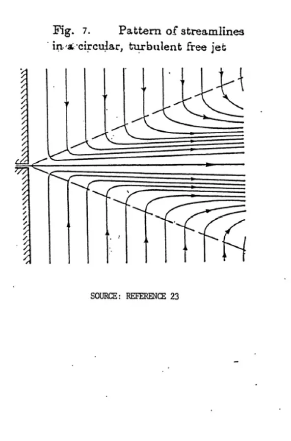
C. CIRCULAR JET FLOW AND THE SCHLICHTING EQUATIONS
An ideal circular jet of fluid, flowing into a
still medium, maintains constant static pressure throughout
itself. However, the flow, Q, the area. A, and the jet
width, b, are not at all constant; they are continually
increasing with the entrainment of the surrounding air
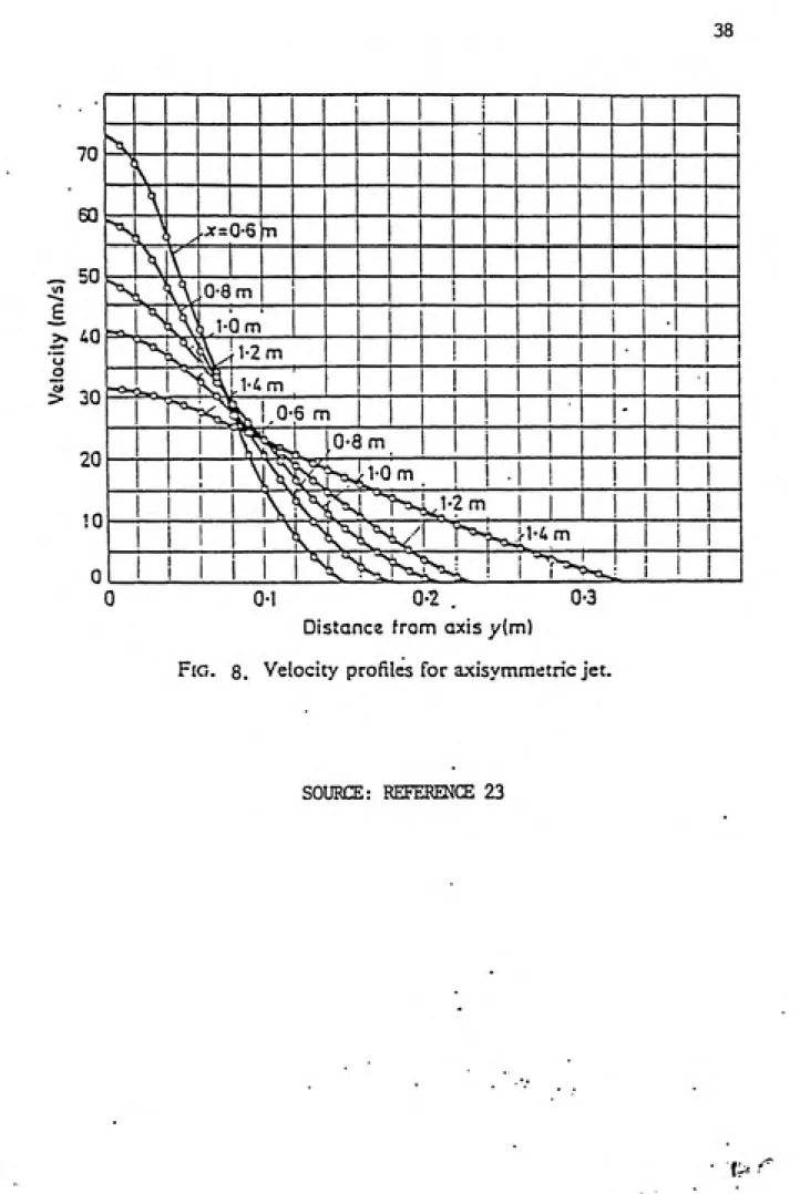
[Figure 7]. Its energy losses are likewise proportional to
jet length, almost entirely in kinetic energy (i.e. in
velocity) [Figure 8]. The momenta of external forces on a
jet entering still air sum to zero, so the momentum of the
mass flow of air (kinematic momentum) throughout such a jet
remains constant [19].
The kinematic momentum, K, can be calculated for a jet
of known flow. Since, in cylindrical coordinates
K = 27r
00
V^^ r dr, (29;
where: V^ = velocity in the axial direction of the jet, and
r = the radius of the jet flow at z; and
since at z = 0, V^ is not a function of r, then simple
integration will yield:
Fig. 7. Pattern of Streamlines
in- * circular, turbulent free jet
i
1—I
70
\,
i
V
60
\
N
\
L^
.;c=0-6
T>^ 50
\
\
H '
\W
0-8 m
>, 40
Kirt-w^
3 1-Qm'
j 1
1
ͣ'^Nv^"^^kJv2 m
i J
o
^ 30
-c^,_^l^lUm',
'
'i 1 1
r^>CS;hi.Q-6m
-20
l^^
.0-8 m
11
1
1 YW^lh^J"'^ ^ 1 !
ͣ
i
10
1 ! !
1 KX?^"N4j-2m
!
1 i 1
1 i !
1 i \XN^<'^
1 TH^'^'^ .
i > ) 1
III!
0
i M i 1 I^VKKl ! i"f-i^
1 i
i i I
i 1
0-1 0-2 . 0-3
Distance from axis y(m)
Fig. 8. Velocity profiles for axisymraetric jet.
70
60
_ 50
u
o
I 30
20
1
!
—I 1
>^.
'
i
\
\
psJ
\.^
.;f=0-6
Tl
\
k
k,^
\^
0-8 m
i
1
ro-.
UVi
iJ-Om
•
rv^U'-2m
!
i i
po<
>«i^'^^O.l-^rn \
n r" 1
"^^T
"""S-S^ \0-5 m
-"^"fti
.0-8 m
1
1
1 m?>^l-On,, I i .
i
1 Kw^-t-^j-z- 1 1
!
i ! '
1 1 \X":i^^
[^f^^f^l-im
1 1 1 1 i 1 lXV>CS>vi ! 1-^^
' ' 1 '
ͣ
Q-l 0-2 . 0-3
Distance from axis y(m)
Fig. 8. Velocity profiles for axisymmetnc jet.
since flow equals the product of area and velocity. For any
given jet flow, Q, and starting velocity, V, we can thus
calculate K.
The spread of a circular jet can be described [23] as
beginning at a single point ("pole" or "virtual point")
[Figure 9]. Experimentally, it has been discovered that for
a cylindrical jet the virtual point is located 1.86 times
the jet opening diameter, inside its opening [19]. It is
there that the flow calculations must begin. See the
program, located in the Appendix.
Lines drawn from the virtual point through the orifice
edges then extend outward such that they form the boundary
of the mixing zone. With increasing distance from the
origin, the material in the jet core becomes diffused by
mixture with the surrounding air. In the core (in the
"initial section"), the velocity profile remains square, and
the temperature and concentration remain constant. The core
tapers. In the "main section," the velocity profile widens
and flattens. Throughout, the velocity profiles are
symmetric, and similar.
Turbulent jet flow is characterized by a cross-transfer
of vortices, and as these move beyond the limits of the jet,
impart their momentum to surrounding layers of air.
Main section
Initial section
C
V
zmx
i.Q^d—^
Fig. 9. Axisymmetric jet.
entire periphery it "meets itself" on the axis of the jet
[Figure 9]. In the main section of the jet, the entire flow
is turbulent.
In a circular jet, the amount of turbulent shear stress
associated with the boundary layer can be analyzed by
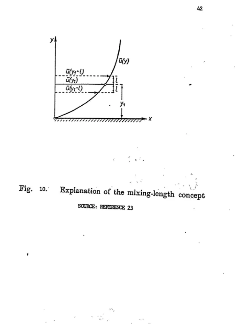
Prandtl's modified mixing length theory. To visualize a
physical interpretation of "mixing length" one must use a
simple model of turbulent flow of a jet along a wall [Figure
10]. This is the simplest case of parallel flow, in which
velocity is assumed to vary only from streamline to
streamline. As the flow progresses and turbulent mixing
zones move longitudinally, they also may move transversely,
while retaining their momentum.
Prandtl's mixing length, 1, is defined as "that
(transverse) distance which must be covered by an
agglomeration of fluid particles, travelling with its
original velocity, in order to make the difference between
its velocity and the velocity in the new lamina equal to the
mean transverse fluctuation in turbulent flow" [23].
The overall variations in the velocity contours of the
jet are controlled by this transverse movement of turbulence
eddies. The thickness and rate of motion of the mixing
layers is a critical determinant in the calculation of the
magnitude and direction of the velocity vectors at any given
point in the jet.
y+
Fig. 10. Explanation of the mixing-length concept
extent of lateral movement. Prandtl's mixing length
hypothesis combines the equation describing this relation,
with the equation for the shearing stress of the turbulent
flow, and obtains an equation hypothetically describing the
turbulent shear stress, t^, in terms of:
f = the density of the flowing medium;
1 = the thickness of the laminae defining lateral
movement; and
dii/dy = the rate of change of mean velocity between
laminae:
T^ = i^ 1^ |du/dy| du/dy, (31)
where the absolute value operator is to ensure the proper
sign of the result. Equation 31 is the formal definition of
Prandtl's mixing length hypothesis.
Turbulent flow contains both time-average (mean)
motions, and fluctuating (eddying) motions, in all three
directions. Over a sufficient length of time, the
time-average of all the eddying motions sum to zero. However,
these fluctuations influence the mean motion such that the
mean motion exhibits an apparent increase in resistance to
deformation: the apparent (or virtual) viscosity, or "eddy
viscosity." A mixing coefficient has been introduced in the
fluid dynamics literature, A^, for this Reynolds stress of
turbulent flow. It is analogous to the Stokes coefficient
of viscosity for laminar flow, /i-|_, and it likewise relates
r^ = A^ du/dy. It is not, however, a fluid property like
the coefficient of viscosity, and its value depends on the
mean fluid velocity. The apparent kinematic viscosity, e^,
is likewise analogous to the derivation of kinematic
viscosity of laminar flow, v-|_, and is defined as the mixing
coefficient divided by the fluid density.
In order to cure a theoretical defect in the
calculation of the apparent kinematic viscosity, e^, based
on Equation 31 and its assumptions, Prandtl modified its
derivation. The modification is valid only in free
turbulent flow, and is derived from extensive experimental
data. The original hypothesis had assumed that the volumes
of fluid moving transversely during turbulent mixing had
diameters very small compared to the transverse dimensions
of the movement. The modified hypothesis [23] assumes the
diameters of the transversely-moving volumes of fluid are of
the same order of magnitude as that of the mixing zone,
"The virtual kinematic (eddy) viscosity, e^, is now formed
by multiplying the maximum difference in the time-mean flow
velocity with a length which is assumed to be proportional
to the width, b, of the mixing zone":
' ' ;
ͣ
^T = ^1 ^ (^max-*^min) ' (^2)
where x-[_ is a dimensionless experimentally-derived constant;
with this treatment, e^ remains constant throughout the
proportionality of length and width of the jet, and the
simple inverse proportionality thereof to velocity, the
virtual kinematic viscosity of turbulent flow, e^, becomes a
constant, e^, over the entire length of the jet.
As a result, the velocity distribution differential
equations become formally similar to those of laminar jets;
only the term therein for kinematic viscosity of laminar
flow (v-j_) needs to be replaced by that for the virtual
kinematic viscosity (e^) of turbulent flow.
To calculate the vector equations, one must know how to
calculate e . According to measurements by Reichardt
[referenced in 23], the half-width, h^, of a circular
turbulent jet at the point where V^ - one-half the maximum
centerline velocity, is given by:
- bi = 0.0848 z, (33)
where: z = the distance from the nozzle.
Reichardt's measurements also yielded an equation:
bx, = (5.27 z
€
q)/ yK (34)
that can be used in conjunction with the previous one, such
that for any given value of z, and with K determined as
previously discussed, e^, the virtual or apparent kinematic
In summary, given a few fairly reasonable simplifying
assumptions, it is possible to calculate two critical
characteristics of the flow of a circular turbulent jet.
The kinematic momentum, K, and the eddy viscosity, e^, are
calculated by knowing: 1) the flow, Q, and initial
velocity, V; and 2) the axial distance, z, of any
particular point in the jet.
As alluded to earlier, there is formal similarity of
the equations for the velocity vectors of turbulent flow
with those of laminar flow. For a turbulent jet, V^ is the
magnitude of the velocity vector in the direction of the jet
axis (z):
3K
V^ = --- , and (35)
8 TT e^ z [l+.25772]2
Vj_ is the magnitude of the velocity vector in the radial
direction (r):
J 3K [77-.25r]-^]
V^ = ---^— , (36;
4 yF z [l+.25r]^]'^
where in either case:
r^^
A JT e^ z
(37)
Reichardt evaluated this model by comparing the
with the distribution of experimentally-determined velocity
values, for three different axial distances [Figure 11]. The
axes of Figure 11 are in dimensionless ratios. There is
impressive correspondence between the experimental findings
X "ZOcm
" '26 an
'tScm
Fig. 11. Velocity distribution in a circular, turbulent jet. Meaaurementa due to Reichardt
IV. PURPOSE AND OBJECTIVES
The purpose of this work is to validate a computer
model that predicts the streamline that a jet of gaseous
contaminant will follow in the flow field of a flanged
circular hood. These studies will assist in developing
reliable estimates of breathing zone concentrations of
gaseous or other jets of workplace contaminants.
The objectives of this research are:
1. To write a new interactive computer program to
describe the flow of a circular turbulent contaminant jet
within the flow field of a flanged circular exhaust hood.
This is accomplished by combining a modified BASIC
computer program from Flynn and Ellenbecker [21], for the
validated potential flow solution for airflow into a
flanged circular hood, with the appropriate expressions
for the velocity vectors of the flow of a circular jet;
2. To run the program for a matrix of hood and jet
flows, and distance values of the jet from the hood face,
to create predictions of the specific hood centerline
locations of the jet, [Z/DJ^q, at which half of the jet
flow would be captured by the exhaust hood; and
3. To perform replicate laboratory experiments for
each combination of hood and jet flows and distances, to
determine actual [Z/D]5q values for each, and to compare
A basic premise of potential theory is that of a
free field, in which there is unbounded, unobstructed
flow. Inviscid flow may be assumed, and this assumption
allows the neglect of friction. The use of strict
potential theory in the description of hood flow yields
an analysis in which the gradient of potential (the
magnitude of velocity vectors) varies strongly along the
confocal ellipsoids of equal potential. For the modified
potential flow solution, a simplifying assumption is made
[18], equivalent to Dalle Valle's original error. It is
that the equal velocity contours found in experimental
work are equivalent to the equipotential confocal
ellipsoidal surfaces described in potential flow field
theory. This simplification, with appropriate correction
factors [21], yields a quite accurate descriptive model
of an unobstructed FCH flow field.
When plumes of jet contaminant are introduced, an
appropriate jet-flow theory must be used. The Prandtl
mixing-length hypothesis for turbulent jet flow, which
assumes a constant virtual kinematic viscosity, and
yields a constant kinematic momentum, seems to be
applicable; viscosity is an important consideration in
its derivation. The Schlichting equations calculate the
velocity vectors of any given point in the flow field of
the jet. It is assumed that each of these vector
quantities calculated for each corresponding point along
streamlines of the flow field of the hood. Vector
additions are made iteratively at desired increments, to
obtain the entire combined streamline.
This model of combined flow is validated
experimentally. Computer predictions are made of the
specific locations along the hood centerline of the jet,
such that a 50% capture efficiency is achieved by the
hood. This is necessary to determine if the velocity
vectors of the two parts of this model, one (for the hood
flow) which ignores viscosity, and the other (for the
jet) which assumes its significance, can be added
together to predict Jetstream trajectory while in the
flow field of the hood. If so, then the entire field of
points of actual jet location can be mapped such that the
capture efficiency of the hood is at least 50%.
V. METHODS
A. COMPUTER MODEL
The computer model is composed of the union of two
parts, with accompanying reminders, explanatory notes, and
instructions for graphic display and printouts. The two
parts of the computer model are: 1) those that describe and
calculate the flow field of the flanged circular exhaust
hood; and 2) those that describe and calculate the flow of a
free turbulent gas jet. Each of these parts of the overall
program calculates the vector magnitude and direction of
velocity in its own cylindrical coordinate system. These are
denoted as (r, 9, z) for the jet, and (R, 9', Z) for the
hood.
The jet is arranged in relation to the hood such that
its tip is in front of the hood on the hood centerline, and
the jet centerline (z) axis is perpendicular to the
centerline (Z) axis of the hood. The "base plane," in which
all calculations are done, is the plane of the two (hood and
jet) centerlines.
Vector transformations are contingent upon the original
orientation of the jet to the hood. The hood's R
directional axis for calculation purposes was in the
half-plane of the base half-plane in the direction of original jet
flow. Additionally, only the r-vector of the jet in the
the specific arrangement of jet to hood axes chosen, there
was no 0 component (rotation out of the base plane) to be
considered for either jet or hood. In the base plane,
r-and z-direction vector magnitudes of the jet were
transformed into the coordinate system of the hood, prior to
the calculation of their combined magnitude. They were also
calculated to account for the distance of the virtual point,
within the tip of the jet tube, from the tip of the jet
nozzle.
In order to account for the effects of the flange of
the hood on the flow of the jet, use is made in the computer
program of an image jet located "behind" the flange, the
vector calculations for which are assumed to be equal and
opposite to its real counterpart. It is necessary for the
proper calculation of the velocity vectors of jet flow.
Any given velocity vector for the real jet equals the scalar
sum of the corresponding velocity vectors of both the real
and imaginary jets. Thus, when combined, jet velocity
vectors will be calculated to yield streamlines which follow
a path which "sees" the barrier the flange presents.
The velocity vectors of the hood and jet flows are
iteratively calculated and added (once transformed to the
same coordinate system) for the entire length of the
centerline flow of the jet within the flow field of the
hood. The program directs the display of the jet's
calculated centerline in relation to a cross section of the
run, it may be used to calculate the jet trajectory for any
given hood flow (Q^) ^ J^t flow (Q-;), jet-to-hood distance
(z), and crossdraft velocity (V^) parallel to the axis of
the jet.
The program can be run, using the given assumptions,
with the jet pointing along any quadrant line. The jet
could be placed pointing away from the hood ---0° to the
hood Z axis--- or toward the hood (180°) along its axis. In
contrast, the arrangement tested for the experiments
reported in this thesis is placement of the jet axis
perpendicular to the hood axis. Note that, without a
crossdraft, a 270° placement is equivalent to 90°.
The program displays, for each run, the following
variables: