Sharif University of Technology
Scientia IranicaTransactions E: Industrial Engineering http://scientiairanica.sharif.edu
Resilient supplier selection and order allocation under
uncertainty
N. Sahebjamnia
Department of Industrial Engineering, University of Science and Technology of Mazandaran, Behshahr, P.O. Box 4851878195, Mazandaran, Iran.
Received 21 November 2017; received in revised form 27 May 2018; accepted 11 August 2018
KEYWORDS Resilient supply chain; Supplier selection; Order allocation; Mathematical modeling; Uncertainty.
Abstract.Increasing the number of disasters around the world decreases the performance of supply chain. The decision makers should design resilient supply chain networks that can encounter disruptions. This paper develops an integrated resilient model for supplier selection and order allocation. Resilience measures including quality, delivery, technology, continuity, and environmental competences were explored for determining the Resilience Weight (RW) of suppliers. Fuzzy Decision Making Trial and Evaluation Laboratory (DEMATEL) and Analytic Network Process (ANP) methods were applied to nding the overall performance of each supplier. Then, the developed mathematical model maximized the overall performance of suppliers while minimizing total cost of network. The proposed mathematical model helps the decision makers to select supplier and allocate the optimum order quantities by considering shortage. Since the disruptive incidents are inevitable events in real-world problems, the impact of disruptions on suppliers, manufacturers, and retailers has been considered in the proposed model. Inherent uncertainties of parameters were taken into account to increase the compatibility of the approach with realistic environments. To tackle the uncertainty and multi-objectiveness of the proposed model, interval method and TH aggregation function were adapted. The proposed model was validated through its application to a real case study of a furniture company. Results demonstrated usefulness and applicability of the proposed model.
© 2020 Sharif University of Technology. All rights reserved.
1. Introduction
Rapid development toward globalization, competitive marketplace, remarkable advances in technology, and high expectations of costumers have convinced com-panies to reduce costs and increase their competitive advantages [1]. A supply chain encompasses suppliers, manufacturers, distributers, retailers, and costumers, beginning with purchasing raw materials and ending *. Tel.:+98 11 34552000
E-mail address: n.sahebjamnia@mazust.ac.ir doi: 10.24200/sci.2018.5547.1337
with consumption of the nal product by the cus-tomer [2]. Due to the presence of various actors, decision making issues in the supply chain are more complex than those in other areas. Decisions in supply chain management have been classied into three cat-egories at strategic, tactical, and operational levels [3]. The main decisions in strategic level are partnership selection and supply chain network design as they have the most extensive eects on the performance of the network [4]. Procurement [5], production [6], distribu-tion planning [7], and order allocadistribu-tion [8] challenges are the most important issues at the tactical level. Finally, at operational level, decisions such as production and transportation scheduling are considered [9]. Unstable
situations and unexpected incidents among supply chain actors force decision makers to recognize the optimal decision at any level and in any situation. Therefore, they need to update the supply side by choosing suppliers and allocating orders jointly and rapidly [8].
Researches have demonstrated that supplier selec-tion (at strategic decision level) and order allocaselec-tion (at tactical decision level) decisions have a signicant in-uence on the performance of the supply chain [10,11]. This inuence becomes more prominent when several supply chains have been disrupted by disasters or crises. In such situations, generally, the actors lose their resources and, consequently, they cannot deliver their products to the next level in the supply chain network [12]. To tackle this issue, decision makers have to consider the resilience features for choosing suppliers and determining order quantity. Despite the growing concerns about disruption in supply chain network design problems, few scholars have considered the resilience features to solve SS&OA problem [13].
This paper develops an integrated resilient model of SS&OA under uncertainty. At the rst stage, re-silience measures are explored for choosing appropriate suppliers according to resilience features. Then, the weight of each supplier is determined by applying two well-known multi-criteria decision making meth-ods, namely fuzzy DEMATEL and fuzzy ANP. The Resilience Weight (RW) of each supplier is used to develop a new fuzzy multi-objective mixed-integer lin-ear programming model. The proposed mathematical model helps the decision makers to select supplier and determine order size as well as shortage through minimizing total cost and maximizing resilience of the supply chain. Since the disruptive incidents are inevitable events in real-world problems, the impact of disruptions on suppliers, manufacturers, and retailers is considered in the proposed model. In addition, inherent uncertainty of parameters is taken into ac-count to increase the compatibility of the approach with realistic environments. To tackle the uncertainty and multi-objectiveness of the proposed model, interval method and Torabi-Hassini (TH) aggregation function are adopted. The proposed model will be validated through its application to a real case study of a furniture company. The main contributions of the paper can be outlined as follows:
Developing an integrated model for SS&OA by considering shortage;
Considering the impacts of the disruptions on the actors of the supply chain;
Evaluating suppliers with the resilience measures to increase the capability of supply chain against disasters or crises;
Validation of the proposed methodology through the case study of a furniture company.
2. Literature review
In today's competitive market, an organization has to optimize its business process through collaborating with other actors of the supply chain. Each actor in a supply chain (i.e., supplier, manufacturer, distributer, and retailer) aims to increase the total performance of the network [14]. One of the most important decisions, which impacts the performance of all actors, is SS&OA [15]. In recent years, this problem has been considered by many scholars as an integrated decision (at strategic and tactical decision levels) in the supply chain to achieve positional competitive advantage.
Several approaches to the SS&OA problem have been developed. Since decisions are made based on conicting criteria, these approaches can be categorized into two main groups of analytical framework (or attribute decision making methods) and multi-objective mathematical models [16]. Many scholars have utilized both categories, simultaneously, for se-lecting supplier and allocating order [17,18]. For example, Hammami et al. [19] considered a global supplier selection problem in which price discounts and uncertain uctuations of currency exchange rates played a crucial part. They formulated the problem as a mixed-integer scenario based stochastic model in two stages. At the rst stage, the model sought to select appropriate suppliers and total order quantity, while at the second stage, the model optimized order size in dierent periods. Goren [20] proposed a hybrid decision framework for selecting supplier and allocating order quantity regarding sustainability factors. He applied fuzzy DEMATEL and Taguchi loss functions to calculating sustainability weight of each supplier. The results demonstrated the applicability and useful-ness of such hybrid method [20]. Indeed, this paper developed a two-steps decision framework for deter-mining the RWs of the suppliers (utilizing analytical framework) and then, selecting supplier and allocating order quantity to them (developing a multi-objective mathematical model). Chai et al. [21] reviewed the applications of dierent decision making techniques to the SS&OA problem. They concluded that Multi-Attribute Decision Making (MADM) methods such as AHP and ANP were the most frequently used ones due to their eectiveness in ranking. Moreover, fuzzy sets are capable approaches to dealing with the uncertainty in SS&OA problem [22]. Keshavarz Ghorabaee, et al. [23] reviewed the application of the fuzzy MADM methods to SS&OA in uncertain environment. The review included 11 well-known MADM methods ap-plied to 339 relevant problems. It emphasized the insucient attention to fuzzy DEMATEL and ANP
hybrid method in the previous studies for solving SS&OA problem, while, although the fuzzy DEMATEL and AHP hybrid method had been used more than fuzzy DEMATEL and ANP, the ANP method could include the whole interrelationships between selection factors [23]. Accordingly, they intended to apply the DEMATEL and ANP hybrid method to calculating the RW of the supplier.
Rezaei and Davoodi [24] presented two multi-objective models for solving SS&OA problem. They emphasized that new exible methods should be devel-oped to deal with hard constraints in multi-objective SS&OA problem. Furthermore, they proved that the two decisions should be optimized jointly due to the inherent interdependency between them [24]. Although shortage was considered in this model, other eective features, e.g., disruption, risk, delivery, and quality, between the actors of the supply chain were not addressed. Hajikhani et al. [15] proposed a fuzzy multi-objective mathematical programming model for SS&OA with pricing considerations. Dierent fac-tors were considered as objective functions, including purchase, transportation, ordering costs, and timely delivering. Fuzzy sets were used to solve the model under environmental uncertainties. They proposed risk and disruption as two major features in the subsequent research studies on SS&OA [15]. Recently, Gharaei et al. [10] developed a multi-objective mathematical model for SS&OA in supply chain with regard to imperfect quality products. They highlighted the impact of the imperfect quality products on the total performance of the supply chain (i.e., total inventory cost and prot). To increase the applicability of the model, the uncertainty of real problems was considered in the stochastic constraints [10]. However, while sensitivity analysis was carried out to show the trade-o between inventtrade-ory ctrade-ost and prtrade-ot trade-of the netwtrade-ork, the impacts of other features (e.g., resilience and exibility) were not considered.
The resilience features have been considered in other areas, such as urban management [26,27], lo-gistics [27], and disaster operation management [28]. However, although dierent aspects of supply chain network design have widely been studied in the litera-ture, a review conducted by Govindan et al. [29] showed that a small number of papers had studied resilience features for SS&OA. Sawik [30] proposed 3 mixed-integer models for selecting supplier and allocating quantity. His models aimed to protect the selected suppliers from disruptions and to allocate emergency inventory to supply chain actors.
Fattahi [31] developed a resilient model of SS&OA under operational and disruption risks. He used supplier fortication and option contract as well as risk constraint to develop the resilient model. Dierent approaches have been presented to develop this model,
e.g., integration of supply chain decision levels and modelling alternative resilience factors. Vahidi et al. [32] presented a new bi-objective two-stage program-ming model to solve SS&OA problem with operational and disruption risks. To improve the resilience level of the supply chain, they considered dierent resilience strategies, such as backup suppliers, in the literature. A mixed possibilistic-stochastic mathematical model was developed to encounter both disruptive and op-erational risks [32]. Although their model and solution method could handle the uncertainty of real cases, the complexity of the approach decreased the applicability of the model. Furthermore, the developed model was aimed at improving the total performance of the supply chain through the overall resilience strategies. However, it did not consider the resilience capability of each actor in the supply chain for selecting supplier and allocating orders.
This paper contributes to the literature in several ways. First, an integrated mathematical model will be developed for strategic and tactical decision levels under uncertainty. To this end, supply chain network is designed by focusing on SS&OA problems in a dynamic multi-period, multi-sourcing, and multi-item environment. Second, resilience measures are explored for measuring the RW of each supplier. Third, the impacts of the disruptions will be considered on every actor in supply chain through suppliers to retailers. To the best of our knowledge, this paper is the rst one in the literature which accounts for these aspects of SS&OA resilience in a supply chain network design problem.
3. Integrated model of SS&OA
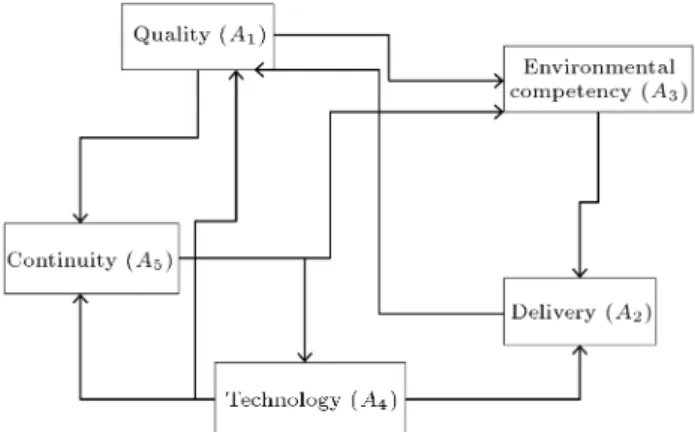
The aim of this paper is to design a resilient supply chain network with focus on SS&OA problem. For this purpose, a two-stage integrated approach is introduced. At the rst stage, the RWs of suppliers are calculated. A set of resilience measurements in the literature is ex-plored and classied into ve categories including qual-ity, delivery, technology, environmental competency, and continuity. Then, trapezoidal fuzzy DEMATEL is applied to nding the strongest interdependencies among dierent measures. Afterwards, triangular fuzzy ANP is used to calculate the RW of supplier (which is known as overall performance of each supplier in the network). At the second stage, a fuzzy multi-objective mixed-integer linear programming model is proposed. The proposed model aims to minimize total cost while maximizing overall performance of the network. Figure 1 shows the proposed integrated approach schematically.
3.1. Problem description
Figure 1. Proposed integrated approach to resilient SS&OA.
have forced organizations to expand their market share for increasing their prot. In order to enhance quality and market share, organizations have to select suppli-ers whose products are of higher quality and lower cost [33]. In fact, organizations should be able not only to produce various products with regard to the needs and preferences of costumers and transport the products to them through resilient and cost-eective networks, but also to purchase the required raw materi-als from ecient suppliers [34]. Possibility of disruption occurrence and the inherent uncertainty of dierent
parameters in supply chain network in real cases add to the complexity of the problem.
This paper considers a three-level supply chain including supplier, manufacturer, and retailer. Suppli-ers supply the required raw materials for production at the level of manufacturers and the nal products are shipped to retailers. Fixed and variable costs are diverse in dierent plants with various technologies and resources. Each manufacturer is capable of producing one or more products. Manufacturers select the suppli-ers and determine order quantity for each raw material.
Table 1. Measures of the resilience of suppliers.
RM Indicator Ref.
A1: Quality
C1: Defect rate [35]
C2: Durability [36]
C3: Strength [37]
C4: Part safety [38]
C5: Reusability [16]
C6: Customer service [38]
A2: Delivery
C7: Lead time [39]
C8: Order fulllment rate [37]
C9: Responsiveness [37]
A3: Environmental
competency
C10: Resource consumption [40]
C11: Environmental management system [29]
C12: Carbon management competency [25]
C13: Green packaging [41]
C14: Reduction in waste [41]
C15: Ecodesign [41]
A4: Technology C16: Capability of R&D [42]
C17: Capability of design [42]
A5: Continuity
C18: Collaboration with other organizations [43]
C19: Risk management culture [44]
C20: Adaptive capability [43]
C21: Strategic risk planning [44]
C22: Information sharing [43]
Type and amount of transferred products from each manufacturer to the retailer should be determined. 3.2. Calculating RW
The main objective of this stage is to obtain RW of suppliers. A list of resilience measures and indicators is explored by reviewing the relevant literature on supplier selection. Table 1 reports the list of resilience measures for resilience measurement of suppliers. The interdependencies among resilience measures and indi-cators are calculated through a hybrid fuzzy MCDM method, which comprises fuzzy DEMATEL and fuzzy ANP methods. Finally, the overall performance of each supplier is calculated from the viewpoint of the interested parties towards suppliers.
In a survey, decision makers or stakeholders of supply chain are asked to score the resilience measures of the suppliers with respect to each indicator in the range of 1 to 9. The nal RW of supplier (i) with
respect to RM l can be calculated by Eq. (1): nli=
" h Y
k=1
nlikMk
!# 1
h P
k=1Mk; (1)
where nlz is the nal score for supplier i with respect
to RM l, nlzk is the score given by stakeholder k for
the resilience of supplier (i) with respect to indicator l, and Mk is the importance of the k-th stakeholder in
the supply chain. Accordingly, the resilience weight of the supplier can be identied by Eq. (2):
OPi = n
X
l=1
nliWfl; (2)
where OPidenotes the RW of supplier i and Wflis the
nal weight of indicator f for RM l, which is calculated by the fuzzy ANP method. A brief explanation of fuzzy DEMATEL and fuzzy ANP methods is provided in Appendix A.
3.3. SS&OA mathematical formulation
The proposed model is formulated as a fuzzy multi-objective mixed-integer linear programming one. It seeks to select the supplier and allocate the order quantity. The RW of the supplier calculated in the previous stage is used as input parameter in the proposed model.
3.3.1. Assumptions
The following assumptions are made to formulate the SS&OA problem:
Planning horizon is divided into certain periods. Decisions are to be made for the beginning of the periods;
Fixed costs and variable costs vary from plant to plant, since the applied equipment and facilities in each plant are dierent. These costs may dier in each period;
Each product is composed of several components the types and quantities of which are specied according to BOM;
For supplying each raw material, one or more suppliers are available;
The manufacturer can purchase excessive materials in one period and transport them to customers after production in the following periods;
The manufacturer may face shortage in a period and compensate for it in the following periods;
Inventory amount and inventory shortage in all plants are zero at the beginning of the planning horizon;
Excess products and shortage of products impose extra costs;
Suppliers may meet demands of the plants in subse-quent periods (shortage is allowed);
Suppliers may produce excessive products in a pe-riod and transport them to plants in the following periods;
Each plant has specied capacity;
Disruption rates for each actor in each period are specied based on experiences and judgments of the experts;
Time is not intended directly for transportation of materials and products. The eect of time is considered as transportation cost.
3.3.2. Notation
The following notation is used to formulate the SS&OA:
Indices
i Index of supplier (i = 1; :::; I) j Index of manufacturer (j = 1; :::; J) k Index of material (k = 1; :::; K) s Index of retailer (s = 1; :::; S) n Index of product (n = 1; :::; N) t Index of period (t = 1; :::; T ) Parameters
~ Pt
jn Production capacity of manufacturer j
for product n in period t ~
Pt
sn Capacity of retailer s for product n in
period t ~
Pt
ik Capacity of supplier i for supplying
material k in period t ~
dt
sn Demand of retailer s for product n in
period t ~
Ct
ijk Transportation cost of material k from
supplier i to manufacturer j in period t ~t
ijk Purchasing cost of material k from
supplier i for manufacturer j in period t
~t
jsn Transportation cost of product n from
manufacturer j to retailer s in period t ~t
jn Variable production cost of product n
in manufacturer j in period t ~qt
j Operational xed cost of manufacturer
j in period t eht
s Operational xed cost of supplier s in
period t
!nk Quantity of material k required to
produce one unit of product n based on BOM
~ut
jn Average disruption rate for
manufacturer j and product n in period t
~vt
sn Average disruption rate for retailer s
and product n in period t ~t
ik Average disruption rate for supplier i
and material k in period t ~
$t
jsn Excessive production cost of product
n in manufacturer j for retailer s in period t
~t
jsn Shortage cost of product n in
manufacturer j for retailer s in period t
~ $0t
ijk Excessive cost of material k from
supplier i for manufacturer s in period t
~t
ijk Shortage cost of material k from
supplier i for manufacturer s in period t
Decision variables xt
ijk Amount of material k ordered by
manufacturer j from supplier i in period t
yt
jsn Amount of product type n transported
from manufacturer j to retailer s in period t
It
jsn Amount of excessive production of
product n by manufacturer j for retailer s in period t
Bt
jsn Amount of shortage in production
of product n by manufacturer j for retailer s in period t
I0t
ijk Amount of excessive purchasing
of material k from supplier i for manufacturer s in period t B0t
ijk Amount of shortage in purchasing
of material k from supplier i for manufacturer s in period t t
ik 1 if supplier i is selected for purchasing
material k in period t; 0, otherwise t
sn 1 if retailer s is selected for selling
product n in period t; 0, otherwise t
jn 1 if manufacturer j is selected for
production product n in period t; 0, otherwise
3.3.3. Problem formulation
The proposed fuzzy multi-objective mixed-integer lin-ear programming model for SS&OA problem is as follows:
Minf1=
X i X j X k ~ Ct
ijk:xtijk+
X i X j X k ~t ijk:xtijk
+X
j
X
s
~t
jsn:ytjsn+
X
j
~t jn:jnt :
X s yt jsn ! +X j ~qt j:tjn+
X
s
eht s:snt
+ T X t=1 J X j=1 S X s=1 N X n=1 (It
jsn: ~$jsnt +Btjsn~tjsn)
+XT
t=1 I X i=1 J X j=1 K X k=1
(I0t ijk: ~$
0t
ijk+B
0t
ijk: ~
0t
ijk); (3)
Maxf2=
X i X j X k
OPi:xtijk; (4)
s.t. X
j
xt
ijk ~Pikt:tik 8i; k; t; (5)
S X s=1 N X n=1 yt jsn N X n=1 ~ Pt
jnjnt 8j; t; (6)
J X j=1 N X n=1 yt jsn N X n=1 ~ Pt
snsnt 8s; t; (7)
I X i=1 K X k=1
!nk:xtijk:(1 ~ikt )
=XS
s=1
(1 ~ut
jn):yjsnt 8j; n; t; (8)
S X s=1 J X j=1
(1 ~ut
jn):ytjsn:tjn
= S X s=1 J X j=1
(1 ~vt
sn):snt :yjsnt 8n; t; (9)
J X j=1 y1 jsn J X j=1 I1 jsn+ J X j=1 B1
jsn d~1sn= 0
8s; n; (10)
J
X
j=1
Ijsn(t 1) XJ
j=1
Bjsn(t 1)+XJ
j=1 yt jsn = J X j=1 It jsn J X j=1 Bt
jsn+ ~dtsn
8s; n; t 2; 3; :::; T; (11)
IT
jsn= BjsnT = 0 8j; s; n; (12)
I0
jsn= Bjsn0 = 0 8j; s; n; (13)
I X i=1 x1 ijk I X i=1 I01 ijk+ I X i=1
B01 ijk N X n=1 !nk S X s=1 y1
I
X
i=1
I0(t 1) ijk
I
X
i=1
B0(t 1) ijk +
I
X
i=1
xt ijk
=
I
X
i=1
I0t ijk
I
X
i=1
B0t ijk+
N
X
n=1
!nk S
X
s=1
yt jsn
8j; k; t 2; 3; :::; T; (15)
I0T
ijk= B0Tijk= 0 8j; k; i; (16)
I00
ijk= B00ijk= 0 8k; i; j; (17)
J
X
j=1
(1 ~ut
jn):ytjsn:tjn= (1 ~vsnt ): ~dtsn:snt
8s; t; n; (18)
xt
ijk; yjsnt ; Ijsnt ; Bjsnt ; I0tijk; B0tijk2
8i; j; k; s; t; n; (19)
t
ik; snt ; tjn2 f0; 1g 8i; j; k; s; n; t: (20)
The objective f1 is to minimize total cost of supply
chain, consisting of material transportation cost (from suppliers to plants), material purchasing cost (by man-ufacturer from supplier), product transportation cost (from manufacturer to retailers), variable production cost, and xed costs (both manufacturer and retailer). The problem is multi-period and close relation exists between supplier and manufacturer in dierent periods. Hence, the last two terms of f1 are considered as
penalty costs for excessive material and shortage in supply and production. The objective f2is to maximize
resilience in the performance of the network. The function is calculated by multiplying resilience weight (derived in the rst stage) by the amount of order for each supplier. It helps the model to select suppliers with higher RW and increase the resilience level of the supply chain network. Eqs. (6) to (8) guarantee the capacities of suppliers, plants, and retailers in each period, respectively. As the problem is a three-level supply chain network, two balance equations are formulated. Eqs. (9) and (10) are balance equations between suppliers and manufacturers, and between plants and retailers, respectively. Since excessive products and materials and shortage at the levels of plants and suppliers are considered in the problem, two mid-term balance equations are developed for products and materials. Eq. (11) ensures balance between all products and retailers with shortage in production or excessive production during the rst period. Eq. (12) transforms excess products and shortages from a period to the subsequent one. Eqs. (13) and (14) ensure that
the amounts of excess and shortage are zero at the beginning and end of the planning horizon. Eqs. (11) to (14) are balance constraints for excess and shortage of products. Similarly, Eqs. (15) to (18) are balance constraints for excess and shortage of materials. Each retailer may order a specic amount of each product from the manufacturer in each period based on the demands of their customers. Demand equation is formulated in terms of disruption rates and demands of retailers in Eq. (19). Finally, Eqs. (20) and (21) enforce integer and binary restrictions on the corresponding decision variables.
4. Solution methodology
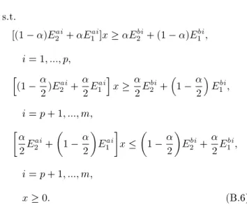
To cope with the uncertainty and multi-objectives of the proposed SS&OA model, a two-phase approach is used. In the rst phase, the methods of Jimenez et al. [45] and Parra et al. [46] are hybridized, as suggested by Pishvaee and Torabi [47], to convert the model into an equivalent auxiliary crisp one. Then, in the second phase, the Torabi-Hassini (TH) method [48] is applied to nding the preferred nal compromise so-lution. For the sake of more clarity, the transformation method [47] is introduced in Appendix B.
In the equivalent crisp model achieved in the previous section, the following steps should be taken to nd the preferred compromise solution:
Step 1: Determine the Positive Ideal Solution (PIS) and Negative Ideal Solution (NIS) for each objective function by solving the corresponding MILP model.
fP IS
1 = min f1; f1NIS= max f1;
fP IS
2 = max f2; f2NIS= min f2:
In order to reduce computational complexity, the fol-lowing rules have been suggested in TH method [48]: Obtaining an approximate PIS for each objec-tive function by solving the corresponding MILP heuristically to obtain a satisfactory feasible inte-ger solution;
Instead of solving a separate MILP for determining each NIS, we can estimate them using the PISs. Let v
and f(v) denote the decision vector
asso-ciated with the PIS of the th objective function and the corresponding value, respectively. Thus, the related NIS could be estimated as follows:
fNIS
= minff1(v1); f2(v2); f3(v3)g:
Step 2: Specify a linear membership function for each objective function as follows:
1(x) =
8 > < > :
1 if f1< f1P IS fNIS
1 f1
fNIS
1 f1P IS if f
P IS
1 f1 f1NIS
0 if f1> f1NIS
2(x) =
8 > < > :
1 if f2< f2P IS f2 f2NIS
fP IS
2 f2NIS if f
NIS
2 f2 f2P IS
0 if f2> f2NIS
(22) Step 3: Convert the model into an equivalent single-objective function using the following formulation:
max (v) = 0+ (1 )(11(v) + 22(v));
s.t.:
0 1(v); 0 1(v);
v 2 F (v); ; 02 [0; 1]; (23)
where (v) and 0 = minf(v)g denote the
satisfaction degree of the th objective function and the minimum satisfaction degree of objectives, respectively. This formulation has a new achievement function dened as a convex combination of the lower bound for satisfaction degree of objectives (0)
and the weighted sum of these achievement degrees ((v)) to ensure yielding an adjustable balanced
compromise solution. Also, and indicate the
relative importance of the th objective function and the coecient of compensation. is determined by
the decision maker based on their preferences so that 1+2= 1. Also, controls the minimum satisfaction
level of objectives as well as the compromise degree among the objectives. implicitly.
Step 4: Solve the crisp model by the MIP solver. If the decision maker is satised with the current ecient compromise solution, stop. Otherwise, pro-vide another ecient solution by changing the values of controllable parameters and , and go back to Step 1.
5. Case study
In order to illustrate the application of the proposed integrated approach to supply chain network design, the case study of a wood products manufacturer in northern Iran is presented. The company produces
wooden buet and chest of drawers in two workshops. The main raw material for each product is MDF sheet with specic thickness and width. According to the Bill Of Materials (BOM), the required amount of materials for each product is shown in Table 2. Inventory cost and cost of shortages for each work-shop are assumed to be common. Cost of excessive production and cost of shortage in production are triangular fuzzy numbers with uniform distribution as (p = U[5000; 8000]; m = U[9000; 12000]; o = U [15000; 20000]) and (p = U[80000; 100000], m = U [120000; 150000], o = [180000; 200000]), respectively.
The company can obtain the required raw ma-terials from three suppliers (Sup1, Sup2, Sup3). As
stated before, the company has two workshops for manufacturing the products. The required data for each workshop are shown in Table 3. Moreover, three planning periods are considered. Since the two workshops are located in the same industrial zone, their transportation and purchasing costs are the same. In this case, three retailers are considered. The required data for one of the retailers are presented in Table 4 and the remainder are omitted for brevity. Three experts expressed their opinions about the suppliers of the company and the interdependencies among the MAs and the overall performance of suppliers were calculated based on their quoted data. The network derived from DEMATEL is shown in Figure 2 and
Figure 2. The network derived from DEMATEL.
Table 2. Required amount of materials for each product. Product (n) Raw material (k) Required amount Chest of drawers (n = 1)
MDF 16 mm (k = 1) 73000 cubic centimeters MDF 3 mm (k = 2) 6900 cubic centimeters Lace wood (k = 3) 8
Wooden buet
MDF 16 mm (k = 1) 61950 cubic centimeters MDF 25 mm (k = 4) 16852 cubic centimeters Lace wood (k = 3) 14
Table 3. Data for workshops.
Workshop Operational xed cost Product Parameter Period Period q~t
j 1 2 3
1
1 (Oct)
p = U[50; 55] m = U[42; 50]
Chest of drawers
Capacity ( ~Pt
jn)
(16,20,24) (8,18,22) (12,16,20)
o = U[35; 42]
Variable production
cost (~t jn)
(30,35,40) (25,30,35) (27,32,37)
2 (Nov)
p = U[46; 51] m = U[39; 46]
Average disruption rate (~ut
jn)
(0.2,0.25,0.3) (0.3,0.35,0.4) (0.2,0.25,0.3)
o = U[31; 36]
Wooden buet
Capacity ( ~Pt
jn)
(25,30,35) (10,14,16) (14,16,18)
3 (Dec)
p = U[48; 53]
Variable production
cost (~t jn)
(55,60,65) (50,55,60) (52,57,62)
m = U[37; 48] o = U[32; 39]
Average disruption rate (~ut
jn)
(0.2,0.25,0.3) (0.3,0.35,0.4) (0.2,0.25,0.3)
2
1 (Oct)
p = U[33; 37]
Chest of drawers
Capacity ( ~Pt
jn)
(24,28,32) (4,8,12) (8,12,16) m = U[25; 39]
o = U[23; 28]
Variable production
cost (~t jn)
(25,30,35) (20,25,30) (22,27,32)
2 (Nov)
p = U[28; 34] m = U[22; 32]
Average disruption rate (~ut
jn)
(0.1,0.2,0.25) (0.1,0.2,0.25) (0.1,0.2,0.25)
o = U[19; 24]
Wooden buet
Capacity ( ~Pt
jn)
(10,14,16) (4,10,12) (4,7,8)
3 (Dec)
p = U[31; 36] m = U[24; 34]
Variable production
cost (~t jn)
(65,70,75) (60,65,70) (62,67,72)
o = U[21; 25]
Average disruption rate (~ut
jn)
(0.1,0.2,0.25) (0.1,0.2,0.25) (0.1,0.2,0.25)
Table 4. Partial data for retailers.
Operational xed cost Product Parameter Period Retailer Period $~t
jsn 1 2 3
1
1 (Oct)
p = U[3; 4]
Chest of drawers
Capacity ( ~Pt
sn) (3,5,6) (4,5,6) (4,6,7)
m = U[5; 6]
o = U[7; 8] Demand ( ~dt
sn) (7,8,10) (8,10,12) (8,10,12)
2 (Nov)
p = U[4; 5] Transportation cost (~t
jsn)
(18,25,30) (18,25,30) (18,25,30) m = U[6; 7]
o = U[8; 10] 3 (Dec)
p = U[3; 4] Average
disruption rate ( ~vt
sn)
(.02,.04,.08) (.02,.04,.08) (.02,.04,.08) m = U[6; 7]
Table 5. Partial data for suppliers.
Suppliers Overall Parameter Raw material
performance 1 2 3 4 5
1 6.1812
Purchasing (~t
ijk)
(28,30,35) (3,5,6) (2,4,10) (50,55,60) (1200,1300,1400) Transportation
( ~Ct
ijk) (3,5,7) (1,2,3) (1,2,3) (6,8,10) (20,30,50)
Disruption rate ( ~t
ik)
(0.08,0.1,0.12) (0.08,0.1,0.12) (0.08,0.1,0.12) (0.08,0.1,0.12) (0.08,0.1,0.12)
2 2.643
Purchasing (~t
ijk)
(26,28,33) (2,4,6) (3,4,8) (45,50,52) (1100,1150,1250) Transportation
( ~Ct
ijk) (2,4,8) (1,2,3) (3,3,5) (8,9,12) (22,36,55)
Disruption rate (~t
ik)
(0.1,0.12,0.15) (0.1,0.12,0.15) (0.1,0.12,0.15) (0.1,0.12,0.15) (0.1,0.12,0.15)
3 4.325
Purchasing (~t
ijk)
(32,35,38) (5,7,8) (2,3,5) (52,60,65) (1400,1500,1600) Transportation
( ~Ct
ijk) (6,7,8) (3,4,5) (1,2,3) (9,11,13) (25,35,46)
Disruption rate (~t
ik)
(0.02,0.05,0.1) (0.02,0.05,0.1) (0.02,0.05,0.1) (0.02,0.05,0.1) (0.02,0.05,0.1)
Table 6. Acceptable results for decision makers in the company based on the proposed approach.
Period Workshop Raw material
Supplier
Total cost of purchasing
material
Total cost of transporting
materials Product Retailer
Total production
cost
Total cost of transporting
products
1 2 3 1 2 3
1
1
1 18400 15335 0 98130 153460 Chest of
drawers 3 3 5 3520000 335000
2 16290 2176 0 90750 41252
3 89 0 273 1174 71 Wooden
buet 6 5 5 9120000 612000
4 4826 4021 0 257390 40218
5 269 224 0 163555 25640 Sum 9 8 10 12640000 947000
2
1 0 0 20700 724500 144900 Chest of
drawers 5 5 7 4590000 545000
2 0 2430 8640 70200 39420
3 109 128 0 948 602 Wooden
buet 5 4 3 8040000 455000
4 0 637 2265 18413 10340
5 0 0 303 120750 24150 Sum 10 9 10 12630000 100000
2
1
1 22080 18402 0 1177485 184152 Chest of
drawers 4 4 5 4160000 410000
2 19548 2611 0 108900 49502
3 106 0 327 1408 85 Wooden
buet 8 4 5 9690000 640000
4 5791 4825 0 308868 48261
5 322 268 0 196266 30768 Sum 12 8 10 13850000 1050000
2
1 0 16560 0 579600 115920 Chest of
drawers 6 6 7 5130000 605000
2 1944 0 6912 56160 31536
3 0 87 102 758 481 Wooden
buet 4 3 2 6030000 340000
4 509 0 1812 14730 8272
5 242 0 0 96600 19320 Sum 10 9 9 11160000 945000
3
1
1 0 0 24840 869400 173880 Chest of
drawers 4 4 5 4150000 410000
2 0 2916 10368 84240 47304
3 130 153 0 1137 722 Wooden
buet 7 4 6 9710000 645000
4 0 764 2718 22095 12408
5 0 0 363 144900 28980 Sum 11 8 11 13860000 1050000
2
1 14720 12268 0 785064 122768 Chest of
drawers 6 6 7 5120000 620000
2 13032 1740 0 72600 33001
3 71 0 218 940 57 Wooden
buet 4 5 3 80500000 460000
4 3860 3216 0 205912 32174
5 215 179 0 130844 20512 Sum 10 11 10 13170000 1080000
the overall performance of each supplier is shown in Table 5. Other information including capacity, average disruption rate, and purchasing and transportation costs are shown in Table 5.
The presented model is solved based on dierent
minimum acceptable possibility levels () as well as dierent values of and . Acceptable results for
decision makers in the company are calculated with 1 = 0:8, 1= 0:2, = 0:7, and = 0:6. The results
6. Conclusion
In this paper, an integrated model for supplier selec-tion and order allocaselec-tion was proposed focusing on a dynamic multi-period, multi-sourcing, and multi-item supply chain. Resilience Weights (RWs) of suppli-ers were obtained based on the explored Resilience Measures through a hybrid fuzzy Decision Making Trial and Evaluation Laboratory (DEMATEL) and ANP method. The results were incorporated in a fuzzy multi-objective mixed-integer linear program-ming model. The proposed mathematical model was aimed at minimizing the total cost while maximizing the resilience performance of the supply chain network. The applicability and usefulness of the proposed ap-proach was examined through the real case study of a wood manufacturer company with two workshops, three suppliers, and three retailers. Based on opinions of decision makers, the results were applicable to supply chain network design and it could help them make a balance between supply and market.
Future research could address the inherent uncer-tainty of the problem by dierent approaches such as mixed fuzzy stochastic problems. Furthermore, propos-ing disruption factors and their eects on network structures in the model can lead to a more practical approach. In addition, developing heuristic and meta-heuristic methods for solving large-scale problems is another avenue for the further research.
References
1. Amirtaheri, O., Zandieh, M., and Dorri, B. \A bi-level programming model for decentralized manufacturer-distributer supply chain considering cooperative adver-tising", Scientia Iranica, 25(2), pp. 891{910 (2018). 2. Golp^Ira, H., Zandieh, M., Naja, E., and Sadi-Nezhad,
S. \A multi-objective multi-echelon green supply chain network design problem with risk-averse retailers in an uncertain environment", Scientia Iranica, Transaction E, Industrial Engineering, 24(1), pp. 413{423 (2017). 3. Sahebjamnia, N., Tavakkoli-Moghaddam, R., and
Ghorbani, N. \Designing a fuzzy Q-learning multi-agent quality control system for a continuous chemical production line-A case study", Computers & Industrial Engineering, 93, pp. 215{226 (2016).
4. Jafari, H.R., Seifbarghy, M., and Omidvari, M. \Sus-tainable supply chain design with water environmental impacts and justice-oriented employment considera-tions: A case study in textile industry", Scientia Iranica, 24(4). pp. 2119{2137 (2017).
5. Rao, C.J., Zheng, J.J., Hu, Z., and Goh, M., \Com-pound mechanism design on attribute and multi-source procurement of electricity coal", Scientia Iran-ica, 23(3), pp. 1384{1398 (2016).
6. Torkaman, S., Ghomi, S.F., and Karimi, B. \Multi-stage multi-product multi-period production planning
with sequence-dependent setups in closed-loop supply chain", Computers & Industrial Engineering, 113, pp. 602{613 (2017).
7. Bashiri, M. and Hasanzadeh, H. \Modeling of location-distribution considering customers with dierent pri-orities by a lexicographic approach", Scientia Iranica, 23(2), pp. 701{710 (2016).
8. Hlioui, R., Gharbi, A., and Hajji, A. \Joint supplier se-lection, production and replenishment of an unreliable manufacturing-oriented supply chain", International Journal of Production Economics, 187, pp. 53{67 (2017).
9. Mahdavi, I., Shirazi, B., and Sahebjamnia, N. \De-velopment of a simulation-based optimisation for con-trolling operation allocation and material handling equipment selection in FMS", International Journal of Production Research, 49(23), pp. 6981{7005 (2011). 10. Gharaei, A., Pasandideh, S.H.R., and Akhavan Niaki,
S.T. \An optimal integrated lot sizing policy of in-ventory in a bi-objective multi-level supply chain with stochastic constraints and imperfect products", Jour-nal of Industrial and Production Engineering, 35(1), pp. 6{20 (2018).
11. Alfares, H.K. and Turnadi, R. \Lot sizing and sup-plier selection with multiple items, multiple periods, quantity discounts, and backordering", Computers & Industrial Engineering, 116, pp. 59{71 (2018). 12. Sahebjamnia, N., Torabi, S.A., and Mansouri, S.A.
\Building organizational resilience in the face of mul-tiple disruptions", International Journal of Production Economics, 197, pp. 63{83 (2018).
13. Scheibe, K.P. and Blackhurst, J. \Supply chain dis-ruption propagation: a systemic risk and normal accident theory perspective", International Journal of Production Research, 56(1{2), pp. 43{59 (2018). 14. Aissaoui, N., Haouari, M., and Hassini, E. \Supplier
selection and order lot sizing modeling: A review", Computers & Operations Research, 34(12), pp. 3516{ 3540 (2007).
15. Hajikhani, A., Khalilzadeh, M., and Sadjadi, S.J. \A fuzzy multi-objective multi-product supplier selection and order allocation problem in supply chain under coverage and price considerations: An urban agricul-tural case study", Scientia Iranica, 25(1), pp. 431{449 (2018).
16. Govindan, K., Rajendran, S., Sarkis, J., and Muruge-san, P. \Multi criteria decision making approaches for green supplier evaluation and selection: a literature review", Journal of Cleaner Production, 98, pp. 66{83 (2015).
17. Babbar, C. and Amin, S.H. \A multi-objective mathe-matical model integrating environmental concerns for supplier selection and order allocation based on fuzzy QFD in beverages industry", Expert Systems with Applications, 92, pp. 27{38 (2018).
18. Fallahpour, A., Olugu, E.U., and Musa, S.N. \A hybrid model for supplier selection: integration of AHP and
multi expression programming (MEP)", Neural Com-puting and Applications, 28(3), pp. 499{504 (2017). 19. Hammami, R., Temponi, C., and Frein, Y. \A
scenario-based stochastic model for supplier selection in global context with multiple buyers, currency uc-tuation uncertainties, and price discounts", European Journal of Operational Research, 233(1), pp. 159{170 (2014).
20. Goren, H.G. \A decision framework for sustainable supplier selection and order allocation with lost sales", Journal of Cleaner Production, 183, pp. 1156{1169 (2018).
21. Chai, J., Liu, J.N., and Ngai, E.W. \Application of decision-making techniques in supplier selection: A systematic review of literature", Expert Systems with Applications, 40(10), pp. 3872{3885 (2013).
22. Mahmoudi, A., Sadi-Nezhad, S., and Makui, A. \An extended fuzzy VIKOR for group decision making based on fuzzy distance to supplier selection", Scientia Iranica, 23(4), pp. 1879{1892 (2016).
23. Keshavarz Ghorabaee, M., Amiri, M., Zavadskas, E.K., and Antucheviciene, J. \Supplier evaluation and selection in fuzzy environments: a review of MADM approaches", Economic Research-Ekonomska Istrazivanja, 30(1), pp. 1073{1118 (2017).
24. Rezaei, J. and Davoodi, M. \Multi-objective models for lot-sizing with supplier selection", International Journal of Production Economics, 130(1), pp. 77{86 (2011).
25. Govindan, K., Fattahi, M., and Keyvanshokooh, E. \Supply chain network design under uncertainty: A comprehensive review and future research directions", European Journal of Operational Research, 263(1), pp. 108{141 (2017).
26. Tabibian, M. and Rezapour, M. \Assessment of urban resilience; a case study of Region 8 of Tehran city, Iran", Scientia Iranica, 23(4), pp. 1699{1707 (2016). 27. Bidokhti, A.A., Shariepour, Z., and Sehatkashani,
S. \Corrigendum to some resilient aspects of urban areas to air pollution and climate change, case study: Tehran, Iran", Scientia Iranica, 23(6), pp. 1994{2004 (2016).
28. Hsieh, C.Y., Wee, H.M., and Chen, A. \Resilient logistics to mitigate supply chain uncertainty: A case study of an automotive company", Scientia Iranica, 23(5), pp. 2287{2296 (2016).
29. Khaloo, A.R. and Mobini, M.H. \Towards resilient structures", Scientia Iranica, 23(5), pp. 2077{2080 (2016).
30. Sawik, T., \Selection of resilient supply portfolio under disruption risks", Omega, 41(2), pp. 259{269 (2013).
31. Fattahi, M. \Resilient procurement planning for sup-ply chains: A case study for sourcing a critical mineral material", Resources Policy (In press) (2017). https://doi.org/10.1016/j.resourpol.2017.10.010 32. Vahidi, F., Torabi, S.A., and Ramezankhani, M.J.
\Sustainable supplier selection and order allocation under operational and disruption risks", Journal of Cleaner Production, 174, pp. 1351{1365 (2018). 33. Taleizadeh, A.A., Niaki, S.T.A., and Barzinpour, F.
\Multiple-buyer multiple-vendor product multi-constraint supply chain problem with stochastic de-mand and variable lead-time: A harmony search algorithm", Applied Mathematics and Computation, 217(22), p. 9234{9253 (2011).
34. Sahebjamnia, N., Torabi, S.A., and Mansouri, S.A. \Integrated business continuity and disaster recovery planning: Towards organizational resilience", Euro-pean Journal of Operational Research, 242(1), pp. 261{273 (2015).
35. Torabi, S., Baghersad, M., and Mansouri, S. \Resilient supplier selection and order allocation under opera-tional and disruption risks", Transportation Research Part E: Logistics and Transportation Review, 79, pp. 22{48 (2015).
36. Gaur, J., Subramoniam, R., Govindan, K., and Huis-ingh, D. \Closed-loop supply chain management: From conceptual to an action oriented framework on core acquisition", Journal of Cleaner Production, 30, pp. 1{10 (2016).
37. Namdar, J., Tavakkoli-Moghaddam, R., Sahebjamnia, N., and Sou, H.R. \Designing a reliable distribution network with facility fortication and transshipment under partial and complete disruptions", International Journal of Engineering-Transactions C: Aspects C, 29(9), pp. 1273{1281 (2016).
38. Tukamuhabwa, B.R., Stevenson, M., Busby, J., and Zorzini, M. \Supply chain resilience: denition, review and theoretical foundations for further study", Inter-national Journal of Production Research, 53(18), pp. 5592{5623 (2015).
39. Altiparmak, F., Gen, M., Lin, L., and Paksoy, T., \A genetic algorithm approach for multi-objective optimization of supply chain networks", Computers & Industrial Engineering, 51(1), pp. 196{215 (2006). 40. Vahidi, F., Torabi, S.A., and Ramezankhani, M.
\Sustainable supplier selection and order allocation under operational and disruption risks", Journal of Cleaner Production, 174, pp. 1351{1365 (2018). 41. Awasthi, A., Govindan, K., and Gold, S.
\Multi-tier sustainable global supplier selection using a fuzzy AHP-VIKOR based approach", International Journal of Production Economics, 195, pp. 106{117 (2018).
42. Soosay, C.A., Hyland, P.W., and Ferrer, M. \Supply chain collaboration: capabilities for continuous inno-vation", Supply Chain Management: An International Journal, 13(2), pp. 160{169 (2008).
43. Torabi, S.A., Rezaei Sou, H., and Sahebjamnia, N. \A new framework for business impact analysis in business continuity management (with a case study)", Safety Science, 68, pp. 309{323 (2014).
44. Torabi, S.A., Giahi, R., and Sahebjamnia, N. \An enhanced risk assessment framework for business con-tinuity management systems", Safety Science, 89, pp. 201{218 (2016).
45. Jimenez, M., Arenas, M., Bilbao, A., and Rodr, M.V. \Linear programming with fuzzy parameters: an interactive method resolution", European Journal of Operational Research, 177(3), pp. 1599{1609 (2007). 46. Parra, M.A., Terol, A.B., Gladish, B.P., and Ura,
M.R. \Solving a multiobjective possibilistic problem through compromise programming", European Journal of Operational Research, 164(3), pp. 748{759 (2005). 47. Pishvaee, M. and Torabi, S. \A possibilistic
program-ming approach for closed-loop supply chain network design under uncertainty", Fuzzy Sets and Systems, 161(20), pp. 2668{2683 (2010).
48. Torabi, S.A. and Hassini, E. \An interactive possibilis-tic programming approach for multiple objective sup-ply chain master planning", Fuzzy Sets and Systems, 159(2), pp. 193{214 (2008).
49. Liou, James J.H. \Developing an integrated model for the selection of strategic alliance partners in the airline industry", Knowledge-Based Systems, 28, pp. 59{67 (2012).
50. Tzeng, G.-H., Chiang, C.-H., and Li, C.-W. \Eval-uating intertwined eects in e-learning programs: A novel hybrid MCDM model based on factor analysis and DEMATEL", Expert Systems with Applications, 32(4), pp. 1028{1044 (2007).
51. Suo, W.-L., Feng, B., and Fan, Z.-P. \Extension of the DEMATEL method in an uncertain linguistic environment", Soft Computing, 16(3), pp. 471{483 (2012).
52. Hiete, M., Merz, M., Comes, T., and Schultmann, F. \Trapezoidal fuzzy DEMATEL method to analyze and correct for relations between variables in a composite indicator for disaster resilience", OR Spectrum, 34(4), pp. 971{995 (2012).
53. Li, C.-W. and Tzeng, G.-H. \Identication of a threshold value for the DEMATEL method using the maximum mean de-entropy algorithm to nd critical services provided by a semiconductor intellectual prop-erty mall", Expert Systems with Applications, 36(6), pp. 9891{9898 (2009).
54. Saaty, T.L., Decision Making with Dependence and Feedback: The Analytic Network Process, Pittsburgh, RWS Publications (1996).
55. Yang, J.L. and Tzeng, G.-H. \An integrated MCDM technique combined with DEMATEL for a novel cluster-weighted with ANP method", Expert Systems with Applications, 38(3), pp. 1417{1424 (2011). 56. Jimenez, M. \Ranking fuzzy numbers through the
comparison of its expected intervals", International Journal of Uncertainty, Fuzziness and Knowledge-Based Systems, 4(04), pp. 379{388 (1996).
Appendix A DEMATEL
DEMATEL method has successfully been applied to dierent areas such as e-learning, marketing strategy, service quality, safety problems, and supplier selection [21,49]. DEMATEL method was founded based on graph theory. It uses matrix calculation to visualize the problem and calculate impact strength of existing relations [50]. In this paper, trapezoidal fuzzy DE-MATEL is applied to mapping the interdependencies among MAs and nding the corresponding impact strength. Fuzzy trapezoidal numbers are expressed as follows [51]:
e
dlu=(d1lu; d2lu; d3lu; d4lu) =
max
2l 1 2g + 1; 0
; 2l
2g + 1; 2u + 1 2g + 1; min
2u + 2
2g + 1; 1 ; (A.1) where l, u, and g can be obtained according to the following denitions:
Denition 1. Let S = fs0; si; :::sgg be a nite and
totally ordered set, where sl is the ith linguistic term,
i 2 f0; 1; :::; gg. Then, S is called the linguistic term set and g + 1 the cardinality of S.
Denition 2. Considering bS = fsl; sl+1; :::sug,
where sl and su are the lower and upper limits,
re-spectively, and l; u 2 f0; 1; :::; gg, bS is called uncertain linguistic term, which can be expressed as [sl; su]; u l
indicates the degree of fuzziness.
This paper takes the following fuzzy DEMATEL steps provided by Suo et al. and Hiete et al. [51,52] to map the interdependencies among MAs:
Step 1. Ask a committee of experts to express their viewpoints towards the relations between MAs with uncertain linguistic terms and calculate the average matrix;
Step 2. Calculate the total relation matrix based on the normalized initial direct relation matrix acquired from the average matrix.
Step 3. Dene a threshold value to construct impact relation map. In this paper, threshold value is dened
by the experts. However, there are some algorithms such as mean de-entropy (MMDE) developed by Li and Tzeng [53] to set a proper threshold value. Step 4. Map the interdependencies among MAs based on the total relation matrix and the dened threshold value.
Fuzzy ANP
ANP, which was introduced by Saaty [54], includesall possible connections between elements and is a general form of the top to bottom hierarchy in AHP. In this paper, fuzzy ANP is applied to capturing the viewpoints of experts towards dierent KPIs through pairwise comparisons to nd the weight of each KPI. According to the previous step, each Ma may aect the other one dierently. Therefore, the cluster weighting proposed by Yang and Tzeng [55] is applied in this paper to incorporating the DEMATEL results in the fuzzy ANP method. The fuzzy ANP steps are as follows:
Step 1. Develop unweighted supermatrix through pairwise comparisons using fuzzy triangular numbers based on Table A.1;
Step 2. Calculate the weighted supermatrix via mul-tiplying the derived matrix from DEMATEL method by defuzzied unweighted supermatrix;
Step 3. Rise the weighted supermatrix to limiting power to acquire global priority vectors, which are weights of KPIs denoted by Wf.
Appendix B
Auxiliary crisp model
The Expected Interval (EI) and Expected Value (EV) of the triangular fuzzy number ea T F N (ap; am; ao)
can be dened as follows [56]: EI(ea) = [Ea
1; E2a]
= Z 1
0 f 1 a (x)dx;
Z 1
0 g 1 a (x)dx
=
1
2(ap+ am); 1
2(am+ ao)
; (B.1)
Table A.1. Linguistic terms and the equivalent fuzzy numbers.
Linguistic term Membership function Equally important (1; 1; 3)
Moderately important (1; 3; 5)
Important (3; 5; 7)
Very important (5; 7; 9) Extremely important (7; 9; 9)
EV (ea) = E1a+ E2 2a = ap+ 2a4m+ ao: (B.2) According to Jimenez et al. [45], the equivalent crisp equations for eaix ebi and eaix = ebi are the following,
respectively:
(1 ) Eai
2 + E1ai
x Ebi
2 + (1 ) E1bi; (B.3)
h
1 2Eai
2 +2E1ai
i
x 2Ebi 2 +
1 2Ebi 1;
h 2E2ai+
1 2Eai 1
i
x1 2Ebi
2 +2E1bi; (B.4)
where is the minimum acceptable possibility level for imprecise parameters.
Now, consider the following fuzzy mathematical programming model:
min z = ectx
s.t.:
eaix ebi; i = 1; :::; p;
eaix = ebi; i = p + 1; :::; m;
x 0: (B.5)
Based on the denitions of expected value and expected interval, the equivalent crisp model for the above formulation is as follows:
min z = EV (ec)x s.t.
[(1 )Eai
2 + E1ai]x E2bi+ (1 )E1bi;
i = 1; :::; p; h
(1 2)Eai
2 +2E1ai
i
x 2Ebi 2 +
1 2Ebi 1;
i = p + 1; :::; m;
2E2ai+
1 2
Eai
1
x
1 2
Ebi
2 +2E1bi;
i = p + 1; :::; m;
x 0: (B.6)
Biography
Navid Sahebjamnia is an Assistant Professor of Industrial and System Engineering in the Department of Industrial Engineering at University of Science and Technology of Mazandaran. He specializes in applying novel management science and operations
research methods to business decision-making prob-lems, focusing on current trends and issues in sup-ply chain management and addressing them by us-ing multiple-criteria decision makus-ing techniques and uncertainty programming approaches. His main re-search interests include commercial and humanitarian supply chain, organizational and urban resilience, sus-tainable operations management, disaster operations
management, healthcare operations management, and strategic management. Dr. Sahebjamnia has published several papers in accredited scientic journals such as International Journal of Production Economics, European Journal of Operational Research, Decision Support Systems, International Journal of Production Research, Computers and Industrial Engineering, and Knowledge-Based Systems.

![Table 1. Measures of the resilience of suppliers. RM Indicator Ref. A 1 : Quality C 1 : Defect rate [35]C2: Durability[36]C3: Strength[37] C 4 : Part safety [38] C 5 : Reusability [16] C 6 : Customer service [38] A 2 : Delivery C 7 : Lead time [39]](https://thumb-us.123doks.com/thumbv2/123dok_us/8365221.2221599/5.892.223.692.168.778/measures-resilience-suppliers-indicator-durability-strength-reusability-customer.webp)