PREDICTING STUDENTS«¤?? ENROLLMENT USING GENERALIZED FEED-FORWARD NEURAL NETWORK

PREDICTING STUDENTS’ ENROLLMENT USING

GENERALIZED FEED-FORWARD NEURAL NETWORK

1_{F.A. RUFAI}2 _{O. FOLORUNSO AND} 1 _{O.L. USMAN}

1_{Department of Computer Science, Tai Solarin University of Education, Ogun State}

Nigeria

2_{Department of Computer Science, Federal University of Agriculture, Abeokuta,}

Nigeria.

*Corresponding author: [email protected]; Tel: +234(0) 8062344746

projections which forms the basis for many of the investment decisions. According to Guo (2002), enrollment projection provides information for decision making and budget planning. However, obtaining accuracy is not an easy task, as many factors have impacts on the enrollment numbers. For instance, factors like school fees, politics, quality of teaching (facilities), strike and security may affect the accuracy and reliability of students’ enrollment prediction in Nigeria higher

ABSTRACT

An important obligation of educational planning is the projection of students’ enrollment which forms the basis for many of the investment decisions. Enrollment projection provides information for decision making and budget planning hence, it is important to the development of higher education. As many factors have impacts on the enrollment number, and for the above reasons, students’ population and enrollment number should be considered as a chaotic system. In this research, a Generalized

Feed-Forward Neural Network (GFFNN) for students’ enrollment prediction was proposed. The

architec-ture of the proposed model was in-line with eight steps involved in developing a neural network model for predicting a chaotic system. The data used was obtained from Academic Planning and Quality Control Unit of Tai Solarin University of Education, Ogun State Nigeria. The results from the study showed that the mean absolute percent error of GFFNN has an average of 0.0101% unlike linear re-gression and autorere-gression models that were compared with it, with an average of 0.0570% and 0.0725% respectively. The proposed methodology is expected to assist the school management to adequately plan for the future needs of the students in the provision of facilities.

Key words: Students’ Enrollment, Generalized Feed-Forward Neural Network, Prediction, Higher Education, Regression

INTRODUCTION

Planned economic development requires data about various aspects of socio-economic conditions at different levels. In-dicators of development are directly or indi-rectly related to the size and structure of the population. It is, therefore, of paramount importance to know various aspects of the size and structure of population at different points in time. Another important require-ment of educational planning is enrollrequire-ment

Science, Engineering and Technology

Print - 2277 - 0593 Online - 2315 - 7461 © FUNAAB 2015

institutions of learning. Consequently, stu-dents’ population and enrollment number should be considered as a chaotic system. In this case, some small change in one of the conditioning factors may bring in a sizeable change in the enrollment figure of students at a given point in time.

Methods such as statistical procedures, con-ventional mathematical and artificial intelli-gence (AI) techniques have been used in enrollment projection. Different methods generate different error terms, which are often converted to a percentage so that er-ror terms from different models can be used for comparison in order to determine which model produces optimal results for modelling the time-series of student enroll-ment. For example, Guo (2002) applied re-gression, autoregression, and three-component models to predict the year 2000 students’ enrollments of six community col-leges in California using 1992-1999 popula-tion informapopula-tion from the Department of Finance as impact factors. These techniques generated errors ranging from 0.08% to 4.87% with an average error of 3.03%. Song and Chissom (1993) applied the fuzzy time-series model and neural network ap-proaches to predict university students’ en-rollments and the results found to be satis-factory than the equivalent statistical and mathematical methods. Keilman, et al, (2002) and as also, Bandyopadhyay and Chattopadhyay (2008) stated that statistical approaches are not very suitable for predict-ing a chaotic system like students’ enroll-ment because they make assumptions, which are sometimes found unrealistic and cannot deal with the intrinsic chaos.

Artificial Neural Network (ANN) is found to be useful in the situations where underlying processes and relationships may display chaotic properties. Its applications

have been felt in the tasks involving pattern recognition, classification, and time-series forecasting. ANN does not require any prior knowledge of the system under considera-tion and as well suited to model dynamic systems on a real time basis. Unlike statistical and mathematical techniques which depend on influencing factors, the success of ANN prediction accuracy depends on parameters adjustment (Kaastra & Boyd, 1996; Maqsood

et al., 2002). Therefore, ANN was applied to

predict the future enrollment of students in the four colleges of Tai Solarin University of Education, Ogun State Nigeria using data obtained from Academic Planning and Qual-ity Control Unit of the universQual-ity (2013). Model was built using a Generalized Feed-Forward Neural Network (GFFNN), and its prediction accuracy is compared with Linear Regression (LR) and Autoregression (AR) which have been the popular statistical meth-ods of population projection over the years.

STATEMENT OF THE

PROBLEM

The changes in student population necessi-tate deep insights in enrollment projection. With the increasing changes in technology and the increased demands for various com-petencies and collaboration among employ-ees, people of diverse ages feel the necessity to obtain more education. These factors, among others, indicate that colleges and uni-versities attract not only students who are in their 20s and pursuing a degree, but also non -traditional students of different ages and with varied objectives. This is especially true for community colleges, whose mission, be-sides providing associate degrees and prepar-ing transfers to four-year universities, is to train work force (Guo, 2002; Rufai, 2014). To adequately cater for the needs of these prospective students, there is need to predict

the enrollment number hence, the need for this kind of research.

RELATED WORKS

Related studies based on methods for pre-dicting population growth have been carried out on demographic information from countries, schools, colleges, and distance-educational centres, each with inherent strengths and limitations. Guo and Zhai (2000) applied survival ratio techniques to predict the students’ enrollment number of a four-year university and generated errors ranging from 1.7% to 2.9%, with an average of 1.9%. Bandyopadhyay and Chat-topadhyay (2008) predicted the population of India with ANN model using demo-graphic data collected from “International

Brief: Population trends in India” published by

U.S. Department of Commerce, Economics and Statistics Administration, Bureau of Census (Report no IB/97-1). The results showed that the correlation between actual and predicted values is very high (0.94 and 0.98 for males and females respectively). In similar manner, Folorunso et al., (2010) used the same model to develop a system for predicting the population of Nigeria us-ing the demographic information sourced from National Population Commission of Nigeria. Results from the evaluation of the system showed that the system produced better forecast when compared with the age -long cohort component method in use by the commission.

Using demographic information from schools and colleges, several mathematical techniques have been proposed. Notable among them are Rate of Growth, Enrollment

Ratio, Least Squares, Ratio and Grade-Transition methods which have been used to

project the population, enrollment and

teachers’ strength in India, with emphasis on primary and upper primary school level (Mehta; 1994, and Mehta; 2004 respectively). Guo (2002) prediction results showed that the complexity of the model has no signifi-cant improvement on the accuracy of the prediction.

In the field of Artificial Intelligence, Song and Chissom (1993) applied the fuzzy time-series and neural network approaches to pre-dict university students’ enrollments. The predicted results showed that fuzzy time-series model generated errors ranged from 0.1% to 8.7%, with an average of 3.18%, and the error from neural network model ranged from 1.6% to 9.6%, with an average of 5.2%. Mathematical and statistical projection meth-ods are usually based on extrapolation of past trends into the future for instance; there is an assumption of the presence of a high correlation between the population changes in successive periods. These methods are not very suitable for predicting a chaotic system like population because they are full of un-certainty (Keilman et al., 2002; Folorunso et

al., 2010). From the stand point of accuracy,

Boon and Kok (1995) argued that mathe-matical projection should be avoided as much as possible because assumptions made in this method are sometimes unrealistic. With the presence of unrealistic assump-tions, ANN comes into rescue. The percep-tion of ANN instigated from the attempt to build up a mathematical replica, capable of recognizing complex patterns on the same line as biological neurons work. In the pre-sent study a Generalized Delta Rule also named as Backpropagation learning is adopted to train

generalize feed forward neural network developed

on the basis of various students’ enrollments related data. Detailed implementation proce-dure and the outcomes are presented in the subsequent sections. The study also seeks to

compare the accuracy of the proposed methods with two statistical/mathematical methods: Linear regression and Autoregres-sion.

METHODOLOGY

This research aimed at applying the Gener-alized Feed-Forward Neural Network (GFFNN) to predict students’ enrollment figure in a tertiary institution due to the na-ture of its data. However, designing a neural network model for students’ enrollment prediction followed eight distinct steps out-lined in the work of Kaastra & Boyd (1996) and Rufai (2014). The data used in this study was sourced from Academic Planning

and Quality Control Unit of Tai Solarin Uni-versity of Education, Ogun State Nigeria, from the year of inception of the University; 2005 to 2012. The data was based on four elements which gives a total of 120 inputs. These four elements are as follows: No of

applicant from Unified Tertiary Matriculation Ex-amination (UTME), Performance at post-UTME, Admitted students and Graduate output. Out of

these four elements, the first three and fac-tors such as tuition fee, employment prospect and

personal security of a student are used as inputs

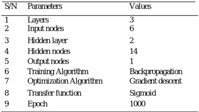
to the neural network. The dataset was parti-tioned into train set, validation set and test set in the ratio of 65:20:15. Table 1 summa-rized other parameters that were set before the commencement of the training.

Table 1: GFFNN Model Design Paradigms

S/N Parameters Values

1 Layers 3

2 Input nodes 6

3 Hidden layer 2

4 Hidden nodes 14

5 Output nodes 1

6 Training Algorithm Backpropagation

7 Optimization Algorithm Gradient descent

8 Transfer function Sigmoid

9 Epoch 1000

Source: Experimentally generated values, Aug., 2014

The proposed GFFNN model used a gradient descent training algorithm which adjusts the weights to move down the steepest slope of the error surface as shown in Table 1. Ac-cording to the information on the same table, the training of the GFFNN is set to terminate at iteration equals 1000 epoch. The objective of training is to minimize the mean square error defined in equation (1) as follows:

where is the simulated output by the GFFNN, and is the target or actual val-ues and E is MSE. The momentum term determines how past weight changes affect current changes. The modified BP training rule is defined as

where η is the momentum term called learning rate, wjk is the weight; and E is the

error parameter. The detail gradient descent algorithm for training GFFNN is presented in the next section.

IMPLEMENTATION

The implementation of GFFNN is carried out on MATLAB 7.6.0 (2008a) platform.

Since the research also intends to compare the accuracy of GFFNN with linear regres-sion (LR) and autoregresregres-sion (AR), the same datasets were used to construct the models for the two statistical tools as well. The re-sults from the implementations are presented in the subsequent section. Fig.1 shows the block diagram of the proposed GFFNN.

I n p u t

s b{1}

LW{2,1}

b{2}

LW {3,1}

b{3}

O u t p u t LW {{}

Input layer Hidden layers Output layer Fig.1: Block Diagram of GFFNN

Where LW is the sum of synaptic weight of all nodes in the input layer, b{1} is the bias of input layer; LW{2,1} is the sum of syn-aptic weight of all nodes in the hidden layer, b{2} is the bias of the hidden node, LW {3,1} is the sum of synaptic weight of all nodes in the output layer and b{3} is the output layer bias.

The most common errors function mini-mized in neural networks are the sum of square errors (SSE) and mean square error (MSE). In this study, MSE was calculated because it shows the average square error between the actual values and predicted val-ues from the network. When MSE is found to be much smaller than 1, the predictive model is found to be reasonable. Other per-formance evaluation criterion used is mean absolute percent error (MAPE).

GRADIENT DESCENT ALGRITHM

Input vectors are applied to the network and calculated gradients at each training sample are added to determine the change in weights and biases. Traingda, an adaptive learning rate function which update the neural network weight and bias values according to the Gra-dient Descent Optimization, was used for the training of the GFFNN. The network is created using newff. The newff creates gen-eralized feed-forward back-propagation net-work with the following syntax:

Syntax:

net = newff (PR,[S1,S2,…..Sn]

{TF1,TF2…….TFn}, BTF, BLF,PF) newff takes several arguments.

PR = R x 2 matrix of min and max values for R input elements

S1 = size of ith layer, for N1 layer

TF1 = Transfer function of first layer (tansig)

TF2 = Transfer function of second layer (log sig)

TF3 = Transfer function of third layer (purelin)

BTF = Back propagation network training function (traingda)

BLF = (Back propagation weigh/bias learning function (learngdm) and returns N – layer general-ized feed-forward back-propagation network.

The connection of the input to the first hid-den layer, second hidhid-den layer and then to output layer is automatically achieved when

newff function is called. And as each layer

has its own transfer function, the newff pro-vides a means of specifying the transfer function of the layers in its syntax. The five parameters associated with traingda are ep-ochs, show goal, time, min-grad, max-fail. The neural network uses the tansig and log-sig for the first and second hidden layers. The aim of using these is to get outputs in those two hidden layers of values between -1 and -1. But since the target values the GFFNN is created to approximate values greater than the range of values between -1 and 1. Purelin is used at the output layer. This enables the network to output values of any magnitude.

A Simplified Algorithm for Training Generalized Feed-Forward Neural Network for Student Enrollment Prediction

Below is a simplified algorithm for training the proposed neural network model for population prediction:

Assemble the training data

1. Initialize the weights that connect inputs to hidden layer 1

2. Multiply the input vectors with their con-necting weights

3. Compute the total weighted input 4. Threshold the total weighted input by

tan-sig to get output for the first hidden layer

5. Use the output for the first hidden layer as the input for second hidden layer.

6. Initialized the weights that connect hidden

layer 1 to hidden layer 2 7. Repeat step 2 and 3

8. Threshold the total weighted input by

log-sig to get output and input for second

hid-den layer and output layer respectively 9. Initialize the weights that connect hidden

layer 2 to output layer

10. Repeat step 2 and 3 to get the output values 11. Threshold the total weighted output by

purelin to get the actual output values

12. If the output values are equivalent to the target values then Goto Stop Else

13. Compute ∑A // ∑A is the difference

between the actual values and the target values.

14. Convert ∑A to ∑I// ∑I is the rate at

which error changes as the total input re-ceived by a unit is changed.

15. Compute ∑W // ∑W is the error

deriva-tives of the weights. That is how the error changes as each weight is increased.

16. Multiply those ∑As of those output units

and add the products

17. Compute ∑As for other layers by repeating

step 12 to 15 moving from layer to layer in a direction opposite the way activities to propagate.

18. Repeat 12 and 13. 19. Stop

20. End

RESULTS AND DISCUSSION

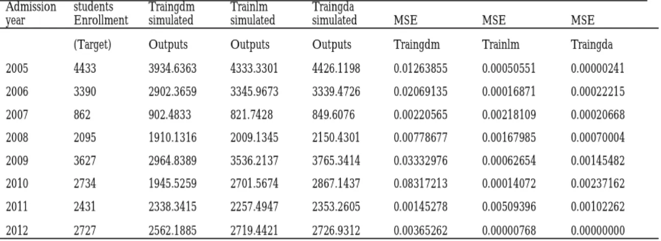
Though the focus of this research is the use of Traindga other training functions: Traingdm (gradient descent with momentum) and

Trainlm (Levenberg Marquardt) were also

used in the experiment as a test on the reli-ability of Traingda. The results are shown in Table 2.

From the results in Table 2, one can infer that Traingda produced the best result and hence suitable for the training of GFFNN. Also from the plots in Fig.2, 3 and 4, it can be observed that Traingda enable GFFNN to minimize mean square errors efficiently

that the other two functions that were used to check its consistencies. According to these figures, the blue plot shows how well the training functions minimize the MSE with the best performance from Traingda.

Table 2: Determining the best training function for GFFNN

Admission year

students Enrollment

Traingdm simulated

Trainlm simulated

Traingda

simulated MSE MSE MSE

(Target) Outputs Outputs Outputs Traingdm Trainlm Traingda 2005 4433 3934.6363 4333.3301 4426.1198 0.01263855 0.00050551 0.00000241 2006 3390 2902.3659 3345.9673 3339.4726 0.02069135 0.00016871 0.00022215 2007 862 902.4833 821.7428 849.6076 0.00220565 0.00218109 0.00020668 2008 2095 1910.1316 2009.1345 2150.4301 0.00778677 0.00167985 0.00070004 2009 3627 2964.8389 3536.2137 3765.3414 0.03332976 0.00062654 0.00145482 2010 2734 1945.5259 2701.5674 2867.1437 0.08317213 0.00014072 0.00237162 2011 2431 2338.3415 2257.4947 2353.2605 0.00145278 0.00509396 0.00102262 2012 2727 2562.1885 2719.4421 2726.9312 0.00365262 0.00000768 0.00000000

Source: Experimentally generated values, Aug., 2014

ANALYSIS OF PREDICTED

RESULTS ON COLLEGIATE

BASIS

Immediately after the training phase, the best function for the proposed model was determined and its performance was com-pared with the selected statistical

ap-proaches: Linear Regression (LR) and Auto-regression (AR), these were done on colle-giate basis for simplicity and ease of

colla-tion. Measures for evaluating the perform-ance of these models are based on the mean absolute percent error (MAPE) defined in equation (3):

(3)

Fig.3: Trainlm function

Linear Regression (LR) model uses linear analysis. Total enrollment, performance in Post-UTME, university budget, tuition fees and student personal security are factors that have impact on enrollment. Total en-rollment was linearly regressed on the school ages 16-35, school budget, and tui-tion fees.

Autoregression (AR) model uses the same variables as the first model, that is, total en-rollment was autoregressed on the appli-cants’ population of ages 16-35, perform-ance in the Post-UTME, school budget, tuition fee and personal security, using 0.5 as the rho parameter (ρ = 0.5). The differ-ence between the second and the first methods is that the second method weights the data of more recent years more heavily than the previous years; while the first method gives the same weight to the data of each year.

After all the necessary computations, the comparison of these models with the pro-posed model is done on the college basis. There are four colleges in the case study used: College of Applied Education and Vocational Technology (COAEVOT), Col-lege of Humanity (COHUM), ColCol-lege of Science and Information Technology (COSIT) and College of Social and Manage-ment Science (COSMAS). Fig.5 shows the results simulated by GFFNN and the two models that were compared with it for COAEVOT. From the figure, it can be ob-served that the performance of GFFNN is better than those of LR and AR. GFFNN only showed poor performance in year 2010 with actual enrollment of 591students and the predicted value of 589 students. On the general note, GFFNN predicts students’ enrollment number for College with a high accuracy. Clearly from fig.6, the

perform-ance of GFFNN is poor only in 2006 when compared with the actual enrollment with value of 409.0 instead of 509 students. The two other models performed quite well here as observed from the graph. The overall re-mark is that the GFFNN performs well in predicting students’ enrollment number in the College of Humanity as shown by Fig.6. The results simulated for COSIT is pre-sented in Fig.7. According to the figure, GFFNN and linear regression performed better than autoregression with the best per-formance on the side of GFFNN, as shown from the graph. Finally, from fig.8, which shows the results simulated by the models for COSMAS, it can be observed that this college admitted the largest number of un-dergraduates hence, remains the most popu-lated college in the University. On the over-all, the performance of GFFNN is very com-parable with the actual enrollment values unlike LR and AR models. From analysis of the results simulated by the models for dif-ferent colleges of the case study, it can be concluded that ANN trained with traingda function provides the better model for the time series of students’ enrollment in tertiary institutions.

PERFORMANCE EVALUATION

OF MODELS

The students’ enrollment trend by different colleges of the University was studied taken into consideration the growth and develop-ment of the school coupled with the recent reduction of tuition fees by the state govern-ment. The result was then used to extrapo-late and predict the students’ enrollment for 2015. The results simulated by the models were computed and evaluated on the basis of Mean Absolute Percentage Errors (MAPE) defined in equation (3) and results are pre-sented in Table 3.

Fig.5: Comparison of GFFNN results with other models (COAEVOT)

Fig.7: Comparison of ANN results with other models (COSIT)

From the above table, MAPE value for lin-ear regression ranges from 0.0254% to 0.0879% with an average of 0.0570%; while for autoregression 0.0184% to 0.1415% with an average of 0.0725% and for GFFNN from 0.0008% to 0.0262% with an average of 0.0101% implying that GFFNN generated the least mean absolute percent errors. Therefore, its simulated results is reliable than the selected statistical ap-proaches used.

CONCLUSION

From the various tests performed on the results of the train, validation and test re-sults in the previous sections, it is con-firmed that Artificial Neural Network per-forms quiet impressive at estimating the students’ enrollment figures. Analysis of the experimental results shows that MAPE value of ANN model ranges from 0.0008% to 0.0262% with an average of 0.0101%, far better than the two statistical models that were compared with it. The MAPE values of LR ranges from 0.0254% to 0.0879% with an average of 0.0570% and that of AR ranges from 0.0184% to 0.0254% with an average of 0.0725%. Hopefully, as the method is adopted in educational matter, the accrued benefit of the model is that, it will help the school management plan

ade-quately for the future needs of the learners in provision of facilities. Also, government, public and private sectors will make reliable and enduring plans that will benefit both the planners and the beneficiaries. The said benefits will also result into more profitabil-ity and improvement in the standard of liv-ing for all and sundry. Further research can be geared towards the use of another Artifi-cial Intelligence approach for the same task.

REFERENCES

Academic Planning and Quality Control Unit, 2013. Students Statistical Reports and

Information, Tai Solarin University of

Educa-tion, Ijagun, Ijebu-Ode, Ogun State.

Bandyopadhyay, B., Chattopadhyay, S., 2008. An Artificial Neural Net approach to

Forecast

the Population of India, 1/9 Dover Place,

Kol-kata-700 019, West Bengal, Idian. E-mail:

[email protected]

Boon M.E, Kok L.P., 1995. Classification

of cells in cervical smears, In Applications rule of Neural Networks, Murray Af, ed. Klawer. pp. 113-131.

Folorunso, O., Akinwale, A.T., Asiribo,

Table 3: Performance Evaluation of Models in Predicting 2015 Enrollment

COLLEGE

Target Value

Predicted (LR)

Predicted (AR)

Predicted GFFNN

MAPE of LR (%)

MAPE of AR (%)

MAPE of GFFNN (%)

COAEVOT 1270 1341.2 1293.4 1262.4 0.0561 0.0184 0.0060

COHUM 967 1023.7 1103.8 992.3 0.0586 0.1415 0.0262

COSIT 1178 1281.5 1299.1 1177.1 0.0879 0.1028 0.0008

COSMAS 2186 2241.6 2245.3 2169.7 0.0254 0.0271 0.0075

Average 0.0570 0.0725 0.0101

O.E., Adeyemo, T.A., 2010. Population

Prediction Using Artificial Neural Network.

Africa Journal of Mathematics and Computer Sci-ence Research, Vol.3(8).pp.155-162.

Guo, S., 2002. Three Enrollment

Forecast-ing Models: Issues in Enrollment Projection for Community Colleges. Presented at the 40th

RP Conference, May 1-3 2002, Asilomar Confer-ence Grounds, Pacific Grove, California.

Guo, S., Zhai, M. 2000. Using Excel and

Visual Basic to Automate Enrollment Pro-jection Processes. The 40th _{Forum of the}

Asso-ciation of Institutional Research, 2000,

Cincin-nati, OH.

Kaastra, I., Boyd, M., 1996. Designing a Neural Network for Forecasting Financial and Economic Time Series. Neurocomputing

(10), ELSEVIER,. pp.215-236.

Keilman, N., Pham, D.Q., Hetland, A., 2002. Why Population Forecasts should be

probabilistic-illustrated by the case of Nor-way. Demographic Research 6(15): 409-453.

Maqsood, I., Muhammad, R.K.,

Abra-ham, A.A., 2002. Neurocomputing-Based

Canadian Weather Analysis, Computational

Intelligence and Applications, Dynamic Publishers Inc., USA: 39-44.

Mehta, A.C., 2004. Projections of

Popula-tion, Enrolment and Teachers. Module on enrollment and populations, National Institute

of Educational Planning and Administration, 17-B, Sri Aurobindo Marg, New Delhi-110016

(INDIA), January 18, 2004.

Mehta, A.C., 1994. Enrolment Projections:

Education for All in India, Journal of

Educa-tional Planning and Administration, Volume

VIII, Number 1, January, New Delhi.

Rufai, F.A., 2014. Students’ Enrollment

Prediction Using Generalized Feed-Forward Neural Network. A thesis Submitted in

Fulfill-ment of the requireFulfill-ment for the Degree of Master of Education in the Department of Computer Science,

Tai Solarin University of Education, Ijebu-Ode, Ogun State.

Song, Q., Chissom, B.S., 1993. New

Mod-els for Forecasting Enrollments: Fuzzy Time Series and Neural Network Approaches.