Vol 62, No 3 (2019)

(1)

TECHNICAL UNIVERSITY OF CLUJ-NAPOCA

ACTA TECHNICA NAPOCENSIS

Series: Applied Mathematics, Mechanics and Engineering Vol. 62, Issue III, September, 2019

THE YOUNG MODULUS ESTIMATION BY CORRELATING

FEA AND EMA FOR AN ELECTRIC MOTOR TEST RIG

Ioan-Claudiu COŢOVANU, Iulian LUPEA

Abstract: The Young modulus estimation for the material of an electric motor test rig is under observation in the present paper. Initially, the modulus of elasticity is approximated at a certain value and a numerical modal analysis is conducted on the test rig in order to find its natural mode shapes and their corresponding natural frequencies. Secondly, three uniaxial accelerometers are placed on the test rig in well-defined positions with the goal of measuring the frequency response functions of the part on three different directions. Lastly, the frequency response functions are analyze and successive runs of the modal analysis are conducted for different values of the Young modulus, until the calculated natural frequencies match the ones from experiment, on one side, and the mode shapes are correlated, on the other side.

Keywords: Young modulus, modulus of elasticity, frequency response function, modal analysis, experimental modal analysis.

1. INTRODUCTION

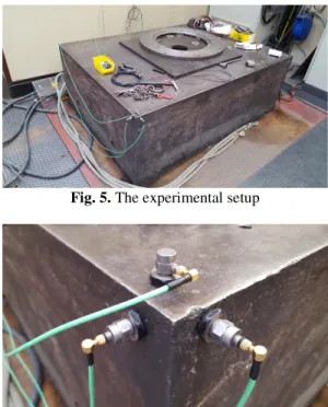
On the occasion of vibration tests and experimental modal analyses conducted on large induction motors, mounted on the cast iron block shaped test rig identified in Fig. 5, a non-negligible influence of the stiffness of the rig was observed, since the dynamic behavior of the tested motors seemed to vary in regards to the mounting position of the motors on the rig, thus suggesting that the rig is not rigid enough to test large machines.

Hence, there is a need to integrate in the numerical simulation models of the tested machines the model of the test rig as well, when correlations of the simulated dynamic behavior of large machines with experimental data, measured while being mounted on the rig, have to be done.

To properly define the dynamic model of the test rig itself, it is necessary to characterize it experimentally by determining the parameters that influence his dynamic behavior. Since its mass would implicitly result by assuming a certain material density value, commonly used

for cast iron, its stiffness remains to be determined, given by the modulus of elasticity.

The Young modulus estimation can be performed by observing the modes of vibration and the associated natural frequencies of vibration. The simplest procedure is by observing the vibration modes when the part is free of constraints [7].

Free vibrations of a structure are rapid conversions between the kinetic and potential energy of it when oscillating about the equilibrium of the structure. During small amplitude vibrations, the Young modulus is the main material characteristic governing the event [7].

(2)

vibration modes. The occurrence of vibration modes is indicated by the shifts in phase, visible on the phase versus frequency graph and associated to magnitude peaks. The phase graph has inflection points at each eigenfrequency, while no shifts in phase are correlated with flat frequency responses (no magnitude peaks).

2. MODAL ANALYSIS OF THE TEST RIG THROUGH FEA

Lacking any CAD data for the test rig, it had to be measured in place. The physical outline dimensions are 1750 x 1250 x 900 mm. Fig. 1 illustrates the 3D model of the rig and the simulation coordinates system, that one will refer to later in Section 3.

Fig. 1. The geometry of the test rig and the simulation coordinates system

The rig is manufactured from cast iron, but the exact type is unknown, therefore there are some assumptions made for the material:

• The density is assumed at 7200 kg/m3_,

giving an approximate mass of 14000 kg for the test rig.

• The Poisson coefficient is assumed at 0.26,

which is a commonly used value for any cast iron.

The mesh elements type and size were properly selecte and a mesh sensitivity study was performed in order to find the optimum model size. Fig. 2, Fig. 3 and Fig. 4 detail the overall mesh grid.

Knowing that the test rig is not rigidly fixed in any way to the ground, but is supported by a sand layer, the modal analysis was conducted with no geometric boundary conditions applied to the simulation model (free vibrations).

Therefore, the boundary conditions are natural, the derivatives of the displacements of the nodes found on the solid’s outer surface being null [2]. Block Lanczos algorithm was used to perform the modes extraction, under the ANSYS Workbench software platform.

The Young modulus of the rig is also assumed at a certain value at first. After the first run, the natural frequencies and the corresponding mode shapes were identified and compared with the experimentally measured ones. New values of the Young modulus were imposed and the modal parameters successively recalculated until they matched the ones determined experimentally, as proposed in [7].

The optimum value for the Young modulus

was finally estimated at 125000 [N/mm2_{]. The}

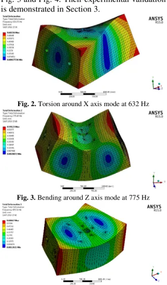
corresponding natural frequencies and the associated mode shapes are revealed in Fig. 2, Fig. 3 and Fig. 4. Their experimental validation is demonstrated in Section 3.

Fig. 2. Torsion around X axis mode at 632 Hz

Fig. 3. Bending around Z axis mode at 775 Hz

(3)

3. EXPERIMENTAL VALIDATION OF THE YOUNG MODULUS THROUGH EMA

The FRF expresses the ratio of the Fourier transformation of the acceleration, velocity or the displacement and the Fourier transformation of the excitation force. More generally, the FRF is the transfer function (TF) between two degrees of freedom of the structure. TF is the ratio between the Laplace transform of the response signal and the Laplace transform of the excitation signal [7].

In the present paper the accelerations are considered, thus the TFs are of inertance type :

( )

2

_{( )}

( )

a

s X s H s

F s

= (1)

where the Laplace transform is applied on the

acceleration _{L x t}_

( )

_=_{s X s}2

( )

&&  and s is the

complex variable [7].

Several different graphical representations of the FRFs are available, among which the Bode diagram, where the magnitude and the phase of the FRF are shown in function of the excitation frequency [7] (Fig. 7, 8, 9, 10, 11, 12, 13, 14).

The following convention is imposed :

• The X axis of the rig is the longitudinal axis;

• The Y axis of the rig is the vertical axis;

• The Z axis of the rig is the transverse axis.

Fig. 5. The experimental setup

Fig. 6. The placement of the accelerometers

3.1. HAMMER IMPACT ALONG X AXIS

As seen in Fig. 7, Fig. 8 and Fig. 9, there are three resonances excited by the hammer impact in the longitudinal direction of the rig.

For the first resonance identified at 634 Hz (Fig. 7), the shifts in phase for the three responses confirm the deformation of the structure in all three directions. There is a more important amplitude for the response of the structure on the Y axis (yellow), lower amplitude on the Z axis (green) and an even smaller amplitude for the response on the X axis (blue). These findings confirm the torsion around X axis mode calculated at 632 Hz.

0 100 200 300 400 500 600 700 800 900 1k [Hz]

2u 5u 10u 20u 50u 100u 200u 500u 1m 2m 5m 10m 20m 50m0.1 -140 -60 20 100 180 [(m/s^2)/N]

Cursor values

X: 634.375 Hz Y(Mg):5.231m (m/s^2)/N Y(Mg):1.814m (m/s^2)/N Y(Mg):3.066m (m/s^2)/N y(Ph):86.294 degrees y(Ph):-37.817 degrees y(Ph):-99.036 degrees

4 Frequency Response H2(Axe Y vertical,Marteau) - Input (Bode Plot - Phase/Magnitude) \ FFT

Frequency Response H2(Axe X longitudinal,Marteau) - Input (Bode Plot - Phase/Magnitude) \ FFT Frequency Response H2(Axe Z transversal,Marteau) - Input (Bode Plot - Phase/Magnitude) \ FFT

Fig. 7. Bode plot – the frequency response functions for the X axis shock, amplitudes around 634 Hz

Next, for the second resonance identified at 771 Hz (Fig. 8), the shifts in phase present for

the three responses also confirm the

deformation of the structure in all three

directions. There are more important

amplitudes for the responses of the structure on the X and Y axis and a considerably lower

amplitude on the Z axis. Therefore,

measurements confirm the bending around Z axis mode calculated at 775 Hz.

0 100 200 300 400 500 600 700 800 900 1k [Hz]

Cursor values

X: 771.250 Hz Y(Mg):5.882m (m/s^2)/N Y(Mg):6.456m (m/s^2)/N Y(Mg):1.472m (m/s^2)/N y(Ph):105.417 degrees y(Ph):-60.660 degrees y(Ph):109.197 degrees

(4)

Finally, for the third resonance identified at 901 Hz (Fig. 9), the shifts in phase present only for the X and Z axis confirm the deformation of the structure in these two directions only and suggest no displacement along Y axis. Also, the amplitudes for the responses on X and Z axis are well distinguished, while the response on the Y axis is flat. All these confirm the bending around Y axis mode calculated at 896 Hz.

0 100 200 300 400 500 600 700 800 900 1k [Hz]

Cursor values

X: 900.625 Hz Y(Mg):1.162m (m/s^2)/N Y(Mg):11.933m (m/s^2)/N Y(Mg):9.107m (m/s^2)/N y(Ph):168.203 degrees y(Ph):-58.739 degrees y(Ph):100.220 degrees

Fig. 9. Bode plot – the frequency response functions for the X axis shock, amplitudes around 901 Hz

3.2. HAMMER IMPACT ALONG Y AXIS

Fig. 10 and Fig. 11 reveal that only the first two resonances are excited by the hammer impact in the vertical direction of the rig.

In the case of the first resonance identified at 633 Hz (Fig. 10), the shifts in phase for the three responses confirm the deformation of the structure in all three directions. There is a more important amplitude for the response on the Y axis, a slightly lower amplitude on the Z axis and an even smaller amplitude for the response on the X axis. These confirm the torsion around X axis mode calculated at 632 Hz.

0 100 200 300 400 500 600 700 800 900 1k [Hz]

Cursor values

X: 633.125 Hz Y(Mg):20.211m (m/s^2)/N Y(Mg):3.782m (m/s^2)/N Y(Mg):12.916m (m/s^2)/N y(Ph):-88.971 degrees y(Ph):96.196 degrees y(Ph):103.667 degrees

Fig. 10. Bode plot – the frequency response functions for the Y axis shock, amplitudes around 633 Hz

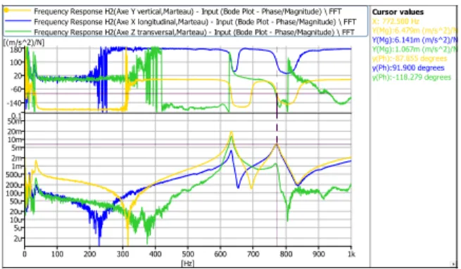
Furthermore, for the second resonance identified at 773 Hz (Fig. 11), the shifts in phase identified for the three responses also confirm the deformation of the structure in all three directions. There are more important amplitudes for the responses of the structure on the X and Y axis and a considerably lower amplitude on the Z axis. Thus, experimental measurements confirm the bending around Z axis mode calculated at 775 Hz.

0 100 200 300 400 500 600 700 800 900 1k [Hz]

2u 5u 10u 20u 50u 100u 200u 500u1m 2m 5m 10m 20m 50m0.1 -140 -60 20 100 180 [(m/s^2)/N]

Cursor values

X: 772.500 Hz Y(Mg):6.479m (m/s^2)/N Y(Mg):6.141m (m/s^2)/N Y(Mg):1.067m (m/s^2)/N y(Ph):-87.855 degrees y(Ph):91.900 degrees y(Ph):-118.279 degrees

Fig. 11. Bode plot – the frequency response functions for the Y axis shock, amplitudes around 773 Hz

Last but not least, one can observ that the excitation along the Y axis (vertical direction) does not excite the bending around Y axis mode, calculated at 896 Hz, since the rig would be moving in the XZ plane only, according to this third mode shape.

3.3. HAMMER IMPACT ALONG Z AXIS

Plots enclosed in Fig. 12, Fig. 13 and Fig. 14 demonstrate that all the three resonances are once again excited by the hammer impact in the transversal direction of the rig.

(5)

0 100 200 300 400 500 600 700 800 900 1k [Hz] 2u 5u 10u 20u 50u 100u 200u 500u1m 2m 5m 10m 20m 50m0.1 -140 -60 20 100 180 [(m/s^2)/N] Cursor values

X: 633.125 Hz Y(Mg):14.568m (m/s^2)/N Y(Mg):2.928m (m/s^2)/N Y(Mg):8.871m (m/s^2)/N y(Ph):94.298 degrees y(Ph):-96.649 degrees y(Ph):-51.626 degrees 4 Frequency Response H2(Axe Y vertical,Marteau) - Input (Bode Plot - Phase/Magnitude) \ FFT

Fig. 12. Bode plot – the frequency response functions for the Z axis shock, amplitudes around 633 Hz

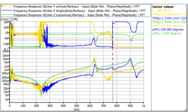
Then, for the second resonance identified at 769 Hz (Fig. 13), the shifts in phase present only for the X and Y axis confirm the deformation of the structure in these directions only and suggest no displacement along Z axis. Also, the amplitudes for the responses on X and Y axis are low, but peaks are present, while the response on the Z axis is flat. These observations confirm the bending around Z axis mode calculated at 775 Hz.

0 100 200 300 400 500 600 700 800 900 1k [Hz] 2u 5u 10u 20u 50u 100u 200u 500u 1m 2m 5m 10m 20m 50m0.1 -140 -60 20 100 180 [(m/s^2)/N] Cursor values

X: 768.750 Hz Y(Mg):623.830u (m/s^2)/N Y(Mg):1.716m (m/s^2)/N Y(Mg):2.783m (m/s^2)/N y(Ph):-87.538 degrees y(Ph):159.485 degrees y(Ph):-7.038 degrees 4 Frequency Response H2(Axe Y vertical,Marteau) - Input (Bode Plot - Phase/Magnitude) \ FFT

Later on, for the third resonance identified at 904 Hz (Fig. 14), the shifts in phase present only for the X and Z axis confirm the deformation of the structure in these directions only and imply no displacement along the Y axis. Moreover, the amplitudes for the responses on the X and Z axis are well differentiated, while the response on the Y axis is flat. These elements confirm the bending around Y axis mode calculated at 896 Hz.

0 100 200 300 400 500 600 700 800 900 1k [Hz] 2u 5u 10u 20u 50u 100u 200u 500u 1m 2m 5m 10m 20m 50m0.1 -140 -60 20 100 180 [(m/s^2)/N] Cursor values

X: 903.750 Hz Y(Mg):1.044m (m/s^2)/N Y(Mg):9.959m (m/s^2)/N Y(Mg):8.242m (m/s^2)/N y(Ph):180.253 degrees y(Ph):83.181 degrees y(Ph):-87.810 degrees 4 Frequency Response H2(Axe Y vertical,Marteau) - Input (Bode Plot - Phase/Magnitude) \ FFT

4. CONCLUSIONS

The results of the numerical modal analysis, i.e. the natural frequencies and the associated mode shapes, as well as their order of appearance, were confirmed by the experimental tests. The correlation of the numerical results with the experimental ones was carried out successfully, within a margin of under ±1%, as data synthesized in Table 1 highlights.

Table 1 Results synthesis Mode Measured frequency [Hz] Calculated frequency [Hz] Difference [%] 1 634 632 -0.3

633 -0.2

2

771

775

+0.5

773 +0.3

769 +0.8

3 901 896 -0.6

904 -0.9

Material properties of the rig to be used in future numerical modal analyses integrating its model as well, are those anticipated in Section 2:

• Density = 7200 [kg/m3_];

• Young modulus = 125000 [N/mm2_];

• Poisson ratio = 0.26.

5. ACKNOWLEDGMENTS

(6)

6. REFERENCES

[1] Brown, D., Allemang, R., Zimmerman, R.,

Mergeay, M., Parameter estimation

techniques for modal analysis, SAE Paper, No. 790221, 1979.

[2] Coţovanu, I. C., Lupea, I., Considerations

on the modal analysis and vibration simulation of induction motors, Acta

Technica Napocensis, Series: Applied

Mathematics, Mechanics and Engineering,

Vol. 62, Issue II, June 2019,pages 351-362.

[3] He, J., Fu, Z.F., Modal analysis,

Butterworth Heineman, Oxford, 2001.

[4] Heylen, W., Lammens, S., Sas P., Modal

Analysis Theory and Testing, Leuven: Katholieke Universiteit Leuven, Department Werktuigkunde, 2007.

[5] Lupea, I., Experimental validation of

acoustic modes for fluid structure coupling in the car habitacle, Proceedings of the

Romanian Academy, Series A –

Mathematics, Physics, Technical Sciences, Information Science, Volume: 18, Issue: 1, Pages: 326-334, Jan-Mar 2017, ISSN: 1454-9069.

[6] Lupea, I., On the modal analysis of a robot,

Proceedings 5th International Workshop on Robotics in Alpe-Adria-Danube Region RAAD '96, pages 309-313, June 10-12 1996, ISBN 963 4204821, Budapest, Hungary.

[7] Lupea, I., The Modulus of Elasticity

Estimation by using FEA and a frequency response function, Acta Technica Napocensis, Series: Applied Mathematics, Mechanics and Engineering, Vol. 57, Issue IV, Nov. 2014, pages 493-496.

[8] Lupea, I., Updating of an exhaust system

model by using test data from EMA, Proceedings of the Romanian Academy, Series A – Mathematics, Physics, Technical Sciences, Information Science, Volume: 14, Issue: 4, Pages: 326-334, Oct-Dec 2013, ISSN: 1454-9069.

[9] Lupea, I., Ciascai, I., Finding vibration

modes for a piezo driven robot structure, Acta Technica Napocensis, Series: Applied Mathematics, Mechanics and Engineering, Vol. 60, Issue III, Sept. 2017, pages 351-357, ISSN: 1221-5872.

[10] Lupea, I., Stremţan, F. A., Topological

optimization of an acoustic panel under periodic load by simulation, Acta Technica Napocensis, Series: Applied Mathematics and Mechanics, Vol. 56, Issue III, Oct. 2013, pages 455-460.

[11] Maia, N. M. M., Modal Analysis,

Experimental | Parameter Extraction Methods, Encyclopedia of Vibration, 2001. [12] Maia, N. M. M., Silva, J. M. M.,

Theoretical and Experimental Modal Analysis, Research Studies Press LTD, 2000.

Estimarea modulului lui Young corelând FEA şi EMA pentru un stand de testare motoare electrice

Rezumat: Estimarea modulului lui Young pentru materialul unui stand de testare motoare electrice este sub

observație în lucrarea de față. Inițial, modulul de elasticitate este aproximat la o anumită valoare și se efectuează o

analiză modală numerică pentru stand pentru a-i identifica formele modurilor sale naturale de vibrație și frecvențele

naturale corespunzătoare. În al doilea rând, trei accelerometre uniaxiale sunt plasate pe standul de testare în poziții

bine definite, cu scopul de a măsura funcțiile de răspuns în frecvență ale piesei pe trei direcții diferite. Funcțiile de

răspuns în frecvență sunt analizate și rulări succesive ale analizei modale sunt efectuate pentru diferite valori ale

modulului lui Young, până când frecvențele naturale calculate corespund celor din experiment, pe de o parte, iar

formele modurilor sunt corelate, pe de altă parte.

Ioan-Claudiu COŢOVANU, Ph.D. Student, Research & Development Manager, NIDEC Oradea

SRL, Cluj-Napoca Working Point, 4 Emerson St., 400641 Cluj-Napoca, _ +40-374-130825,

e-mail: [email protected]

Iulian LUPEA, Professor Ph.D.,Technical University of Cluj-Napoca, Department of Mechanical

Systems Engineering, 103-105 Muncii Blvd., 400641 Cluj-Napoca,  +40-264-401691, e-mail: