Volume 11, Issue 3, September 2014
COMMENTS
ECONOMICS IN PRACTICE
CHARACTER ISSUES
WATCHPAD
Replicability and Pitfalls in the Interpretation of Resampled Data: A Correction and a Randomization Test for Anwar and Fang
Dragan Ilić 250-276
Saying Too Little, Too Late: Public Finance Textbooks and the Excess Burdens of Taxation
Cecil E. Bohanon, John B. Horowitz, and James E. McClure 277-296
Ragnar Frisch and the Postwar Norwegian Economy: A Critical Comment on Sæther and Eriksen
Olav Bjerkholt 297-312
A Reply to Olav Bjerkholt on the Postwar Norwegian Economy
Arild Sæther and Ib E. Eriksen 313-317
Does Occupational Licensing Deserve Our Approval? A Review of Work by Morris Kleiner
Uwe E. Reinhardt 318-325
Capitalism and the Rule of Love
Replicability and Pitfalls in the
Interpretation of Resampled Data:
A Correction and a Randomization
Test for Anwar and Fang
Dragan Ilić
1LINKTO ABSTRACT
In their article “An Alternative Test of Racial Prejudice in Motor Vehicle Searches: Theory and Evidence,” published in theAmerican Economic Reviewin 2006, Shamena Anwar and Hanming Fang (hereafter AF) study motor vehicle stops and searches by Florida Highway Patrol officers (“troopers”). Their data include the race and ethnicity of the trooper as well as of the motorist stopped and possibly searched. A search of a stopped motorist is deemed successful if the trooper finds contraband in the vehicle. Using data on troopers and motorists of three race-ethnicity groups (white non-Hispanic, black, and white Hispanic, with others being dropped), AF compute nine motorist search rates and nine trooper-on-motorist search-success rates. They present a model that exploits this information to test whether troopers go beyond statistical discrimination to racial prejudice.
The model has an implication that would be unaffected by whether troopers exhibit racial prejudice. This implication is testable and concerns the rank-order of the search and search-success rates. AF report that, across the board, the data neatly fit the model’s predicted inverse rank-order implication, strongly supporting the soundness of the model.
AF then apply the model to address the question of racial prejudice. They do not find evidence of racial prejudice; in my own analysis, I, too, do not find
ECON JOURNAL WATCH 11(3) September 2014: 250-276
such evidence. The present critique, then, does not arrive at results about prejudice contrary to their results.
The present critique starts by reporting that I cannot replicate their preliminary inverse rank-order findings. For each of the nine trooper-on-motorist categories, AF report the search rate and search-success rate. However, I find that replication is not possible for two of the nine reported search-success rates. Correspondingly, replication is not possible for the reported statistical significance of four of the sixZ-statistics and one of the threeχ2test statistics for the rankings of the search-success rates. These new results obliterate the reported distinct pattern of the rates and imply that the empirical support for the model’s soundness is not what AF claim it to be. In consequence, our confidence in the results obtained by employing the model to test for racial prejudice should be significantly reduced.
While the problem of irreplicability is my primary point, I then move on to another matter. My replications draw attention to a neglected statistical caveat in AF’s implementation of the empirical tests of racial prejudice. The replications happen to show that the novel resampling procedure employed by AF does not provide robust results. I pinpoint the empirical source of the lack of robustness, and, in an appendix, show how a simple extension to their method improves robustness. In another appendix I put forth an alternative randomization test that seems more appropriate when testing such resampled data.
With all improvements, we still do not find evidence of racial prejudice. But now we know that our knowledge about the issue is poorer than one might have guessed from reading AF.
Recap of Anwar and Fang (2006)
When a highway patrol trooper stops a motorist, he or she faces a decision of whether to search the vehicle. Consider a police force with different trooper racial groups facing motorists classified by the same races. The model postulates that each trooper racial group is characterized by a specific cost of searching motorists. We say that a given trooper racial group is racially prejudiced if their search cost depends on the race of the motorist they search. For example, consider white troopers. Suppose their cost of searching white and black motorists were the same, while their cost of searching Hispanic motorists werelower.2This would be a case
of racial prejudice, although it is unclear whether we would describe the prejudice as one against Hispanic motorists or as one in favor of white and black motorists.3
In addition to the cost of search, a trooper’s decision to conduct a search depends on the likelihood of the stopped motorist being engaged in criminal activity. The trooper infers this probability from an informative but noisy signal emitted by the motorist during a stop. This ‘guilt’ signal captures all possible characteristics linking the motorist to criminal activity. Given the trooper’s search cost, the strength of this signal has to exceed a certain threshold in order for the trooper to expect a benefit from searching.
For every combination of motorist and trooper racial groups, there exist equilibrium search and search-success rates that are both determined by a threshold value of the guilt signal. As a trooper, if I have a high search cost, then I had better expect a motorist to be guilty with a correspondingly high probability before I consider searching him. Because the guilt signal is informative, this implies that the lower the rate at which I search motorists, the higher will be my resulting search-success rate.
To illustrate this inverse relationship in more detail, suppose I am a white trooper and I do not harbor taste-based prejudice. On the postulates of the model, this means that my cost of searching a motorist is the same regardless of whether the motorist is white or black. My cost of searching a white motorist’s car is no higher than my cost of searching a black motorist’s car. Now suppose that I, a white trooper, do harbor taste-based prejudice against blacks. This may be thought of as a search-cost reduction for my searching black motorists, vis-à-vis white motorists. Such a search-cost reduction would lead to a guilt probability threshold for my searching black motorists lower than such threshold for white motorists. In other words, now a lower probability of guilt on the part of a black motorist (in comparison to a white motorist) satisfies the requirements to conduct a search. On the one hand, this raises the search rate towards blacks because now a greater fraction fulfills the search criterion. On the other hand, among that larger fraction, proportionally less are actually guilty than among the searched white motorists.
For a given race of troopers, differing search costs against the different motorist races translates into racial prejudice. But even without racial prejudice, search costs may differin generalbetween the trooper racial groups. That is to say, some trooper racial groups may have equally higher search costs against all motorist racial groups, which does not imply racial prejudice. To put it in AF’s terms of the police force being either “monolithic” and “non-monolithic,” a monolithic police force would not imply that there is no racial prejudice, and a non-monolithic police force would not imply that the police are racially prejudiced. Not only do Anwar
and Fang allow for non-monolithic behavior in contrast to previous models, their model actuallyexploitssuch behavior in order to deliver testable implications about the presence of racial prejudice. Indeed, their model is not instructive if the police are, in fact, monolithic.
To understand how the model construes and infers “prejudice,” consider a police force in which black troopers have higher search costs against white motorists than white troopers do. Assuming no prejudice, it then follows that the search costs of black troopers against black motorists are the same as they are against white motorists. In addition, the search costs of white troopers against black motorists are the same as they are against white motorists. By transitivity, it follows that the search costs of black troopers against black motorists are also higher than the search costs of white troopers against black motorists. Put differently, if not prejudiced, black troopers have generally higher search costs which are not associated with the race of the motorist, and thus the race of the motorist plays no role when ranking the search costs by trooper race. This independence translates to the search and search-success rates. Recall that these rates are monotonically linked to the search costs such that when there is no prejudice, the black troopers’ search rates against any given race of motorists are smaller than the white troopers’ search rates; and the black troopers’ search-success rates against any given race of motorists are larger than the white troopers’ search-success rates.
AF’s test for racial prejudice assesses this predictedrank independence. If the ranking of the search or search-success rates depends on the race of the motorist, then racial prejudice on the part of the police can be deduced. Note that this inference of prejudice is relative because the method cannot determine which trooper racial group(s) is (are) prejudiced. At the same time, this ranking offers a test for the soundness of the model. Regardless of whether racial prejudice exists, this other testable implication predicts that for a given race of motorists, the rank order of the search and the search-success rates should always be exactly the opposite. In the above example, black troopers should always be the ones that are least likely to search against a given motorist group, but if they do, they should always exhibit the highest success. This fundamental implication is called the model’sinverse rank order condition.
In their analysis, AF cannot reject the hypothesis that troopers of different races do not exhibit relative racial prejudice. That is, their data suggest that the rankings of the search and search-success rates by trooper race do not seem to depend on the race of the motorist. What is more, the inverse rank order condition is firmly satisfied in all cases. The reportedZ-statistics from the rank order tests indicate distinct ranks in the predicted manner with high statistical significance (p
rates against any race of motorists, followed by Hispanic troopers. Black troopers are the least likely ones to perform a search. If black troopers search, however, they are the most successful group. In turn, Hispanic troopers have higher search-success rates than white troopers. A perfect fit, the reported pattern of these rank orders lends strong support to the descriptive validity of the model.
The validity of the empirical tests hinges on the assumption that the fraction of motorists of a given race carrying contraband does not depend on the race of the troopers searching them. The raw data, however, indicate that this assumption might not be empirically valid. White, black, and Hispanic troopers are dispersed disproportionately across the eleven regional troops in Florida and thus do not seem to face similar pools of motorists.4 For this reason, the application of the empirical tests implements a clever novelty. AF introduce a sophisticated resampling procedure to create a reweighted data set that meets this assumption and serves as the basis for the empirical tests. To alleviate sampling error, this reweighted data set is the average of 30 independently drawn resamples using the procedure. This makes the search and search-success rates reported in AF the bootstrapped means from the corresponding rates calculated in each of the 30 draws. By the same token, every empirical test in AF is based on the average of the corresponding test statistics calculated in each of the 30 independent resamples.5 In what follows, I refer to the execution of AF’s procedure with 30 iterations as a “pass.”
A few words on
monolithic behavior and semantics
Before we proceed to the replication, a few words are in order for the reader that is unfamiliar to the literature. As noted already, we work with three racial groups: white, black, and Hispanic. The combinations for trooper-on-motorist make nine cells for the search and search-success rates, respectively. The previous section has shown that Anwar and Fang’s model allows for the possibility that the trooper racial groups have different search costs against a given race of motorists, a behavior they dub “non-monolithic.” In the context of such non-monolithic behavior, there is a basic assumption made in modeling trooper behavior, an assumption employed by AF and maintained throughout my own analysis, including my renovations. For the moment, consider only the search-success rate
4. See Figure 1 in AF (2006, 142) for the troop locations.
cells.6The modeling postulates, for example, that in the cell for Hispanic troopers searching white motorists, the cost of searching is the same for all troopers within that cell. That is, the postulate says that the cost to a Hispanic trooper of searching the car of a white motorist is the same, irrespective of which Hispanic trooper it is and which white motorist it is. The term non-monolithic is apt in that we have nine different combinations and the cost of search is allowed to differ among them, a generalization that sets AF’s model apart from previous ones. But the term is a little misleading becausewithin each of the nine cellsthe search-cost assumption is in fact monolithic. Put differently, there is heterogeneity across the nine cells, but homogeneity within each of them.
The reexamination shows that the data, in fact, should make us uncom-fortable about the postulate of homogeneity within each cell.7 But that is a weakness of my own analysis as well as AF’s. It is, as it were, yet another reason to figure we do not really know what we seek to know (that is, whether racial prejudice plays a significant role in trooper behavior).8
The reader should also be alerted to the very distinct way of construing and modeling “prejudice” in this branch of the literature. I follow the semantic practice of AF and the preceding literature in talking of prejudice; see, for example, the seminal work by John Knowles, Nicola Persico, and Petra Todd (2001). In our semantics, prejudice is said to be present when troopers of a given race have search costs that depend on the race of the motorist. More precisely, a trooper is deemed prejudicedagainst group X if the search costs against a motorist of group X are lower than they are against a motorist of group Y.9With this approach of modeling prejudice, a biased trooper requires a lower guilt signal on the part of a group X
6. The same reasoning applies to the search rate cells. More precisely, in what follows we are talking about the nine trooper-on-motorist search cost combinations, which uniquely determine both the search and the search-success rate combinations.
7. In Ilić (2013, 50ff.), I elaborate on this issue of heterogeneity in the police force.
8. The issue of homogeneity vs. heterogeneity also crops up in other dimensions. In another paper I show that aggregating police stop and search data across time and regions involves the danger of false conclusions when testing for racial prejudice with the established economic models (Ilić 2013). For example, when singling out troop G in AF’s data, we cannot reject prejudice using AF’s framework, a conclusion that drowns in their aggregate analysis. What is more, in troop C, the region with the largest number of searches, the inverse rank order condition predicted by AF’s model is violated with statistical significance, a violation that refutes the model for these data. The same holds true for troops E and K. These violations are lost in the aggregate analysis, yet these three troops account for half the searches in the aggregate data.
motorist in order to trigger a search. One could also argue that the trooper draws utility from disadvantaging a motorist of group X by means of searching them. Yet by the same token, one could argue that the trooper is prejudicedin favor ofgroup Y because the trooper cuts even relatively suspicious group Y motorists some slack, or because the trooper would draw disutility from annoying a group Y motorist.10
Although the idea of favoring a group is mentioned in the early literature, it comes up only in connection with favoring black motorists from fear of future litigation when searching them (Knowles, Persico, and Todd 2001, 227).11 The notion of actively favoring in terms of sympathy only emerged with additional empirical information on trooper race (Close and Mason 2007). Favoring is not explicitly brought up in AF. The problem with favoring is that it would undo a researcher convention of the anchoring of treatment. As described in the above example, it might well be that a trooper is not prejudiced against motorists of group X despite the lower search costs. This is the case if these search costs actually reflect theunbiased benchmark. The trooper might simply favor group Y, and that is all there is to it. This semantic difference has consequences for the interpretation of the data in AF’s framework. If the observed rank orders are not consistent with the hypothesis of no relative racial prejudice, then one cannot readily say whether these results imply the presence of malevolent prejudice or preferential prejudice. All one can deduce is that there is something racially non-neutral in police behavior. So when AF stress that their model can only detect relative racial prejudice (because one cannot say which trooper race(s) are biased), it should also be clarified that furthermore, the model cannot distinguish between favoritism and animus if it detects prejudice. This bears importance for policy recommendations.
Replication
The meaning of replication requires some clarification. Because the reported search and average search-success rates are calculated via AF’s novel resampling procedure, they are stochastic and vary to some extent in each iteration and thus from pass to pass. The same reasoning applies to the test statistics. An exact replication of AF’s results is therefore unlikely. To account for the stochastic leeway in the replication, I have automated AF’s tedious task of manually proces-sing the 30 iterations that make up one pass and have conducted 10,000 independent passes. In other words, I have calculated essentially all the possible results that the resampling procedure can produce with AF’s data.12
The replications expose two problems in AF’s paper. First, two of the nine reported average search-success rates cannot be replicated in that they do not fall within the domain of possible outcomes. Second, in the same vein, four of the six
Z-statistics used in the rank order tests and one of the threeχ2test statistics used in the preceding test of monolithic trooper behavior cannot be replicated. As a consequence, these test statistics no longer reject the respective null hypotheses of equal rates.13Taken together, these two issues negate the empirical support for the model.
Consider first the replication of the nine estimated average search-success rates, which, in AF, are reported in Panel B of their Table 1 (2006, 130). The frequency distributions that I obtained by the automated replications of the rates using the resampling procedure are shown in Figure 1. For ease of comparison, the arrangement is in line with the combinations of motorist and trooper racial groups in AF’s Table 1. That is, the left, the middle, and the right column depict white, black, and Hispanic troopers, respectively. In turn, white, black, and Hispanic motorists are arranged by upper, middle, and lower row, respectively. So for instance, the upper left distribution shows that the bulk of the 10,000
indepen-12. The 10,000 automated replications are calculated using AF’s original Stata resampling algorithm and employ their data, both of which are available at theAmerican Economic Reviewwebsite. I have used Stata version 13 and, for a previous draft, version 11. In keeping with AF’s code, no specific seed was set prior to the resampling. Setting specific seeds or using truly random seeds via the Stata packagesetrngseeddid not affect the general results from the replication. Appendix 3 links to an online resource that provides a more detailed description of my replications including additional data, codes, and figures. Among these additional data are the frequency distributions of the replicated search rates, which do not show any deviation from AF’s reported values and are thus omitted from the discussion in this paper.
dently estimated average search-success rates of white troopers against white motorists falls between 24 and 25 percent. This is consistent with AF’s particular pass that yielded 24.3 percent, indicated by the vertical red line: These lines in Figure 1 are AF’s reported estimates of the average search-success rates.
Two of the nine reported rates (the red lines) cannot be replicated in this way. Figure 1 shows that AF’s estimated average search-success rates of Hispanic troopers against black and Hispanic motorists, respectively, fall outside the com-puted ranges: In contrast to the reported 20.8 percent, the replications place the possible average search-success rates of Hispanic troopers against black motorists between 17 and 19 percent. And against Hispanic motorists, the possible rates of Hispanic troopers range from 21 to 28 percent. At 14.3 percent, the reported value lies below this spread.14Put differently, these two reported rates cannot be squared with the data even when accounting for the variation in possible outcomes.
In contrast to the reported pattern in AF, the replications of the average search-success rates displayed in Figure 1 no longer provide empirical support for the inverse rank order condition predicted by the model. Recall that the pattern of the search rates in the data predicts that, against any given race of motorists, black troopers should search with the most success, followed by Hispanic troopers. White troopers should display the lowest average search-success rates. AF’s values, indicated by the red lines in Figure 1, fit this prediction perfectly. Both the two irreproducible rates, however, run afoul of this prediction. On the one hand, the replications disclose that Hispanic troopers are the least successful ones when it comes to searching black motorists. On the other hand, the replications also reveal that they are the most successful trooper group against Hispanic motorists. At first glance, this seems to have severe consequences for the model. Given the scale of theZ-statistics associated with the relatively small differences in means reported in AF (p. 146), the new rates would not only revoke the empirical support for the model. They would actually violate the inverse rank order condition with high statistical significance and would thus formally refute the model (p. 138).
Figure 1. Frequency distributions of replicated average search-success rates
This takes us to the second issue with respect to irreproducibility. The empirical tests reported in AF support all predicted rank orders with high statistical significance. For example, AF test whether the difference in the average search-success rates of white and Hispanic troopers against white motorists (24.3 and 26 percent, respectively) is different from zero. They report a Z-statistic of −324.1, making a clear case for a distinct rank order. The other reportedZ-statistics are in the same ballpark.15My replications, however, show that the data cannot account for these magnitudes. On the contrary, most rank orders of the average search-success rates turn out not to be statistically significant, a result that also happens
to render the aforementioned violation of the inverse rank order condition merely descriptive.16
Figure 2. Frequency distributions of replicatedZ-statistics from AF’s pairwise differences in means tests of search-success rates by trooper race for a given race of motorists (null hypothesis: no difference)
Figure 2 depicts the frequency distributions of all replicatedZ-statistics from the pairwise rank order tests of the average search-success rates, again based on 10,000 passes. The first two columns replicate AF’s six rank order tests for the average search-success rates against white, black, and Hispanic motorists, respec-tively, which are listed by row. The first column tests whether the difference of the average search-success rates between white and Hispanic troopers is zero. The second column does the same for Hispanic and black troopers. As additional
evidence to AF’s tested rank orders, the third column tests the difference between AF’s first and third rank, that is to say, black and white troopers. Despite the spreads, each distribution of possible Z-statistics in Figure 2 paints an unam-biguous picture in terms of statistical significance when considering conventional significance levels.17 The outcomes show that the statistical significance of four of the six reported rank order tests for the average search-success rates cannot be replicated. For instance, in contrast to the aforementioned Z-statistic of −324.1 when testing the difference in the average search-success rates of white and Hispanic troopers against white motorists, the upper left distribution indicates possible outcomes between −0.9 and zero, values that cannot reject the null hypothesis of equal rates.18Two of the six rank orders remain consistent with the reported statistical significance in AF, albeit at lower levels. First, the difference in the average search-success rates of black and Hispanic troopers against white motorists. And second, as a coincidental consequence owing to the new value of the replicated average search-success rate depicted in the lower right distribution in Figure 1, the difference in the rates of white and Hispanic troopers against Hispanic motorists becomes statistically significant. In contrast, AF’s value at 14.3 percent would not have rejected the null.19
Finally (not depicted), one of the threeχ2test statistics from AF’s test of monolithic trooper behavior with respect to the average search-success rates cannot be replicated. This test precedes the rank order tests and, in showing that the trooper racial groups exhibit a distinctive stop and search behavior on the whole, lays the foundation for the application of the rank order tests. At the same time, it highlights the model’s advantage in comparison to the seminal framework by Knowles, Persico, and Todd (2001). When testing for monolithic behavior against black motorists, Table 1 in AF indicates a p-value of <0.001, rejecting the notion that the troopers behave differently against black motorists. Yet the replicated frequencies of successful and unsuccessful searches based on 10,000
17. Except for maybe the lower right corner, which depicts the frequency distribution of theZ-statistic for the difference of the average search-success rates between white and black troopers against Hispanic motorists: four of the 10,000 passes yield an averageZ-statistic above −1.64 and would thus fail to reject the null hypothesis at the five percent level.
18. Thisp-value from the replication corresponds to results reported in Knowles, Persico, and Todd (2001), who test for similar differences in search-success rates with a comparable sample size. For example, when testing for the difference in the rates against black motorists (34 percent in 1,007 searches) and white motorists (32 percent in 466 searches), they cannot reject a difference of zero (by means of aχ2test). In
comparison, using the resampled sample size from a random iteration, I cannot reject that the difference between the rates of white (24.6 percent in 1,846 searches) and Hispanic troopers (23.2 percent in 211 searches) against white motorists is zero.
passes yield possibleχ2values between 1 and 2.5, implying that the three average search-success rates against black motorists are not likely different from each other. TheZ-statistics for the rank order tests against black motorists in the second row of Figure 2 support this inference. A back-of-the-envelope calculation shows that this new value of theχ2test statistic is not due to the new average search-success rate estimate of Hispanic troopers against black motorists.
Upon reexamination, then, the data no longer indicate a discernible pattern of the rank orders of the search-success rates. This does not refute the model. The replications do, however, rescind the reported strong empirical support.
But the replications raise yet another issue. The variation among the esti-mated average search-success rates and the estiesti-mated test statistics provided by the resampling procedure gives reason to reconsider the conclusiveness derived from the empirical tests. Does robustness pose a serious problem in AF’s data? Figure 2 shows that despite the spread in the estimated test statistics, the statistical inferences from AF’s data (as measured by conventional significance levels) do not depend on the outcome of the resampling. Figure 1, on the other hand, indicates a slight overlap in the distributions of the estimated average search-success rates of white and Hispanic troopers searching white motorists. So depending on the particular pass, the estimated rates may give even less descriptive support for the inverse rank order condition. But by and large, things do not look bad in AF’s data despite the imprecision of the estimates.
Other data might be less forgiving. The volatility of the estimates opens up the possibility that the same data can give rise to conflicting conclusions. For one, the rank order tests on the basis of the resampling procedure could erratically indicate the presence or absence of racial prejudice. This is primarily a concern if one uses only search data in the empirical tests.20 Because search data have smaller sample sizes than stop data, they are more prone to volatile outcomes via the resampling procedure. Overlaps in the frequency distributions of the possible outcomes could then randomly imply (in-)dependence of the rank order for a given race of motorists, indicating the (absence) presence of racial prejudice. An additional issue arises when using both stop data and search data for additional evidence, such as AF do, i.e., to test the soundness of their model via the inverse rank order condition. When doing so, fickle outcomes might sometimes lend (some) support to the model, only to refute it in another pass by violating the inverse rank order condition with statistical significance. Such caprice is vexing. In Appendix 1, I show that raising the number of iterations is a simple solution to
mitigate the risk of reaching arbitrary conclusions. The next section sheds light on the empirical source of the nonrobustness of the estimates.
Resampling procedure and
disaggregated trooper data
The considerable range of possible outcomes produced by the resampling procedure raises the question of what is triggering the volatility. Toward the answer, this section first describes the resampling procedure in detail. I then look at the trooper search pattern and racial trooper locations in AF at a disaggregated level, which turn out to be the decisive empirical factors that drive the precision of the estimates.21
In each troop, AF’s resampling procedure randomly draws a subsample (without replacement) for each trooper race in relation to their aggregated proportion in the data. As an approximation, AF use proportions of 75, 15, and 10 percent for white, black, and Hispanic troopers, respectively.22 Through the trooper identifier, these subsamples are subsequently merged with the raw stop and search data, forming the sample stop and search data. Put differently, the resampling procedure prescribes a number of draws for each trooper race in each troop and only keeps those observations from the raw stop and search data that are carried out by troopers who were drawn in the resampling. From the sample stop and search data, the aggregate number of stops and (successful) searches are tabulated for each trooper/motorist race combination, yielding the search and search-success rates. These rates are then tested for non-monolithic behavior and for differences in means. To alleviate the sampling error caused by the random draws, AF conduct 30 iterations of independent resamplings, taking the average of the corresponding search and search-success rates and the test statistics from each iteration. The previous section has highlighted that a statistical problem arises in this procedure. Despite averaging over 30 iterations, the values provided by this method fluctuate substantially.23
21. Recall that AF employ the resampling procedure because the raw data indicate that troopers of different races are not randomly assigned to motorists of different races. Depending on the data, the empirical tests may well be applicable without any prior resampling.
22. The exact shares for these groups in the data are 76.3 percent, 13.7 percent, and 10 percent. AF maintain strict multiples of 75/15/10.
TABLE 1. Trooper distribution and sample ratios by troop and race
Panel A: Trooper distribution Panel B: Sample ratios
Trooper race Trooper race
Troop White Black Hispanic Troop White Black Hispanic
A 120 7 2 A 0.125 0.429 1
B 88 8 3 B 0.170 0.375 0.667
C 155 22 13 C 0.581 0.818 0.923
D 176 26 20 D 0.682 0.923 0.800
E 68 39 58 E 0.882 0.308 0.138
F 125 8 9 F 0.240 0.750 0.445
G 105 17 4 G 0.286 0.353 1
H 62 8 0 H - -
-K 81 17 18 K 0.926 0.882 0.556
L 91 45 15 L 0.989 0.400 0.800
Q 41 4 5 Q 0.366 0.750 0.400
One can show that the dispersion is driven by the underlying heterogeneous trooper search behavior. AF’s trooper data set contains information on 1,469 troopers conducting 8,976 searches. In the resampling, the variables of interest are their race and troop assignment. Define the sample ratio as the prescribed number of troopers of a given race in the subsample divided by their actual number in that troop. Panel A in Table 1 tabulates the race/troop allocations in the raw trooper data, which pin down the sample ratios in Panel B.
The variation in the sample ratios captures the differences in the racial composition of troopers between the troops. In each troop, the most underrepresented trooper race sets the bar for the sample ratios of the other racial groups. Consequently, troops that are disproportionate in comparison to the racial proportion of the entire police force induce lower sample ratios.24For example, because of the relative Hispanic dominance in troop E, a Hispanic trooper only has a 13.8 percent chance of being selected into the subsample. On the other hand, the presence of merely two Hispanic troopers in troop A severely limits the sample ratio of their white colleagues: While the Hispanic troopers in troop A do not undergo any resampling, a white trooper is drawn with a probability of 12.5 percent. Troop H illustrates the extreme case of disproportion. Its lack of Hispanic
troopers leads to the omission of the entire troop in the resampling procedure, discarding its share of observations in the data.25
In addition to the racial disproportion between troops, the trooper data reveal a striking imbalance in the number of searches at the individual level. It turns out that 742 of the 1,469 troopers never search and drop out when merging the trooper subsamples from the resampling procedure with the raw search data. Of the troopers actually contributing to the aggregated search data, 727 conduct at least one search, 530 at least two, and 431 at least three searches. When considering only troopers with more than ten searches, 194 remain. The dots in Figure 3 visualize this heterogeneous search behavior. Each dot represents one of the 727 troopers that has conducted at least one search. The x-axis denotes the number of searches per trooper and the left y-axis measures their cumulative distribution. The skew highlights that most troopers rarely search, but a few do so vigorously.26
Figure 3 also incorporates data on individual search-success rates associated with the total number of searches conducted by each trooper. Measured on the right y-axis, each plus represents a trooper’s search-success rate that corresponds to her dot on the same latitude. Crucially, the data suggest a negative relationship between the number of searches and the search-success rates, a finding which is independent of trooper race. In general, the more searches a trooper conducts, the smaller the overall chance is of uncovering engagement in criminal activity. This relationship affects the precision of the estimates provided by the resampling procedure because, for any troop, the draws within the racial groups give each trooper the same probability of becoming part of the subsample without consideration of her particular search-success rate and, more importantly, her number of searches. On a different note, the negative relationship between the
25. There are two ways to increase the sample ratios. I was able to obtain an updated trooper data set from the Florida Highway Patrol, which contains information on 122 additional troopers covering the same time frame. The new data improve the racial balance in disproportionate troops, doubling most sample ratios. Moreover, troop H can be kept in the resampling procedure due to the presence of six Hispanic troopers. Alternatively, starting from the most underrepresented group, the numbers drawn in the resampling for the other groups could be rounded to the nearest integers in relation to their overall proportion. Depending on the troop and trooper race, the probability of being selected into the subsample could accordingly be increased by almost 50 percent. As in AF, the empirically testable model assumption that the troopers face the same pool of motorists determines the applicability of this and other alternative ways to increase the sample ratios. Nevertheless, neither the new data nor the laxer proportion requirement change any of the conclusions in this paper. I would like to thank John Knox and Richard Taylor from the Florida Highway Patrol for their support in obtaining the additional data.
number of searches and the search-success rates qualifies the model assumption of monolithic behavior within any given racial trooper/motorist group combination.
Figure 3. Trooper heterogeneity in searches and search-success rates
As an illustrative example of how this relationship affects the precision of the estimates, consider a troop with three troopers of raceX. Let trooperx1conduct 99 searches, 33 of which are successful. Troopers x2and x3 each conduct three searches, two of which are successful. Trooperx1searches much more often than
x2orx3but, relatively, does so with less success. Let the sample ratio be⅔ and draw the corresponding subsamples. The aggregated search-success rates for the three possible subsamples are 34.31 percent, 34.31 percent, and 66.66 percent. With independent resampling, the average search-success rate converges to 45.10 percent. The inclusion of x1 in a subsample introduces a bias in the aggregated rate towardsx1’s rate and stems from her disproportionate share in the aggregated number of searches. So the spikes in the aggregated search-success rates in the subsamples are caused by trooperx1.
decrease of precision in the estimated rates. Figure 3 gives an idea of the impact a single trooper can exert on the average search-success rates.27The extent of the instability such troopers can evoke in the resampling depends on their probability of becoming part of their subsample. The lower the sample ratio, the lower is the probability of a trooper being selected. In practice, this depends on the empirical distribution in trooper race across troops, as seen in Table 1.
The selection probability also depends on the proportion of non-searching troopers. The data show that only every other trooper ever conducts searches. Accordingly, among the subsample of drawn troopers, only a fraction provides actual data for the calculation of the search-success rates. For example, of the 39 black troopers in troop E, 12 find their way into the subsample. Yet out of these 39 troopers, as few as eight conduct searches. In a random draw, it is unlikely for them to be selected simultaneously into the subsample of 12. One can show that most likely, the subsample will only include one, two, three, or four searching troopers (with probabilities of 0.17, 0.32, 0.29, and 0.14, respectively). Thus in addition to the sample ratio, non-searching troopers further limit the presence of searching troopers in the subsamples, amplifying the fluctuations of the estimates provided by the resampling procedure.
To sum up, the interaction of non-searching troopers, the sample ratios, and the negative relationship between the number of searches and the search-success rates decreases the precision of the estimates and explains the large ranges of possible outcomes provided by the resampling procedure displayed in Figure 1 and 2. Appendix 1 shows that raising the number of iterations is an obvious and easily implementable solution to enhance the precision of the estimates, mitigating the risk of pass dependence in general and, in turn, lowering the risk of false conclusions from the data.
Conclusion
The replications in this paper do not bear out the empirical results reported in Anwar and Fang (2006). In contrast to the predicted inverse rank orders of the
search-success rates which are firmly buttressed by the empirical tests conducted in AF, the data no longer reveal that distinct pattern and therefore do not provide empirical support for the model. That does not take away from AF’s theoretical contribution. It does point out, however, that the data do not nearly fit their model as well as previously thought. In this sense, AF’s main empirical conclusion that the police do not exhibit racial prejudice stands on less firm ground.
This paper also draws attention to a neglected statistical problem that affects the interpretation of the empirical results. Because the data do not seem to satisfy a crucial condition of the model, AF make use of a novel resampling procedure to create a reweighted data set. It turns out that the estimates provided by this procedure lack precision. Although AF’s replicable results are only affected quali-tatively, the imprecision creates a non-negligible risk of severely misinterpreting other resampled data. Depending on the outcome of the resampling, one might infer racial prejudice when there is none (or vice versa). And more fundamentally, one might support or reject the model when there is no reason to do so. Resampling with 30 iterations as conducted by AF seems too few to yield conclusive estimates.
In Appendix 1, I show how simply raising the number of iterations improves robustness. There is no general rule how many iterations are needed for conclusive results, but the existing bootstrap literature suggests that 1,000 replicates should suffice. On another note, it is not obvious that the parametric tests employed in AF are appropriate to test the complex data obtained by the resampling procedure. To inform future research further, Appendix 2 presents a randomization test that provides an alternative and more expedient way to empirically test the observed rank orders. A randomization test seems more appropriate than conventional statistical tests for it makes no assumptions about the distribution of the resampled data. In light of today’s computational power, both raising the number of iterations for higher accuracy and randomization no longer pose a problem and can be readily implemented in existing software.
take into account the accuracy of their estimates before interpreting any resampled data.
More conclusiveness is clearly desirable to mitigate the neglected risk of jumping to false conclusions, such as when assessing racial prejudice among a police force. But the robustness has yet another merit. It prevents malicious cherry-picking of a particular outcome that suits a given agenda. Suppose biased re-searchers are aware that the possible outcomes of the resampled data support two diametrically opposed interpretations. In that case, they might deliberately report the convenient but wrong interpretation, an interpretation which is replicable at that and which, for this very reason, would leave them unscathed.
Summary of appendices
There are three appendices. The first appendix presents a straightforward and easily implementable solution to enhance the precision of the estimates provided by AF’s resampling procedure. The second appendix puts forth a randomization test and argues that it is a more expedient way to test differences of average rates in a resampling. The third appendix provides a guide to the data and code files, all available for download.
Appendix 1:
Generalizing the resampling procedure
All the same, akin to more general resampling techniques, the precision of the estimates provided by AF’s procedure can be improved by simply raising the number of iterations in a pass. By the Central Limit Theorem, this results in the estimated average search-success rates being distributed more closely among different passes. Figure 4 illustrates this convergence by taking the example of black troopers searching black motorists. Fromn= 30 to 1,000 iterations measured on the x-axis, each dot depicts the estimated average search-success rate resulting from a pass withnnumber of iterations.
Figure 4. Estimated average search-success rates for increasing numbers of iterations
Figure 1 showed the frequency distributions in average search-success rates for 30 iterations. Calculating these distributions for allnumbers of iterations in Figure 4 is computationally not feasible, but Figure 5 shows the increase in pre-cision of the estimated average search-success rates of black troopers searching black motorists by comparing the frequency distributions for 30, 500, and 1,000 iterations.28From 30 to 1,000 iterations, the 95 percent confidence interval (95-CI) for the estimated average search-success rate of black troopers against black motorists shrinks from [0.2278, 0.2613] to [0.2410, 0.2470]. Note that in raising the number of iterations, AF’s reported rate of 0.26 falls outside of the estimated ranges.
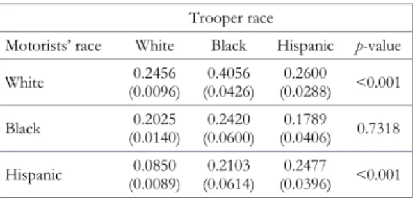
Finally, Table 2 reproduces Panel B in AF’s Table 1 using 1,000 instead of 30 iterations. Like the rates in AF, the rates in Table 2 stem from one particular pass and are therefore random. However, because the possible ranges into which these estimates can fall are now considerably narrower, the results are more robust.
Figure 5. Relationship between precision of estimated average search-success rate and number of iterations used
TABLE 2. Estimated average search-success rates with 1,000 iterations
Trooper race
Motorists’ race White Black Hispanic p-value White (0.0096)0.2456 (0.0426)0.4056 (0.0288)0.2600 <0.001
Black (0.0140)0.2025 (0.0600)0.2420 (0.0406)0.1789 0.7318
Hispanic (0.0089)0.0850 (0.0614)0.2103 (0.0396)0.2477 <0.001
Note: Standard errors of the means are shown in parentheses.
Appendix 2: An alternative randomization test
To test the estimated rates, AF employ conventional χ2 and difference of means tests. But although increasing the number of iterations allows for more conclusive inferences based on the estimates, it is not clear if these tests are applicable here in the first place as they assume the baseline values to be non-stochastic. Statistically speaking, there exists no formal basis for concatenating the random outcomes with the employed empirical tests. In this section, I propose an alternative rank order test for use in determining how likely it is that the observed differences in the rank orders are purely by chance.
The very nature of the resampling procedure lends itself to a preceding randomization construction.29In devising a null distribution from the data them-selves, we can obtain an exact answer to the question of how likely the observed values would be if the null hypothesis were true. The null distribution is con-structed by randomly rearranging the labels of the observations. If under the null hypothesis these labels do not matter, their permutation should not change the distribution of the original data. Such nonparametric randomization tests date back to Fisher (1935).30With the recent rise in computational power, they have become increasingly popular in applied statistics. The method has the advantage that it does not require specific assumptions about the underlying distributions. Moreover, it can be applied to make inferences about arbitrarily complicated test statistics, such as our resampled, aggregated, and finally averaged search-success rates.
The null hypothesis in AF’s rank order test states that the search-success rates against a given race of motorists do not depend on the race of the troopers (AF 2006, 146). To implement this null hypothesis in the randomization test, I
reshuffle the trooper identifier labels in the raw search data prior to the merger with the trooper subsamples.31Confining the reshufflings separately within troop and motorist race blocks picks up any potentially specific effects. This preceding randomization mirrors the idea that if the search-success rates do not depend on the race of the troopers searching them, reassigning the searches to troopers of different races should have no effect on the distribution of the search-success rates.32
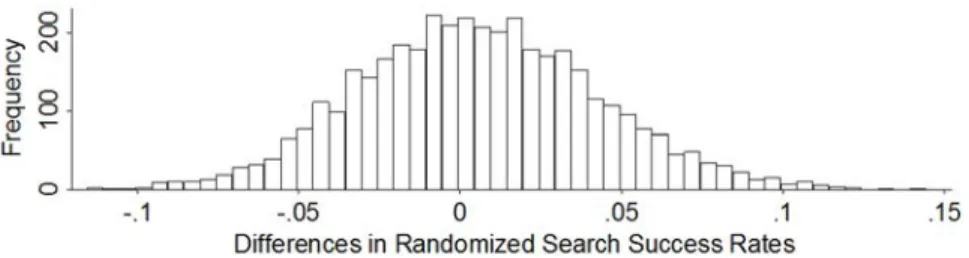
Our observed values of the test statistic are the pairwise differences in search-success rates for a given race of motorists from Table 2. Under the null, these differences are zero. The corresponding null distributions are constructed by running a large number of independent passes, each of which is preceded by the randomization. After each pass, the differences in the search-success rates for a given race of motorists are recorded, providing the null distributions in which trooper race is exchangeable. In each null distribution, I calculate the exactp-value as the proportion of random values that are at least as extreme as the observed value. If trooper race does not matter, one should rarely find differences as large as the observed one. As an example, Figure 6 shows the frequency distribution in randomly obtained differences of the rates of Hispanic and white troopers against black motorists. It is easy to see that the observed value in Table 2, 0.1789 − 0.2025 = −0.0236, is not unusual when compared to this null distribution.
Figure 6. Null distribution of differences in search-success rates of Hispanic and white troopers against black motorists
31. In contrast to my replication of AF’s resampling procedure, the implementation of the randomization test required truly random seeds, which were obtained via the Stata packagesetrngseed.
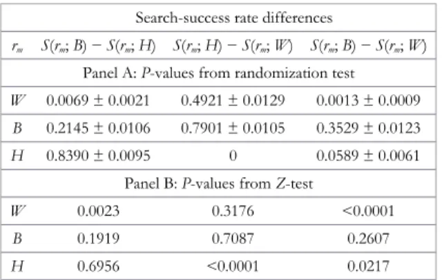
Panel A in Table 3 contains the estimated p-values for all differences in average search-success rates from the randomization test using 10,000 passes (with 1,000 iterations each). Thep-values include their 99-CI.33For ease of comparison with AF’s parametric test, thep-values from the replicatedZ-tests based on Table 2 are shown in Panel B of Table 3. I follow AF’s notation of search-success ratesS(rm;
rp, wherermandrp∈{W,B,H} denote the motorist and trooper races, respectively.
For a given race of motorists, the first column in Table 3 tests whether we can reject the null hypothesis of equal search-success rates for black and Hispanic troopers in favor of the one-sided alternative that black troopers exhibit a higher rate. The second column tests for inequality between Hispanic and white troopers. In addition, the third column tests for inequality between black and white troopers—the first and third rank.
TABLE 3.PP-values of differences in search-success rates
Search-success rate differences
rm S(rm;B) −S(rm;H) S(rm;H) −S(rm;W) S(rm;B) −S(rm;W)
Panel A:P-values from randomization test
W 0.0069 ± 0.0021 0.4921 ± 0.0129 0.0013 ± 0.0009
B 0.2145 ± 0.0106 0.7901 ± 0.0105 0.3529 ± 0.0123
H 0.8390 ± 0.0095 0 0.0589 ± 0.0061
Panel B:P-values fromZ-test
W 0.0023 0.3176 <0.0001
B 0.1919 0.7087 0.2607
H 0.6956 <0.0001 0.0217
By and large, the statistical inferences from the randomization tests are consistent with the ones from AF’s empirical tests based on AF’s generalized resampling procedure in Appendix 1. The p-values retain their levels of significance, with the exception of one rank. Using the randomization test, we cannot formally reject equality between the average search-success rates of black and white troopers against Hispanic motorists at a five percent level of significance: Thep-value from theZ-test, 0.022, rises to 0.056. But for all intents and purposes, it still remains unlikely that this difference has been brought about purely by chance.
33. Calculating all possible permutations would yield exactp-values but is computationally not feasible. Even so, a randomization test is asymptotically equivalent to such an exact test when the number of randomized passes is large enough. The precision of the estimated p-value,p̂, increases with the number of passes. From the binomial distribution, the standard error ofp̂is given bySEp̂= [p̂(1 −p̂)(1/n)]½wheren
Appendix 3: Data and code files
On theEcon Journal Watchwebsite isa guide to all the data and code files used in this research.
References
Anwar, Shamena, and Hanming Fang. 2006. An Alternative Test of Racial Prejudice in Motor Vehicle Searches: Theory and Evidence. American Economic Review96(1): 127-151.Link
Arrow, Kenneth J. 1973. The Theory of Discrimination. InDiscrimination in Labor Markets, eds. Orley Ashenfelter and Albert Rees, 3-33. Princeton, N.J.: Princeton University Press.
Becker, Gary R. 1957. The Economics of Discrimination. Chicago: University of Chicago Press.
Close, Billy R., and Patrick L. Mason. 2007. Searching for Efficient Enforcement: Officer Characteristics and Racially Biased Policing.Review of Law and Economics3(2): 263-321.
Fisher, Ronald A. 1935.The Design of Experiments. London: Oliver & Boyd. Ilić, Dragan. 2013. Spatial and Temporal Aggregation in Racial Profiling.Swiss
Journal of Economics and Statistics149(1): 27-56.
Knowles, John, Nicola Persico, and Petra Todd. 2001. Racial Bias in Motor Vehicle Searches: Theory and Evidence.Journal of Political Economy 109(1): 203-229.
Persico, Nicola, and Petra Todd. 2006. Generalising the Hit Rates Tests to Test for Racial Bias in Law Enforcement, with an Application to Vehicle Searches in Wichita.Economic Journal116: F351-F367.
Phelps, Edmund S. 1972. The Statistical Theory of Racism and Sexism.American Economic Review62: 659-661.
Romano, Joseph P. 1990. On the Behavior of Randomization Tests Without a Group Invariance Assumption.Journal of the American Statistical Association
85(411): 686-692.
Wu, Chien F. J. 1990. On the Asymptotic Properties of the Jackknife Histogram.
Dragan Ilićis lecturer and senior researcher in the Economic Theory Group of the Faculty of Business and Economics at the University of Basel. His research interests are applied microeconomics and social economics. His email address is [email protected].
About the Author
Go to archive of Comments section Go to September 2014 issue
Discuss this article at Journaltalk:
Saying Too Little, Too Late:
Public Finance Textbooks and
the Excess Burdens of Taxation
Cecil E. Bohanon
1, John B. Horowitz
2, and James E. McClure
3LINKTO ABSTRACT
Taxation imposes manifold costs beyond the amount of revenue raised. During recent decades economists have investigated the excess burdens of taxation including the costs of ‘deadweight’ distortions, enforcement, and compliance.4Our synthesis of the estimates provided by these investigations indicate that it typically costs much more than a dollar to finance a dollar of government spending. We examine whether leading public finance textbooks discuss the various excess bur-dens or incorporate excess burbur-dens when calculating the optimal level of public goods. We find that most do neither.
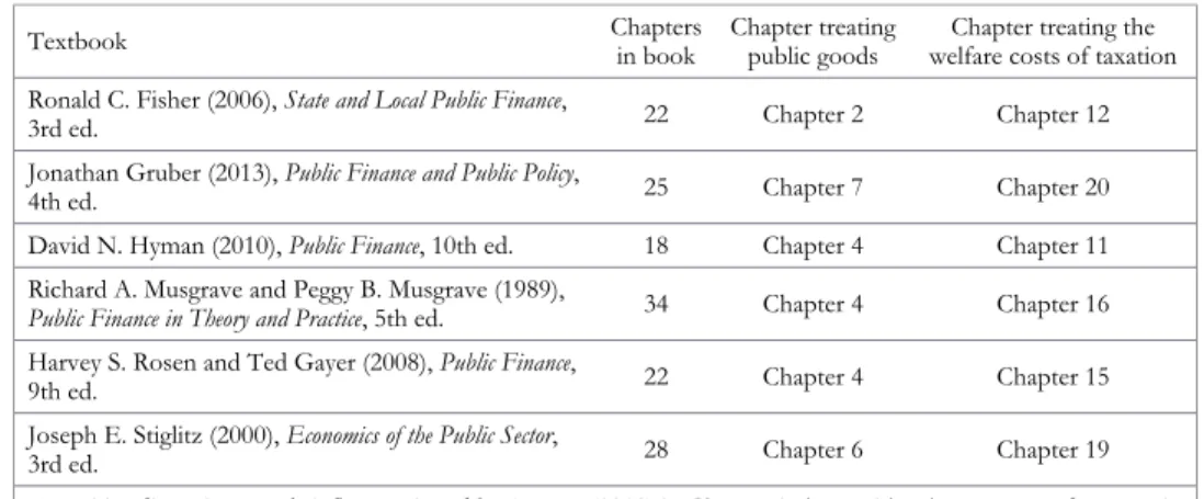
Table 1 gives the locations of the treatments of (1) public goods and (2) the welfare costs of taxation found in six public finance textbooks used in top economics programs in the United States.5In each of the six books, the treatment of public goods precedes the treatment of the welfare costs of taxation (tax efficiency). In fact, after treating public goods, the treatment of tax efficiency comes, on average, 11 chapters later. By the time the author(s) gets to tax efficiency, the focus has long since shifted away from the optimal provision of public goods.
ECON JOURNAL WATCH 11(3)
September 2014: 277-296
1. Ball State University, Muncie, IN 47306. 2. Ball State University, Muncie, IN 47306. 3. Ball State University, Muncie, IN 47306.
4.SeeSlemrod and Gillitzer (2014) for an in-depth discussion of administrative, compliance, and welfare costs of taxation.
TABLE 1. Topic separation: Public goods vs. the welfare costs of taxation
Textbook Chaptersin book Chapter treatingpublic goods welfare costs of taxationChapter treating the
Ronald C. Fisher (2006),State and Local Public Finance,
3rd ed. 22 Chapter 2 Chapter 12
Jonathan Gruber (2013),Public Finance and Public Policy,
4th ed. 25 Chapter 7 Chapter 20
David N. Hyman (2010),Public Finance, 10th ed. 18 Chapter 4 Chapter 11 Richard A. Musgrave and Peggy B. Musgrave (1989),
Public Finance in Theory and Practice, 5th ed. 34 Chapter 4 Chapter 16 Harvey S. Rosen and Ted Gayer (2008),Public Finance,
9th ed. 22 Chapter 4 Chapter 15
Joseph E. Stiglitz (2000),Economics of the Public Sector,
3rd ed. 28 Chapter 6 Chapter 19
Note: Tax distortions are briefly mentioned by Hyman (2010) in Chapter 2 along with other sources of economic distortions.
The sequencing and wide separation of these discussions is a manifestation of the broader problem we focus upon: Textbooks say too little, too late, about the excess burdens of taxation. Even when the textbooks do get around to treating tax efficiency, the coverage of the costs of taxation is often inadequate. Such practice is likely to lead students to underestimate the costs of government programs, predisposing them toward increased government spending.6 If instead students were instructed on the manifold costs of taxation and these costs were integrated into discussions of public goods, students would probably be less predisposed toward government spending.
Naive public goods theory misleads on costs
Just like the modern textbooks, Adam Smith’s Wealth of Nationsdiscusses government expenses first and then turns to revenue (Smith 1976/1776, V.1, V.2). However, unlike the modern textbook writers, when Smith discussed expenses he consistently integrated some discussion of their financing. Smith quite consistently preferred such financing to come principally from user fees, though Smith did consider national defense to be a pure public good that should be financed by
general taxation. Thus for Smith the relevance of tax efficiency to public goods should perhaps be limited, while its relevance should be high to modern textbook writers, who more often tend to favor general taxation as the financing mechanism when public goods are demanded.
In their analysis of public goods, textbooks normally depict supply as a marginal cost curve that does not include excess burdens. They normally assume lump-sum taxation with full information, though typically they do not make this explicit. This depiction may be reasonable when politicians are hammering out this year’s budget and deciding how to allocate money between programs. However, the depiction is not suitable in discussions of the optimal provision of a public good. Government must raise revenue to provide public goods, and so to assume a nondistortionary lump-sum tax will lead students to overestimate optimal provision.
When textbooks leave excess burdens unmentioned, they are de facto teach-ing the lump-sum tax perspective. The author of a textbook might deny assumteach-ing nondistortionary taxes, declaring ‘Just because I didn’t elaborate the manifold costs doesn’t mean I have denied such costs; rather, they are implicitly represented in the marginal-cost curve.’ We think that such a defense is inadequate. Normally governments must raise the revenue to provide the public good. Raising revenue generates enforcement costs, compliance costs, and deadweight distortions. When textbook authors don’t explicitly discuss these costs when discussing the optimal provision of a public good, it leads students to forget that taxes are distortionary and ignore these welfare costs when doing their analyses.
Adam Smith on the excess burdens of taxation
Smith’s four maxims of taxation underscore the excess burdens of taxation. Smith’s brief presentation of these maxims comes at the very beginning of his lengthy treatment of taxation: “Before I enter upon the examination of particular taxes, it is necessary to premise the four following maxims with regard to taxes in general” (1976/1776, 825).
The second maxim is that tax obligations “ought to be certain, and not arbitrary. The time of payment, the manner of payment, the quantity to be paid, ought all to be clear and plain to the contributor, and to every other person” (ibid.). Without certainty, Smith says, the tax-gatherer “can either aggravate the tax upon any obnoxious contributor, or extort, by the terror of such aggravation, some present or perquisite to himself. The uncertainty of taxation encourages the insolence and favours the corruption of an order of men who are naturally unpopular” (ibid., 825-826). Smith argues that certain and non-arbitrary tax payments reduce the excess burdens of taxation.
The third maxim is that “Every tax ought to be levied at the time, or in the manner, in which it is most likely to be convenient for the contributor to pay it” (ibid., 826). Here Smith clearly highlights excess burden. He says that taxes “upon the rent of land or of houses” or “upon such consumable goods as are articles of luxuries” are conveniently paid.
The fourth maxim is more elaborate and broken down into four sub-points. It is entirely and explicitly about excess burden, including the psychic costs arising from “trouble, vexation, and oppression.” We quote the paragraph in full:
which ought certainly to alleviate it, the temptation to commit the crime. Fourthly, by subjecting the people to the frequent visits and the odious examination of the tax-gatherers, it may expose them to much unnecessary trouble, vexation, and oppression; and though vexation is not, strictly speaking, expence, it is certainly equivalent to the expence at which every man would be willing to redeem himself from it. It is in some one or other of these four different ways that taxes are frequently so much more burdensome to the people than they are beneficial to the sovereign. (Smith 1976/1776, 826-827)
No contemporary public finance textbook that we are aware of even comes close to discussing excess burdens as comprehensively as Smith did in 1776.
Some analysis and estimates
of the excess burden
One would like to think that economists can neatly distinguish the com-ponents of the excess burden of taxation, provide a precise estimate of the magnitude of each component, and then add up the component estimates to arrive at an estimate of the total excess burden.7Unfortunately, for a number of reasons it is not that simple. Consider some of the complicating factors. First, cost depends on how the relevant choice is contextualized.8Second, taxation takes many forms. Third, it is very difficult to arrive at monetary values for the subjective costs from fear, anxiety, anger, and frustration from what Smith called “unnecessary trouble, vexation, and oppression.” Fourth, there is no definitive way to divide the components; for example, should enforcement be separated from compliance? Fifth, some potential components, such as ones having to do with tax evasion, tax avoidance, or black markets, might mitigate other components, such as suppressed work or opportunity. Sixth, empirical estimation is necessarily very crude and inexact. Seventh, the costs vary over time; for example, perhaps technology is making it easier for people to comply with tax law.
One component of excess burden is compliance cost, the costs of con-forming to often complex and changing tax laws. Joel Slemrod and Jon Bakija estimate that “individual taxpayers spend as much as 3billionhours of their own
7. For a breakdown of components and estimates, see James Payne (1993, 150, 247-248). Incidentally, Payne insists that all of his estimates are conservative, lower-bound estimates (ibid., 9).
time on tax matters, or about 27 hours per taxpayer on average. That is the equivalent of over 1.5 million full-time (but hidden and unpaid) IRS employees!” (2008, 3-4, emphasis in original). The IRS (2012, Table 2.1) reports that tax preparation fees reported as itemized deductions were about $6.9 billion. Slemrod and Bakija (2008, 162) report that their “best estimate of the total annual cost of enforcing and complying with the federal corporate and personal income taxes in tax year 2004 is $135 billion. This amounts to slightly more than 10 cents per dollar raised.” In other words, for each dollar collected via income taxes, the inclusion of compliance costs alone would bring the total burden to $1.10.9
Tax wedges are another important cost of taxation. In labor markets, the average taxpayer works less when she faces higher marginal tax rates. Although average tax rates are easily used to calculate one’s tax bill from gross income, the effects of taxes on one’s decisions to work and save are determined by the overall
marginal tax rate (MTR) from federal, state, and local taxes.10 Edward Prescott (2004) reported that in 1970 labor supplies were nearly equal in the United States and Europe. Also in 1970, MTRs were similar in the United States and Europe. By the mid-1990s, MTRs in Europe increased to about 60 percent, compared to 40 percent in the United States—and Europeans were working about a third less than Americans. Prescott (2004, 8) finds that much of the difference in labor supply is explained by the differing MTRs.
Some analysts discuss disincentives to save as another cost of taxation; higher MTRs reduce the incentive to save. Taxes on dividends, capital gains, interest income, and corporate and business profits reduce savers’ rates of return. Although there is little agreement on how much these taxes affect savings, Jonathan Gruber (2013) notes that more recent studies suggest that consumption decisions are strongly affected by after-tax interest rates. Edgar Browning (2008) argues that one reason Americans save less than many other countries is the relatively high American MTRs on capital income. Progressive taxes also place the largest tax burden on higher income people who tend to save the most. Browning (2008) says that total savings is especially reduced by progressive taxes that reduce the return to savings for high-income individuals, who tend to save the most.
9. Payne (1993) made a much higher estimate of compliance costs borne by households and businesses, about 24 cents per tax-revenue dollar. Payne separately estimated enforcement costs, meaning the “governmental cost of tax collection,” but he found they “prove to be relatively small.” He added: “Virtually all of the costs of operating the U.S. tax system are shifted onto the private sector” (Payne 1993, 9, 29, see also 119-126).
Distortions arising from reductions in the tax base via exemptions and deductions are another matter sometimes treated as a cost of taxation. According to the Internal Revenue Service (2013, Table 5), adjusted gross income since 1970 is 15% to 25% less than personal income. Taxpayers have the incentive to move their income into areas that are not taxed. This distorts taxpayers’ choices.
The welfare costs of taxation cannot be measured with great precision. Bev Dahlby (2008) presents various estimates of the marginal costs of public funds (MCF) for various taxes. But MCF is only one of several frameworks that have been used in measuring the welfare costs of taxation; others include marginal excess burden (MEB), marginal efficiency costs (MEC), and marginal welfare costs (MWC). This makes it difficult to summarize and compare the results from the various studies.
Table 2 lists the results from nine publications that assess the costs of raising tax revenue from labor income in the United States. Over the last thirty years, individual income and payroll taxes have been the source of at least eighty percent of all federal tax revenue (OMB 2014, 34-35). Column 2 shows estimates of the cost of raising a dollar in income tax revenue when compliance costs are excluded; estimates range from $1.07 to $1.52, with one outlying high estimate of $3.00. As discussed, Slemrod and Bakija (2008) estimate that there is a $0.10 compliance cost when raising a dollar in tax revenue; column 3 thus includes compliance costs by adding ten cents to the estimates in column 2.
TABLE 2. Estimates of the cost of raising a dollar in tax revenue from a labor income tax
Source for estimate (1)
Estimate (excludes compliance costs)
(2)
Estimate plus compliance costs of $0.10
(3) Ahmed and Croushore (1996) $1.12 to $1.17 $1.22 to $1.27 Ballard, Shoven, and Whalley (1985) $1.16 to $1.31 $1.26 to $1.41 Browning (1987) $1.32 to $1.47 $1.42 to $1.57
Feldstein (1999) $3.00 $3.10
Fullerton and Henderson (1989) $1.17 to $1.25 $1.27 to $1.35
Gruber and Saez (2002) $1.29 $1.39
Jorgenson and Yun (1991) $1.38 to $1.52 $1.48 to $1.62 Jorgenson and Yun (2001) $1.35 to $1.40 $1.45 to $1.50
Stuart (1984) $1.07 $1.17
Median $1.29 to $1.31 $1.39 to $1.41
Average $1.43 to $1.50 $1.53 to $1.60
Considering all nine publications, the median estimate of the cost to raise a dollar in revenue through a tax on labor income (column 2) is about $1.30; including ten cents of compliance costs, the figure is about $1.40 (column 3). A $1.40 cost to raise a dollar in income tax revenue implies that textbook writers who assume that it costs a dollar to raise a dollar are ignoring about 30 percent of the costs.
These estimates do not seem to be controversial. In 2005, the President’s Council of Economic Advisers reported: “A recent study estimated that the excess burden associated with increasing the individual income tax by one dollar is 30 to 50 cents. In other words, the total burden of collecting $1.00 in additional income taxes is between $1.30 and $1.50, not counting compliance costs” (Bush CEA 2005, 77). In aJournal of Economic Literaturereview, Slemrod (2005, 817) said this estimate cited by the CEA “is a reasonable characterization of where the literature stands.”
The costs of raising funds through a general sales tax are similar. Charles Ballard, John Shoven, and John Whalley’s (1985) estimate of the MEB for consumer sales taxes puts the cost of raising a dollar of public funds between $1.25 and $1.39. Dale Jorgenson and Kun-Young Yun (1991) estimate the MEC of a sales tax on consumer and investment goods to be about $1.26; in later work, Jorgenson and Yun (2001) estimated the MEC to be about $1.18. All of these estimates omit compliance and enforcement costs, so the full cost of raising a dollar of public funds would be even higher.