ISSN 2319-7617 (Online)
(An International Research Journal), www.physics-journal.org
Study of Abrikosor Vortex lattice and evaluation of
and
as a function of reduced temperature
cfor
two N
b-T
1superconductor
Shambhoo Nath Prabhakar
Department of Physics,
Mahila College, Tekari (Gaya), Vill : Andhar : P.O- Makhdumpur- 824232, INDIA. email: [email protected].
(Received on: November 27, 2018)
ABSTRACT
Type- I Superconductor are superconductors that exhibit zero resistance and perfect diamagnetism. They are perfect diamegnets for applied magnetic fields below the critical field Bc and becomes normal for higher applied fields. Their coherence
length exceeds their penetration depth ( > ) so it is not energically favourable for boundaries to form between their normal and superconducting phase. The superconducting element with the exception of Niobium, are all type I.
When the penetration depth is larger than the coherence length , it becomes energetically favorable for domain walls to form between the superconducting and normal regions. When such a superconductor, called type II, is in a magnetic field, the free energy can be lowered by causing domains of normal material containing trapped flux to form with low energy boundaries created between the normal core and the surrounding superconducting material. When the applied magnetic field exceeds a value referred to as the lower critical field, BC1, magnetic
field is able to penetrate in quantized units by forming cylindrically symmetrical domains called vortices. For applied fields slightly above BC1 the magnetic field inside a type II superconductor is strong in the normal cores of the vortices, decreases with distance from the cores, and becomes very small far away for much higher applied field the vortices overlap and the field inside the superconductor become strong everywhere. Eventually, when the applied field reaches a value called the upper critical field BC2, the materials becomes normal. Alloys and compounds exhibit type
above BC1. Type II superconductors also have zero resistance, but their perfect
diamagnetism occurs only below the lower critical field BC1. Then one defines the
ratio of and as a Ginzburg-Landau parameter K. K plays a very important role in
type II superconductors. The density of super electron ns which characterizes the
superconducting state, increase from zero at the interface with a normal material to a constant value for inside, and the length scale for this to occur is the coherence length . As external magnetic field B decays exponential to zero inside a superconductor. For type I superconductor for coherence length is the larger of the two length scales, so superconducting coherence is maintained over relatively large distance within the sample. The overall coherence of the superconducting electrons is not disturbed by the presence of external magnetic fields.
Keywords: Superconductivity, super current, vortex lattice, Gibbs energy.
INTRODUCTION
We have discussed in great detail about GL equation in chapter II. In fact one has given an account of calculation of second order critical fields with the use of limearized GL equations. We have HC2= K√2 Hcb. Within the framework of GL theory1, k is independence.
There is another field HC3 where superconductivity appears in the form surface sheath with a
with a thickness above coherence length ( ) on surface parallel to the applied field. Our has Hc3 = 1.69 k√2 Hcb = 1.69Hc2. Between Hc2 and HC3 a super current can flow in the surface
sheath, so that the resistance transition for a small measuring current occurs at HC3. The
magnetization on the other hand is governed by the behavior of the bulk of the specimen2. So
that the magnetic transition occurs at HC2. In type I superconductor which has HC2<Hcb<Hc3
may be expected to appear as the critical supercooling field. It is also possible to have intermediate type superconductor with Hc2<Hcb<Hc3 in which the surface sheath appears in
some field interval above Hcb.
Now at HC2 and HC3. The order parameter varies spatially, over the characteristics
distance ( ) whereas in calculating the critical field of a film of thickness d< ( ),one is able to take Ψ as a constant. Now one goes to look at some consequences of the nonlinear term
β|Ψ|2 Ψ in the GL equation. In particular, one discusses the structure of the mixed state. Ψ
various spatially and it is not possible to deal analytically with the nonlinear terms for all values of Ho. However, one is dealing with the second order phase transition, and just however, Hc2. Ψ is small so that one can handle the nonlinear terms by a perturbation method. The solution of the problems is due to Abrilcosov3. In this chapter, we have discussed the Abrikosov vortex
lattice and evaluated the ratio of and as a function of reduced temperature (T/Tc) for two Nb-Ti alloys. Our evaluated values of these two ratio decreases of (T/Tc). The
MATHEMATICAL FORMALUE USED IN THE EVALUATION
Now one uses first- Ginzburg-Landau equation which is given by
(- it ∇ - 2eA)2ψ + αψ|β|2ψ =0 (1)
With the use of garge div A= 0. A is the vector potential. The expression for current density is given by
Jc = ћ
(ψ*∇ψ - ψ∇ψX) - ψxψA (2)
This is the standard expression for a quantum mechanical current Here A enters only
in the gradient terms and in the field energy terms 2 . Here one uses the mass m rather
than 2m which means only a change in the normalization of ψ. Equation (2) indicates that a superconductor is characterized by a macroscopic wave function. Equation (3) is a type of local expression.
We have to solve the two GL equation (3) for ψ and (2) for the current Je. We take the
applied field Ho to be just less than Hc2. So that the vector potential A satisfies.
Curl A = B = 0 Ho + Bloc (3)
Where Bloc is the field generated by the super currents.
Curl Bloc = 0 Je (4)
It is convenient to write
A = Ac2+A1 (5)
Where Ac2 is the vector potential of the field Hc2. Given by
Ac2 = (0, = 0 Hc2X,0) (6)
We take all magnetic fields to be directed along the z axis.
Just below Hc2. We can expect ψ to be close to a solution of the linear equation (6), with Hc2,
in place of H0. We therefore put
ψ = ψL + ψ1 (7)
Where ψL is solution of the linear equation. However, equation (7) begs tow questions about
ψL is important because we have a nonlinear system, the normalization of ψL is important eventually the normalization determines the strength of the super current Je and therefore the
induction B. To make sure that we have the correct normalization, we shall require ψL and ψ1
are orthogonal ∫ Lψ1 d3 r= 0 (8)
We can expand ψ1 as a series in terms of the eigenfunctions for the oscillator Hamiltonian, and equation (8) is the condition that the lowest eigenfunction ψL does not occur in ψ1. The second equation about ψL arises because the lowest eigenstate is highly degenerate the solution can have any values of ky and xo. Again the nonlinearity of the system lifts the degeneracy, and
singles out one particular solution. At the outset, however, we simply choose a general linear combination of solutions with various xo values.
ψL (x,y) = ∑ n exp (inky) exp [ -(x-xn)2 / 2 2(T)] (9)
with
It will be seen that equation (9) is periodic in y with wavelength 2 /k. Following the original calculation of Abrikosov, we shall consider only combination such that |ψL|2 is periodic in x as well as in y. We can ensure this with the periodicity condition.
Cn+N = Cn (11)
In fact the only value of N that have been considered are N=1 (Abrikosv 1957)3 and N= 2 (Kleiner et al 1964)4 the latter given the triangular lattice which is observed in practice. The choice of a periodic solution in (11) is nowadays rather obvious that the mixed state consists of a periodic array of vortices.
Most of the analysis is independent of the details structure of ψL that is the particular choice of Cn and k in equation (8). The first important result concerns the current JL associated
with ψL. If equation (9) is substituted into equation (2) for the current, it can be shown that
JLx = - |ψL|2 (12)
JLy = - |ψL|2 (13)
This means, by comparison with equation (4), that the field generated by JL, which is the z
direction of course is
Bloc = - 0 eћ|ψL|2 / m (14)
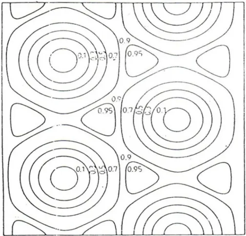
This gives us the important result that the lines of constant B coincide with the lines of constant |ψL|2, and that these lines are also the lines of current flow, J
L. Thus the contours in diagrams
like figure (A) and (B) represent at the same time level surface |ψL|2 and of B and streamlines of the current JL.
We can now look at the normalization of ψL. We slipt us A and ψ as in equations (5) and (7), and rewrite the GL equation for ψ as an equation for the small correction ψ1 :
(- iћ∇-2eAc2)2ψ1 + αψ1 + (- iћ∇ - 2eAc2 - 2eA1-)2 ψL
+αψL+β|ψL|2ψL = 0 (15)
We treat, A1, ψL and β|ψL|2. As small quantities, and retain only first-order terms. For
convenience, we have kept in the zeroth-order term HoψL, where
Ho= (- iћ∇ - 2eAc2 )2 +α (16)
We have
Hoψ L = 0 (17)
Since this is the defining equation for ψL. The term involving ψ1 in equation (15) is Hoψ1. It
we think again of ψ1 as a sum of eigenfunctions of Ho, not including ψL. Hence our normalization condition, equation (8) is equivalent to
∫ *
L Hoψ1d3r = 0 (18)
We can substitute for Hoψ1 from equation (15), to get the explicit form
∫ ∗(− ћ∇ −2 −2 ) + | | + | | d3r = 0 (19)
In order to make the solution explicit, we have to reorganize equation (19) somewhat. First, we integrate the first term by parts, to introduce ∇ ∗ . The zeroth-order part of the first term cancels the integral of α| | , and the rest, ignoring the term in , gives
∫(− . + | | ) d3 r = 0
Where JL as before, is the current associated with ψL . With the use of equation (7) the first term here is
∫ = − ∫ (20)
= 1 ∫ . Curl A1 d3 r (21)
Where again we have integrated by parts, using the vector identity div (AxB) = B. Curl A-A. curl B. Form equation (3) and (5) we have.
CurlA1 = (Ho – Hc2) + Bloc (22)
Putting equation (22) and (21) into equation (20) and using equation (14) for Bloc, we find
(2 −1) <| | >= ( − ) < | | > (23) Where we have introduced the notation
∫| | = 〈 〉2
etc. (24)
and replaced β by K2
Equation (23) essentially as far as we can go without investigating the detailed form of the flux lattice described by ψL. It is convenient to summaries the properties of the lattice, following Abrikosov, in the parameter βA :
βA = 〈| | 〉/ (〈| | 〉 ) (25) Clearly we have β≥1 for any form of ψL. Equation (23) then yield
〈| | 〉 = ( ) (26)
The average induction, from equation (3) and (14) is
〈 〉 = −
( ) (27)
and equivalently the magnetization is
M = ( ) (28)
It is easy to see from equation (28) that the Gibbs energy G decreases as βA decreases. The choice of the parameters Cn and k in equation (9) must therefore be made in such a way
as to minimize βA. Abrikosvo originally chose all Cn equal and k = (2 )1/2 / (t), which gives
a square lattice, illustrated in figure 3A with βA = 1.18. Later, Klenier et al (1964)1 showed that the choice N=2 in the periodicity equation (11) together with
C1 = ± iCo (29)
Which corresponds to a triangular lattices give BA = 1.16. Furthermore, the square lattice can
be sheared continuously into the triangular lattice with BA decreasing all the time, so that there
Perhaps the most important features of the results we have just derived is that the magnetization, equation (28) depends upon the same parameters K as gives the critical field Hc2. The GL equation, in the form in which we have stated them, are obviously valid only in
some temperature interval near Tc. Since we started with Landau’s assumption that the free
energy can be expanded as a power series in the order parameter. In fact, for alloys, in which the electrodynamics are local, the microscopic theory can be solved at all temperatures of H ~ Hc2, using a method based on the Abrikosov calculation. The result is that the equation for Hc2.
And the magnetization M continue to hold, except that the K parameter involved are different function of temperature.
Hc2 = K1 (T) √2 Hcb (30)
M = - ( )
( ) (31)
From this more recent point of view, one can say that the result of the GL calculation is that the K parameters coincide at T = Tc.
DISCUSSION OF RESULTS
In this paper, we have studied the Abrikosov vortex lattice and evaluated the ratio of
and for two Nb-Ti alloys smaple superconductor. We have taken the value of
k from Gizburg. Landau values. The evaluation has been performed as a function of reduced temperature . The results are shown in table 3T1 and 3T2 respectively for the given two
samples. Our theoretical results indicated the ratio and both reduces as a
function of . Coincides at T= Tc. The limiting values of Tc is the same for both. These
results are consistent with the theoretical results of other workers 6-15
Table: 1
Evaluation of and as function of reduced temperature for Nb-Ti alloy 37% (sample I) superconductor k = 0.84 is the GL Value
0 1.55 2.50
0.1 1.50 2.40
0.2 1.46 2.10
0.3 1.42 2.00
0.4 1.40 1.89
0.5 1.38 1.80
0.6 1.36 1.70
0.7 1.36 1.70
0.8 1.32 1.50
0.9 1.30 1.40
Table: 2
Evaluation of and as function of reduced temperature for Nb-Ti alloy 43% (sample II) superconductor k = 0.84 is the GL Value
0 1.40 2.55
0.1 1.32 2.50
0.2 1.28 2.45
0.3 1.26 2.37
0.4 1.22 2.33
0.5 1.20 2.30
0.6 1.18 2.27
0.7 1.16 2.23
0.8 1.14 2.20
0.9 1.13 2.18
1.0 1.12 2.16
Figure: 1 Level surfaces of |ψL|2 for the Abrikosov square lattice. The axes are marked in units of (2 )1/2
Figure 2 : Level surfaces of |ψL|2 for the triangular lattice. The vertical distance between vortex cores is
2 1/2 (T)/31/4 and the horizontal distance between the rows of vortices is 31/4 1/2 (T). (From Kleiner et al
1964).
CONCLUSION
As a from problem we have studied the Abrikosov we have studied the Abrikosov
vortex lattice and evaluated the ratio of and for two Nb-Ti alloys sample
superconductor. We have taken the value of k from Gizburg. Landau values. The evaluation
has been performed as a function of reduced temperature . The results are shown in
table 1 and 2 respectively for the given samples. Our theoretical results indicates that the ratio
and both reduces as a function of , The decrease is more pronounced
for higher value of , Coincides at T=Tc. The limiting values of Tc is the same for both.
REFERENCES
1. V.L. Ginzburg and L.D. Landau, Zh. Eksp. Teor. Fiz 20, 1064 (1980).
2. I.I. Geguizin, I. Ya Nikitoror and G.I. Alperoviteh, Fiz. Tvend Tela 15, 931 (1973). 3. A. A. Abrikosov, Sov. Phys. JETP 5 1174 (1957).
4. W.H. Kleiner, L.M. Rott and S. H. Autler, Phys. Rev. 133A 1226 (1964). 5. U. Essmann and H. Trauble, Phys. Lett. 24A, 526 (1967).
6. D. Goldschmidh Phys Rev B39. 2372 (1989).
7. A. Gold and A. Ghazali, Phys Rev. B43m 12952 (1991).
8. J.B. Goodenough, HJ.S. Zhou and J. Chan, Phys. Rev B 47. 5275 (1993).
9. N. H. Huer, N.H. Kim, S.H. Kim, Y.K. Park and J.C. Park, Physica C 231 227 (1994). 10. B.I. Ivlev and R.S. Thompson, Phys. Rev. B 57, 875 (1995).
11. Z. Iqbal, Supercond. Rev. 5, 49, (1996).
12. F. Irie and K. Yamtuji, J. Phys. Soc. Jpn. 63, 255 (1996). 13. K.P. Jain and D.K. Ray, Phys. Rev. 55, 12322 (1996). 14. S. Kivebon. Physica C 234, 567 (1996).