General Rights
Copyright and moral rights for the publications made accessible in the public portal are retained by the authors and/or other copyright owners and it is a condition of accessing publications that users recognize and abide by the legal requirements associated with these rights.
• Users may download and print one copy of any publication from the public portal for the purpose of private study or research. • You may not further distribute the material or use it for any profit-making activity or commercial gain
• You may freely distribute the URL identifying the publication in the public portal
If you believe that this document breaches copyright please contact us providing details, and we will remove access to the work immediately and investigate your claim.
If the document is published under a Creative Commons license, this applies instead of the general rights.
Coversheet
This is the accepted manuscript (post-print version) of the article.
Contentwise, the accepted manuscript version is identical to the final published version, but there may be differences in typography and layout.
How to cite this publication
Please cite the final published version:
Soroush Alamdari, Patrizio Angelini, Fidel Barrera-Cruz, Timothy M. Chan, Giordano Da Lozzo, Giuseppe Di Battista, Fabrizio Frati, Penny Haxell, Anna Lubiw, Maurizio Patrignani, Vincenzo Roselli, Sahil Singla, and Bryan T. Wilkinson (2017). How to Morph Planar Graph Drawings. In SIAM Journal on
Computing 46(2), 824-852.
DOI: https://doi.org/10.1137/16M1069171
Publication metadata
Title: How to Morph Planar Graph Drawings
Author(s): Soroush Alamdari, Patrizio Angelini, Fidel Barrera-Cruz, Timothy M. Chan, Giordano Da Lozzo, Giuseppe Di Battista, Fabrizio Frati, Penny Haxell, Anna Lubiw, Maurizio Patrignani, Vincenzo Roselli, Sahil Singla, and Bryan T. Wilkinson
Journal: SIAM Journal on Computing
DOI/Link: https://doi.org/10.1137/16M1069171
Document version: Accepted manuscript (post-print)
© The authors 2017. This is the author's version of the work. It is posted here for your personal use. Not for redistribution. The definitive Version of Record was published in SIAM Journal on Computing (2017) 46(2), 824-852. https://doi.org/10.1137/16M1069171
HOW TO MORPH PLANAR GRAPH DRAWINGS ∗
Soroush Alamdari†, Patrizio Angelini‡, Fidel Barrera-Cruz§, Timothy M. Chan¶, Giordano Da Lozzok, Giuseppe Di Battista¶, Fabrizio Frati¶, Penny Haxell∗∗, Anna Lubiw§, Maurizio Patrignani¶,
Vincenzo Roselli¶, Sahil Singla††, and Bryan T. Wilkinson‡‡
Abstract. Given an n-vertex graph and two straight-line planar drawings of the graph that
have the same faces and the same outer face, we show that there is a morph (i.e., a continuous transformation) between the two drawings that preserves straight-line planarity and consists of O(n)steps, which we prove is optimal in the worst case. Each step is aunidirectional linear morph, which means that every vertex moves at constant speed along a straight line, and the lines are parallel although the vertex speeds may differ. Thus we provide an efficient version of Cairns’ 1944 proof of the existence of straight-line planarity-preserving morphs for triangulated graphs, which required an exponential number of steps.
1 Introduction
A morph between two geometric shapes is a continuous transformation of one shape into the other. Morphs are useful in many areas of computer science—Computer Graphics, Animation, and Mod-eling, to name just a few. The usual goal in morphing is to ensure that the structure of the shapes be “visible” throughout the entire transformation.
Two-dimensional graph drawings can be used to represent many of the shapes for which morphs are of interest, e.g., two-dimensional images [11,24,40], polygons, and poly-lines [1,3,14, 21,26,32,34,35,36]. For this reason, morphs of graph drawings have been well studied.
For the problem of morphing graph drawings, the input consists of two drawings Γ0 and Γ1
of the same graph G, and the problem is to transform continuously from the first drawing to the second drawing. A morph between Γ0 and Γ1 is a continuously changing family of drawings of G
indexed by time t∈[0,1], such that the drawing at time t= 0is Γ0 and the drawing at timet= 1
∗
amalgamates results from conference papers [2,9,6,4]. †
Department of Computer Science, Cornell University, Ithaca, New York, USA,[email protected]
‡
Wilhelm-Schickard-Institut für Informatik, Tübingen University, Germany,
§
School of Mathematics, Georgia Institute of Technology, Atlanta, Georgia, USA,[email protected]
¶
David R. Cheriton School of Computer Science, University of Waterloo, Waterloo, Canada, {tmchan, alubiw}@uwaterloo.ca
k
Department of Engineering, Roma Tre University, Italy, {dalozzo, gdb, frati, patrigna, roselli}@dia.uniroma3.it
∗∗
Department of Combinatorics and Optimization, University of Waterloo, Waterloo, Canada,
††
School of Computer Science, Carnegie Mellon University, Pittsburgh, Pennsylvania, USA,[email protected]
‡‡
Center for Massive Data Algorithmics, Aarhus University, Aarhus, Denmark,[email protected]
isΓ1. Maintaining structure during the morph becomes a matter of preserving geometric properties
such as planarity, straight-line planarity, edge lengths, or edge directions. For example, preserving edge lengths in a straight-line drawing leads to problems of linkage reconfiguration [16,18].
In this paper we consider the problem of morphing between two graph drawings while pre-serving planarity. Of necessity, we assume that the initial and final planar drawings aretopologically equivalent—i.e., have the same faces and the same outer face. In addition to the above-mentioned applications, morphing graph drawings while preserving planarity has application to the problem of creating three-dimensional models from two-dimensional slices [8], with time playing the role of the third dimension.
When planar graphs may be drawn with poly-line edges the morphing problem becomes much easier—the intuition is that vertices can move around while edges bend to avoid collisions. An efficient morphing algorithm for this case was given by Lubiw and Petrick [30]. The case of orthogonal graph drawings is also well-solved—Biedl et al. [12] gave an algorithm to morph efficiently between any two orthogonal drawings of the same graph while preserving planarity and orthogonality.
We restrict our attention in this paper to straight-line planar drawings. Our main result is an efficient algorithm to morph between two topologically equivalent straight-line planar drawings of a graph, where the morph must preserve straight-line planarity. The issue is to find the vertex trajectories, since the edges are determined by the vertex positions.
Existence of such a morph is not obvious, and was first proved in 1944 by Cairns [13] for the case of triangulations. Cairns used an inductive proof, based on contracting a low-degree vertex to a neighbor. In general, a contraction that preserves planarity in both drawings may not exist, so Cairns needed a preliminary morphing procedure to make this possible. As a result, his method involved two recursive calls, and took an exponential number of steps. Thomassen [41] extended the proof to all planar straight-line drawings. He did this by augmenting both drawings to isomorphic (“compatible”) triangulations which reduces the general case to Cairns’s result. The idea of compatible triangulations was rediscovered and thoroughly explored by Aronov et al. [7], who showed, among other things, that two drawings of a graph on n vertices have a compatible triangulation of sizeO(n2) and that this bound is tight in the worst case.
Floater and Gotsman [22] gave an alternative way to morph straight-line planar triangu-lations based on Tutte’s graph drawing algorithm [43]. Gotsman and Surazhsky [25, 37, 38, 39] extended the method to all straight-line planar graph drawings using the same idea of compatible triangulations, and they showed that the resulting morphs are visually appealing. These algo-rithms do not produce explicit vertex trajectories; instead, they compute the intermediate drawing (a “snapshot” ’) at any requested time point. There are no quality guarantees about the number of time-points required to approximate continuous motion while preserving planarity. For related results, see [19,20,23].
For more history and related results on morphing graph drawings, see Roselli’s PhD the-sis [33, Section 3.1].
The problem of finding a straight-line planar morph that uses a polynomial number of discrete steps has been asked several times (see, e.g., [28,29,30,31]). The most natural definition of a discrete step is a linear morph, where every vertex moves along a straight-line segment at
uniform speed. Note that we do not require that all vertices move at the same speed. One of the surprising things we discovered (after our first conference version [2]) is that it is actually easier to solve our problem using a more restrictive type of linear morph. Specifically, we define a morph to be unidirectional if every vertex moves along a straight-line segment at uniform speed, and all the lines of motion are parallel. As a special case, a linear morph that only moves one vertex is unidirectional by default.
1.1 Main Result
The main result of this paper is the following:
Theorem 1. Given a planar graph Gonnvertices and two straight-line planar drawings ofG with the same faces, the same outer face, and the same nesting of connected components, there is a morph between the two drawings that preserves straight-line planarity and consists of O(n) unidirectional morphs. Furthermore, the morph can be found in time O(n3).
This paper combines four conference papers: [2] designs a general algorithmic scheme for constructing morphs between planar graph drawings and proves the first polynomial upper bound on the number of morphing steps; [9] introduces unidirectional morphs; [6] introduces techniques to handle non-triangulated graphs; [4] solves a crucial subproblem of “convexifying a quadrilateral” with a single unidirectional morph, yielding a linear bound on the total number of morphing steps (which they prove optimal). New to this version is the handling of disconnected graphs.
Techniques from our paper have been used in algorithms to morph Schnyder drawings [10], and algorithms to morph convex drawings while preserving convexity [5].
From a high-level perspective, our proof of Theorem 1 has two parts: to solve the problem for the special case of a maximal planar graph, in which case both drawings are triangulations; and to reduce the general problem to this special case.
Previous papers [2,25,41] reduced the general case to the case of triangulations by finding “compatible” triangulations of both drawings, which increases the size of the graph to O(n2). We improve this by making use of the freedom to morph the drawings. Specifically, we show that after a sequence of O(n) unidirectional morphs we can triangulate both drawings with the same edges. Thus we reduce the general problem to the case of triangulations with the same input size.
For the case of triangulations, the main idea of our algorithm is the same one that Cairns used to prove existence of a morph, namely to find a vertexvthat can be contracted in both drawings to a neighbor u while preserving planarity. Contracting v to u gives us two planar drawings of a smaller graph. Using recursion, we can find a morph between the smaller drawings that consists of unidirectional morphs. Thus the total process is to move v along a straight line to u in the first drawing (a unidirectional morph since only one vertex moves), perform the recursively computed morph, and then, in the second drawing, reverse the motion ofv to u.
Note that this process allows a vertex to become coincident with another vertex, so it is not a true morph, but rather what we call a “pseudomorph”. There are two main issues with this plan: (1) to deal with the fact that there may not be a vertexv that can be contracted to the same neighbor u in both drawings; and (2) to convert a pseudomorph to a morph. We will give a few more details on each of these.
A contractible vertex always exists if we are dealing with a single triangulation: because the graph is planar, there is an internal vertex v of degree less than or equal to 5; because the graph is triangulated, the neighbors of v form a polygon of at most 5 vertices; and by an easy geometric argument, such a polygon always has a vertex u that “sees” the whole polygon, so v can be contracted tou while preserving planarity. In our situation there is one complication—we want to contract v to the same neighbor in both drawings. This is easy to solve in the case where our low-degree vertex v has neighbors that form a convex polygon in the first drawing—in this case every neighbor ofv sees the whole convex polygon in the first drawing, so we can choose the vertex u that works in the second drawing. Our general solution will be to morph the first drawing so thatv’s neighbors form a convex polygon (or at least “convex enough”, in the sense thatu sees the whole polygon). This was the same approach that Cairns used, though his solution required an exponential number of morphing steps, and our solution will only require two morphing steps.
To summarize the first part of our algorithm to morph between two triangulations: we show that after two unidirectional morphs we can obtain a vertex v that can be contracted to the same neighbor in both drawings.
After performing the contraction we apply induction to find a morph (composed of uni-directional morphs) between the two smaller drawings. The last issue is to convert the resulting pseudomorph to a true morph. Instead of contracting v to a neighboru, we must keep v close to, but not coincident with,u, while we follow the morph of the smaller graph. Cairns solved this issue by keeping v at the centroid of its surrounding polygon, but this results in non-linear motion for v[2]. We will find a position forv in each drawing during the course of the morph so that the linear motion from one drawing to the next remains unidirectional.
Putting together the two parts of our algorithm, the total number of unidirectional morphs satisfiesS(n) =S(n−1) +O(1), which solves to O(n).
This completes the high-level overview of our algorithm. From a low-level perspective, the heart of our algorithm is a solution to a problem we callQuadrilateral Convexification: given a trian-gulation containing a non-convex quadrilateral, morph the triantrian-gulation to make the quadrilateral convex.
Our morphing algorithm uses O(n) calls to Quadrilateral Convexification, plus O(n) other unidirectional morphs. We will show that Quadrilateral Convexification can be accomplished with a single unidirectional morph, and thus our total bound is O(n) unidirectional morphs. Our solu-tion to the Quadrilateral Convexificasolu-tion problem is achieved via a connecsolu-tion to the existence of hierarchical planar convex drawings of hierarchical triconnected planar graphs.
We also show that the linear bound of Theorem 1 is asymptotically optimal in the worst case. Namely, we have the following.
Theorem 2. There exist two straight-line planar drawings of ann-vertex path such that any planar morph between them consists of Ω(n) linear morphs.
In particular, we show that morphing from ann-vertex spiral to a straight path takes Ω(n)
linear morphs by defining a measure of the difference between the two drawings that begins atΩ(n)
and changes only byO(1)during a single linear morph.
our terms and concepts. Then in Section3we give a more detailed outline of the algorithm. We fill in solutions to the various subproblems in Sections 4–7. In Section 8 we present our lower bound. Finally, in Section9 we conclude and present some open problems.
2 Denitions and Preliminaries
A straight-line planar drawing Γ of a graph G(V, E) maps vertices in V to distinct points of the plane and edges in E to non-intersecting open straight-line segments between their end-vertices. A planar drawing of a graph partitions the plane into topological connected regions called faces. The unbounded face is called the outer face. Two planar drawings of a connected planar graph are topologically equivalent if they induce the same circular ordering of the edges around each vertex and have the same outer face. Two planar drawings of a disconnected planar graph are topologically equivalent if each connected component is topologically equivalent in both drawings, and furthermore, the connected components are nested the same way in both drawings. A planar embedding is an equivalence class of planar drawings of the same graph. A plane graph is a planar graph with a given planar embedding.
Given a vertex v of a graph G, the neighbors of v are the vertices adjacent to v, and the degree of v inG, denoted bydeg(v), is the number of neighbors ofv.
In a plane graph, afacial cycle is a closed walk that progresses from one edgexyto the next edgeyz in the clockwise cyclic order of edges around vertexy. In a planar drawing, each inner face is bounded by an outer facial cycle and some number of inner facial cycles, one for each connected component that is drawn inside the face.
Morphs. If Γ0 and Γ1 are two drawings of the same graph, a morph between Γ0 and Γ1 is a
continuously changing family of drawings ofG indexed by time t∈[0,1], such that the drawing at time t = 0 is Γ0 and the drawing at time t = 1 is Γ1. In this paper we are only concerned with
graph drawings in which every edge is drawn as a straight-line segment. In this case, a morph is specified by the vertex trajectories.
A linear morph is a morph in which every vertex moves along a straight-line segment at uniform speed. A linear morph is completely specified by the initial and final vertex positions. If vertex v is at position v0 in the initial drawing (at time t = 0) and at position v1 in the final
drawing (at timet= 1), then its position at time tduring a linear morph is(1−t)v0+tv1, for any
0 ≤t ≤1. Note that vertices may move at different speeds, and in particular, some vertices may remain stationary.
IfΓ0andΓ1 are straight-line planar drawings of a graph, we usehΓ0,Γ1ito denote the linear
morph from Γ0 to Γ1. We seek a morph that consists of a sequence of k linear morphs. Such a
morph can be specified byk+1planar straight-line graph drawings. IfΓ1, . . . ,Γk+1are straight-line
planar drawings of a graph, we usehΓ1, . . . ,Γk+1ito denote the morph fromΓ1toΓk+1that consists
of the sequence of klinear morphshΓi,Γi+1i, for i= 1, . . . , k.
A unidirectional morph is a linear morph in which every vertex moves parallel to the same line, i.e. there is a lineL with unit direction vector`¯such that each vertex moves linearly from an initial position v0 to a final position v0 +kv`¯for some kv ∈ R. Note that kv may be positive or negative and that different vertices may move different amounts along direction `. We call this an¯
L-directional morph. Observe that a linear morph of a single vertex is by default a unidirectional morph.
In this paper we restrict attention to topologically equivalent straight-line planar drawings and to morphs in which every intermediate drawing is straight-line planar. From now on we use the term morph to mean a straight-line planarity preserving morph. In particular, during the course of the morph, a vertex may not become coincident with another vertex, nor hit a non-incident edge.
In several places we will make use of the following basic result: If we have a straight-line planar-drawing of a maximal planar graph, and if we apply a unidirectional morph to the three vertices of the triangular outer face, preserving the orientation of the triangle, and let the interior vertices follow along linearly, then the result is a unidirectional morph.
Lemma 3. Let x, y, z be the clockwise vertices of the triangular outer face of a straight-line planar drawing of a maximal planar graph. Suppose that vertices x,y, and zmove linearly in the direction of a vector`¯in such a way that their clockwise order is preserved. Any pointpinside the triangle can be defined as a convex combination ofx,y, z, and in this way the motion of x, y,z determines the motion of p. The result is a unidirectional morph of the straight-line planar drawing (in particular, planarity is preserved).
Proof. Suppose that point pis defined by the convex combinationλ1x+λ2y+λ3z wherePλi = 1 and λi ≥ 0. Suppose the morph is indexed by t ∈ [0,1] and that the positions of the vertices at time t are xt, yt, zt, pt. Suppose that x moves by k1`,¯ y moves by k2`, and¯ z moves by k3`. Thus¯
xt=x0+tk1`¯etc. Then
pt=λ1xt+λ2yt+λ3zt=λ1x0+λ2y0+λ3z0+t(λ1k1+λ2k2+λ3k3)¯`=p0+tk`¯
wherek=λ1k1+λ2k2+λ3k3. Thuspalso moves linearly in direction`.¯
The fact that planarity is preserved follows from far more general results: The transformation of points x, y, z determines an affine transformation of the plane, and by hypothesis, this affine transformation preserves the orientation of triangle xyz. Affine transformations preserve convex combinations—thus our definition of the movement of any interior point pis the same as applying the affine transformation top. An affine transformation that preserves the orientation of one triangle preserves the orientations of all triangles. This implies that the drawing is planar at all time points of the morph.
Geometry and Triangulations. We will assume that our input graph drawings have vertices in
general position, that is, no three vertices lie on the same line. We can achieve this property by a linear number of preliminary unidirectional morphing steps that slightly perturb the positions of the vertices.
Atriangulation is a straight-line planar drawing of a maximal planar graph. Every face in a triangulation (including the outer face) is a triangle. The three vertices of the outer face are called boundary vertices and the others are calledinternal or non-boundary vertices.
Ifvis an internal vertex of a triangulation, we use∆(v)to denote the polygon formed by the neighbors ofv. For a simple polygon in the plane, the kernel of the polygon consists of the points inside the polygon from which the whole polygon is visible. Note that the kernel of any polygon is convex. The following result was noted by Cairns and can be proved by simple case analysis.
Lemma 4. If P is a polygon with four or five vertices (a quadrilateral or a pentagon) then at least one vertex of P is contained in the kernel of P.
We will use the result in the following form: Ifv is an internal vertex of degree at most5in a triangulation, then ∆(v) has a vertex in its kernel.
Contractions and Pseudomorphs. A main tool we use in our morphing algorithm is vertex
contraction in a triangulation. Contracting edgeuvin a graph has the standard meaning, namely we replaceuandvby a new vertex adjacent to all the neighbors ofuandv. We now define contraction in a triangulation. Let Γ be a drawing of a maximal planar graph G. Let v be an internal vertex and let u be a neighbor of v that lies in the kernel of ∆(v). Contracting v to u means moving v linearly from its original position to u while all other vertices remain fixed. Because the kernel is convex, every intermediate drawing is straight-line planar. Thus, this is a morph (and in fact a unidirectional morph) except for the final drawing in which v becomes coincident withu. By our general position assumption the final drawing is a straight-line planar drawing of the graph formed by contracting edgeuv.
Our algorithm for morphing between two triangulations Γ1 and Γ2 works by contracting
some vertex v to the same neighbor u in both drawings, and then recursively morphing between the two smaller triangulations. Expressing this as a transformation fromΓ1 toΓ2, we contract v to
u in Γ1, apply the recursively computed morph, and then reverse the contraction of v to u inΓ2.
We call this last step “uncontraction” of v. The complete transformation is called a pseudomorph. It is not a morph because v becomes coincident withu. One of our main technical contributions is to show that every pseudomorph that is composed of unidirectional morphs can be converted to a “true” morph with the same number of unidirectional steps.
Our model of computing is a real RAM. 3 Overview of the Algorithm
In this section we describe all the ingredients of our algorithm and how they fit together.
Our most basic building block is an algorithm to morph a triangulation so that a given quadrilateral formed by two adjacent triangles becomes convex. One chord of the quadrilateral will lie inside the quadrilateral. A necessary condition is that the other chord not be part of the triangulation. Specifically, we solve the following problem:
Problem 5(Quadrilateral Convexification). Given ann-vertex triangulationΓand given a quadri-lateralabcd in Γ with no vertex inside it and such that neither acnor bdis an edge outside of abcd (i.e., abcd does not have external chords), morph Γ so that abcd becomes convex.
We solve Quadrilateral Convexification in Section6 giving the following result:
Theorem 6. Quadrilateral Convexification can be solved via a single unidirectional morph. Fur-thermore, such a morph can be found in O(n2) time.
We will prove our main result, Theorem 1, by finding a morph that consists ofO(n) calls to Quadrilateral Convexification plusO(n)further unidirectional morphs. Together with the above Theorem 6, this gives a total bound of O(n)unidirectional morphs.
The proof of Theorem 1 has two parts. In Section 4 we reduce the problem to the case of triangulations. Specifically, we show that given two topologically equivalent straight-line planar drawings of a graphGonnvertices, we can enclose each drawing with a triangle and then morph and add (the same) edges to triangulate both drawings, usingO(n)unidirectional morphs; this results in two triangulations which are topologically equivalent drawings of the same maximal planar graph. Note that a morph between these augmented drawings provides a morph of the originals by ignoring the added edges.
In Section 5 we prove Theorem 1 for the case of triangulations, using O(n) unidirectional morphs. Thus the two sections together prove Theorem 1.
In all cases when we say that we find a morph, we actually find a pseudomorph (as defined in the previous section) and rely on the following theorem (which is proved in Section7) to convert the pseudomorph to a true morph:
Theorem 7. Let Γ1 and Γ2 be two triangulations that are topologically equivalent drawings of an
n-vertex maximal planar graph G. Suppose that there is a pseudomorph from Γ1 to Γ2 in which
we contract an internal vertex v of degree at most 5, perform k unidirectional morphs, and then uncontract v. Then there is a morph MfromΓ1 toΓ2 that consists of k+ 2unidirectional morphs.
Furthermore, given the sequence ofk+ 1drawings that define the pseudomorph, we can modify them to obtain the sequence of drawings that define Min O(k+n) time.
Note that although the proofs of Theorems 6 and7 are deferred until the last two sections of the paper, they come first in terms of the dependency of results.
4 Morphing to Find a Compatible Triangulation
In this section we show how to morph two topologically equivalent straight-line planar drawings of a graph G so that after the morph both drawings can be triangulated by adding the same edges. We allowGto be disconnected.
Theorem 8. Let G be a planar graph with n vertices and c connected components. Given two
topologically equivalent straight-line planar drawings ofG, we can enclose each drawing in a triangle z1z2z3 and then morph and add edges to create two triangulations that are topologically equivalent
drawings of a maximal planar graph on vertex set V(G)∪ {z1, z2, z3}. The morph consists of O(c)
unidirectional morphs plus O(n) calls to Quadrilateral Convexification, for a total bound of O(n)
unidirectional morphs. The algorithm takes timeO(n3).
Proof. Let Γ1 and Γ2 be the two topologically equivalent drawings of G. We begin by adding a
large trianglez1z2z3 that encloses each drawing.
Our algorithm has two parts. In part A we morph and add edges within connected compo-nents so that in any connected component of three or more vertices, each facial walk is a triangle. In part B we add edges to connect the disconnected components and complete the triangulation.
Part A.Suppose we have a facial walk that has four or more vertices. We will find two consecutive edgesuv andvw of the facial walk so that edgeuw can be added to the graph, i.e. such thatu6=w
and uw is not an edge of the graph. Suppose first that the facial walk has two consecutive edges x1x2 andx2x3 that belong to different biconnected components of the graph, i.e., the removal ofx2
disconnects the connected componentx2 belongs to. Thenx16=x3 and edgex1x3 does not belong
to the graph, hence it can be added inside the face. If two such edges x1x2 and x2x3 do not exist,
then the facial walk is a simple cycle. Then consider four consecutive vertices x1, x2, x3, and x4
along the cycle. By planarity, edge x1x3 or edge x2x4 does not belong to the graph, hence it can
be added inside the face.
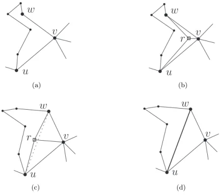
At this point we have two consecutive edges uv and vw of the facial walk so that edgeuw can be added to the graph while preserving the planarity of the graph, as in Figure1(a). We will morph drawings Γ1 and Γ2 so that edge uw can be added as a straight-line segment preserving
planarity. (In case our facial walk bounds an inner face that contains no disconnected components, we could have chosen uw to be an ear of a triangulation of the face in one of the drawings, thus avoiding the need to morph that drawing; but in the general case we must morph both drawings.) The argument is the same for both drawings, so we describe it only for Γ1. Vertices u and w are
consecutive neighbors of v. Add a new neighbor r of v between u and w in cyclic order, and add edgesrv,ru, and rw. It is possible to placer close enough to vinΓ1 so that the resulting drawing
is straight-line planar and (v, r, u) and (v, r, w) are faces. See Figure1(b)for an example.
u
w
v
(a)
r
u
w
v
(b)
u
w
v
r
(c)
u
w
v
(d)
Figure 1: Morphing to add edge uw. (a) Verticesu, v and w are consecutive around a facial walk, and the graph does not currently contain the edgeuw. (b) A vertexr is added suitably close tov and connected tov,u, and w. (c) After convexifying the quadrilateralurwv. (d)Vertexr and its incident edges can be removed in order to insert edge uw.
Figure 1(c). To do this, we temporarily triangulate the drawing1 and then apply Quadrilateral Convexification to urwv.
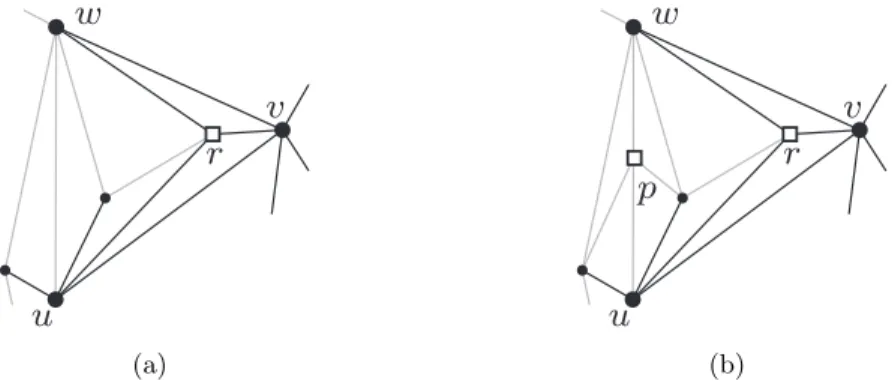
There is one slight complication: it might happen that when we triangulate the drawing, we add the edge uw, which would make it impossible to convexify the quadrilateral urwv. In this case, we remove uw and retriangulate the resulting quadrilateral by adding a new vertex p placed at any internal point of line segment uw, and adding straight-line edges fromp to the four vertices of the quadrilateral. See Figure2.
u w
v r
(a)
u w
v r p
(b)
Figure 2: If edge uw has been added when triangulating the drawing (a), then we subdivide uw with the insertion of a vertexp and we triangulate the two facesp is incident to (b).
After convexifying the quadrilateral urwv, we remove the temporary triangulation edges, remove r, and add the edge uw. See Figure1(d).
Thus with two calls to Quadrilateral Convexification (one for each drawing), we have added one edge to both drawings. Moreover, the two drawings are still topologically equivalent drawings of the same planar graph. We can continue until every facial cycle of every connected component (except an isolated vertex or edge) is a triangle. Since planar graphs have O(n) edges, in total we useO(n) calls to Quadrilateral Convexification.
Part B. At this point every connected component is either an edge, a vertex, or a triangulation. We will now morph and add edges to connect the components together. Once all of the components have been connected we will again appeal to Part A to triangulate the full connected graph.
Consider a face that has c0 connected components drawn inside it. The outer boundary of the face is a triangle abc, and each inner component is either a single vertex or edge, or is bounded by a triangle. The high-level idea is to shrink all of the inner components so that there is freedom to move them around within abc. We will use this freedom to line up the inner components in the same order in both drawings, starting from a position near a. It will then be straightforward to connect the outer component with the first inner component via an edge from aand add edges between consecutive inner components to connect the rest.
In order to determine the size to which we must shrink the inner components, it will be helpful to have triangular boundaries for each inner component (even for the ones that are single vertices or edges) that are disjoint, lie within abc, and have positive area.
1
a
b
c
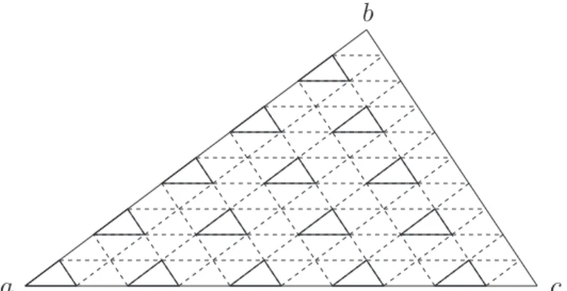
Figure 3: Roads (bounded by dashed lines) and homes (small solid triangles) within triangular face abc.
To this end, consider each inner component that is a vertexu. In each drawing a sufficiently small disk centered atucontains no part of the drawing other than vertexuitself. Then a positive-area triangle formed by vertex u and two new “dummy" vertices can be inserted in the disk to become the triangular boundary for that component. Similarly, consider each inner component that is an edge uv. In each drawing a sufficiently thin rectangle having uv as a side contains no part of the drawing other than edge uv itself. Then a positive-area triangle formed by edge uv and a new “dummy” vertex can be inserted in the rectangle to become the triangular boundary for that component.
Now, consider a uniform triangular grid such thatalies on a vertex of the grid and each grid cell is either a homothetic copy ofabc (called anupward cell) or a homothetic copy of the triangle obtained by rotating abc by π radians (called a downward cell). Let every second row of cells in any of the three directions determined by the sides ofabcbe a road. Let any cell that is not in any road be a home. We fix the parities of the rows such that the upward cell adjacent to ainabcis a home. Note that all homes are thus upward cells. See Figure 3. We have yet to specify the size of a grid cell. We require a grid size such that the following conditions are satisfied: 1) there are at leastc0 homes alongacand 2) each bounding triangle of an inner component contains a home.
For each inner component, let itshome region be the largest homothetic copy of an upward cell that can be inscribed in the component’s triangular boundary. Let d be the diameter of abc. We can, for example, set the grid size such that the diameter of a grid cell is the minimum of: 1) d/(2c0) and 2) a fifth of the diameter of the smallest home region. If the diameter of a grid cell is at most the first value, then there must be at least 2c0 upward cells along ac, half of which are homes. If the diameter of a grid cell is at most the second value, then every home region is at least five times the size of an upward cell. Every home region of this size must contain a home. In fact, every home region of this size contains a homothetic copy ofabcwhose side lengths are three times the side lengths of an upward cell; further, at least one of the six upward cells contained in this homothetic copy ofabc is a home.
Consider an inner component bounded by triangle uvwwith a home region that contains a homeh. We choose a non-dummy vertex ofuvwand call it the component’sconnector. Our goal is to morph the inner component intohsuch that its connector is near the vertex ofhthat is farthest
u
v
w
Figure 4: Movements of the connector of uvw used to shrink and rotate uvw into h. The solid triangles are, from outermost to innermost: uvw, the home region ofuvw, the final position ofuvw within h. The dashed triangle is the midpoint polygon of the home region ofuvw.
a
c
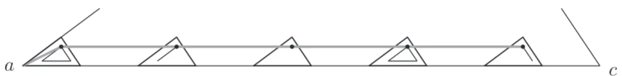
Figure 5: Edges (thick grey lines) linking the connectors (dots) of the inner components that lie in the homes alongac.
from ac. We will do so with O(1) morphs of uvw via linear movements of single vertices of uvw, during which the contents of uvw move along linearly. By Lemma 3, these are each unidirectional morphs.
We first morphuvwto occupy exactly the component’s home region with a linear movement of each vertex. We then rotate the positions of the vertices of uvw so that the connector is in the position farthest from ac. This can be done with six linear movements of the vertices, using the home region’s midpoint polygon as an intermediate. Finally, with a linear movement of each vertex, we shrinkuvwintoh such that uvwbecomes a slightly smaller homothetic copy of hand does not intersect the boundary of h. There is no interference between inner components since uvwremains in its original bounding triangle for the duration of the morph. See Figure 4. Observe that we performed O(1)unidirectional morphs for each of thec0−1 connected components.
We can now arrange the c0 inner components in any arbitrary order in the homes along edgeac using c0 home swaps. Since all of the inner components are in homes, the road network is unimpeded and the roads are wide enough to allow passage of any inner component. By navigating along the road network, it is straightforward to swap the homes of two inner components using O(1) linear movements of the components. Thus, in O(c0) unidirectional morphs, we can arrange the inner components into the homes alongacin the same order in both drawings. Finally we add edges between the connectors of adjacent components and add an edge from ato the connector of the first component and we are done connecting the components. See Figure 5.
Once all components are connected, we remove all dummy vertices and edges and appeal to part A to triangulate the full connected graph. This completes the description of part B.
Altogether, we useO(c)unidirectional morphs to connect theccomponents of the graph. We also addO(n) edges in Part A, and each addition takes two calls to Quadrilateral Convexification. Furthermore, each call to Quadrilateral Convexification usesO(1)unidirectional morphing steps by Theorem 6. Therefore, in total we use O(n) unidirectional morphing steps.
We now analyze the running time of the algorithm. We call Quadrilateral Convexification O(n) times, and each call takesO(n2) time. This dominates the other work done by the algorithm (e.g. we find O(n) temporary triangulations, each of which takes O(nlogn) time). Thus the total running time isO(n3).
5 Morphing Between Two Triangulations
In this section we prove our main result, Theorem 1, for the case of triangulations. Since the previous section reduced the general case to the case of triangulations, this will complete the proof of Theorem1.
Theorem 9. Let Γ1 and Γ2 be two triangulations that are topologically equivalent drawings of an
n-vertex maximal planar graph G. There is a morph from Γ1 to Γ2 that is composed of O(n)
unidirectional morphs. More precisely, the morph uses O(n) unidirectional morphs plus O(n) calls to Quadrilateral Convexification. Furthermore, the morph can be constructed in O(n3) time.
As described in Subsection1.1, our approach is to find an internal vertexvof degree at most five and then morph the drawings using O(1)unidirectional morphs so thatv can be contracted to the same neighbor u in both drawings. We will prove a time bound of O(n2) for this step. More details are given below.
After this step, we contract v to u in both drawings and apply recursion to find a morph M between the two smaller triangulations. The result is a pseudomorph: we contract v to u in
Γ1, apply M, and then reverse the contraction of v to u in Γ2. The number of steps satisfies
the recurrence relation S(n) = S(n−1) +O(1), which solves to S(n) ∈ O(n). Finally, we apply Theorem7to convert the pseudomorph to a morph with the same number of unidirectional morphs. Each appeal to Theorem7takes timeO(n) since that is the bound on the number of unidirectional morphs. Thus the total time bound is given by the recurrence relation T(n) =T(n−1) +O(n2),
which solves to T(n)∈O(n3).
We now fill in the details about finding vertex v and contracting it to a common neighbor in both drawings. If there are no internal vertices, then we only have the outer triangle and a unidirectional morph with O(1) morphing steps is easily computed in time O(1). Otherwise, we claim that there is an internal vertexvof degree at most 5. To see this, note that the triangulation has 3n−6 edges, and thus the sum of the degrees is 6n−12. Every vertex has degree at least 3, and if all the internal vertices had degree at least 6, the sum of the degrees would be at least
3(3) + 6(n−3) = 6n−9.
Ifv has degree 3 then we can contractv to the same neighbor u in both drawings. Ifv has degree 4 or 5 then letu be a neighbor ofv to whichv can be contracted in Γ2. (The existence ofu
is guaranteed by applying Lemma 4 to the polygon ∆(v) inΓ2.) If v can be contracted to u inΓ1
we are done. Otherwise, we will morphΓ1 to make this possible. Note that there are no external
chords fromuto any vertex of∆(v), because the two drawings are topologically equivalent, andΓ2
has no such chords.
Ifvhas degree 4 then the neighbors ofvmust form a non-convex quadrilateralQwith vertices abcd, where d, say, is the reflex vertex. We contractv todand apply Quadrilateral Convexification toQ, noting that the quadrilateral has no external chords. Specifically, there is no chordacbecause v cannot be contracted to u, so u must be one of a, c, and, as noted above, there are no external chords incident to u. After convexification, we movev slightly into the interior of∆(v) to obtain a drawing in which vertexv can be contracted tou. The result is a pseudo-morph, which we convert to a morph using Theorem 7. The number of unidirectional steps is O(1) and the time bound is O(n2) by Theorem6.
Ifv has degree 5 then the neighbors of v form a pentagonabcdewhere we want to contract v to u = a, say. We use a similar method, morphing the pentagon until it is “almost” convex by making a few calls to Quadrilateral Convexification. More formally:
Lemma 10. Let Γ be an n-vertex triangulation. Suppose v is a non-boundary vertex of degree 5, with neighbors forming a pentagonabcde, and suppose thatais not incident to any external chords of the pentagon. Then we can morphΓ, keeping the outer boundary fixed, so thatvcan be contracted to a. The morph consists of at most two calls to Quadrilateral Convexification plus a constant number of unidirectional morphing steps. Furthermore, the morph can be found in O(n2) time.
Proof. Because v’s neighbors form a pentagon, v can be contracted to some neighbor x while preserving planarity (Lemma4). Ifx=awe are done, so suppose they are different. Contract v to x. We will divide into two cases depending on whether x is adjacent toaon the pentagon or not.
First consider the case wherexis not adjacent toa. Without loss of generality, suppose that x = c. See Figure 6(a). We use Quadrilateral Convexification to convexify acde. This is possible since ceis an inner chord andad is not an external chord. Nowasees all the quadrilateralacdeas well as the triangle abc. Thusv can now be contracted to a.
a
b
c
d
e
(a)
a
b
c
d
e
(b)
Figure 6: (a) Vertexv has been contracted to x =cand we wish to contract v to a. (b)Vertexv has been contracted tox=band we wish to contractv to a.
Next consider the case where x is adjacent to a. Without loss of generality, suppose that x=b. See Figure6(b). Use Quadrilateral Convexification to convexifyabde. This is possible since beis an inner chord and ad is not an external chord. Now dsees all the quadrilateral abdeas well
as the triangle bcd. Move vertex vin a straight line from x=b to d. This puts us in the first case. We use Theorem 7to convert the resulting pseudomorph to a morph.
The morph consists of at most two calls to Quadrilateral Convexification plus a constant number of unidirectional morphing steps. The morph can be found in O(n2) time.
6 Quadrilateral Convexication
In this section we give an algorithm for Problem5, to morph a triangulation in order to convexify a quadrilateral. The main result of the section is as follows:
Reminder of Theorem 6.Quadrilateral Convexification can be solved via a single unidirectional morph. Furthermore, such a morph can be found in O(n2) time.
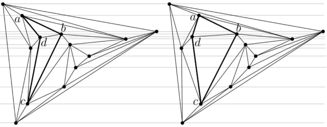
In the rest of this section we will prove Theorem 6. Recall that we have an n-vertex tri-angulation Γ and a quadrilateral abcd in Γ with no vertex inside it and such that neither ac nor bdis an edge outside of abcd. Our goal is to morph Γ so that abcd becomes convex using a single unidirectional morph.
We first describe the main idea. Ifabcdis convex, then we are done. Assume without loss of generality thatdis the reflex vertex of the non-convex quadrilateral, i.e., the angle at dinternal to quadrilateralabcdis larger thanπ radians. This implies thatbis the tip of the arrowhead shape and that the triangulation contains the edgebd(see Figure7). Change the frame of reference so thatbd is “almost” horizontal. We will use one unidirectional morph that moves vertices along horizontal lines, i.e. preserving their y-coordinates. Our main tool will be a result about re-drawing a plane graph to have convex faces while keeping all vertices at the same y-coordinate—this is a result by Hong and Nagamochi [27] expressed in terms of level planar drawings of hierarchical graphs. To complete the proof we will show that the linear motion from the original drawing to the new drawing in fact preserves planarity, and therefore is a unidirectional morph.
d
b
a
c
Figure 7: Triangulation Γ, containing a non-convex quadrilateral abcd with a reflex vertex d, with no vertex inside it, with edgebdinside it, and with no chord outside it.
result. A hierarchical graph is a graph with vertices assigned to layers. More formally, ahierarchical graph is a triple (G, L, γ) such that G is a graph, L is a set of horizontal lines (sometimes called layers), and γ is a function mapping each vertex of G to a line in L in such a way that, if an edge (u, v) belongs to G, then γ(u)6= γ(v). (It is conventional to assume the layers are 1,2, . . . k, i.e., that successive horizontal lines are distance 1 apart, but that turns out to be unnecessary for Hong and Nagamochi’s result, as the fact that the horizontal lines are equally spaced is nowhere used in their proof.) With the lines in L ordered from bottom to top,γ represents a partial order on the vertices ofG, and we writeu≺γv if the line γ(u) is below the lineγ(v).
A level drawing of a hierarchical graph (G, L, γ) maps each vertex v of G to a point on the line γ(v) and each edge to a y-monotone curve. A level planar drawing is a level drawing in which no two curves representing edges cross; such a drawing is straight-line if edges are drawn as straight-line segments, andconvex if faces are delimited by convex polygons.
In our situation, we have a straight-line level planar drawing of a hierarchical graph and we want a straight-line convex level planar drawing that “respects” the embedding. More abstractly and more generally, Hong and Nagamochi define a hierarchical plane graph to be a hierarchical graph together with a combinatorial embedding (a rotation system and outer face) corresponding to some level planar drawing. In other words, a hierarchical plane graph is an equivalence class of drawings, and a drawing of a hierarchical plane graph must be a member of the equivalence class.
In order to guarantee a convex level planar drawing, Hong and Nagamochi require some conditions. Given a hierarchical plane graph(G, L, γ), anst-faceofGis a face delimited by two paths
(s=u1, u2, . . . , uk = t) and (s=v1, v2, . . . , vl =t) such that ui ≺γ ui+1, for every 1≤ i≤k−1,
and such that vi ≺γ vi+1, for every 1 ≤ i ≤ l−1. We say that (G, L, γ) is a hierarchical plane
st-graph if every face of Gis an st-face. Hong and Nagamochi give an algorithm that constructs a convex straight-line level planar drawing of any hierarchical plane st-graph [27]. Here we explicitly formulate a weaker version of their main theorem.2
Theorem 11. (Hong and Nagamochi [27]) Every 3-connected hierarchical plane st-graph(G, L, γ)
admits a convex straight-line level planar drawing.
We now proceed to prove Theorem 6 and hence to solve the Quadrilateral Convexification problem with a single unidirectional morph. First, we rotate the frame of reference so that edgebd is horizontal and then we rotate it a bit more, so that no two vertices have the samey-coordinate and so that the strip delimited by the horizontal lines through b and d contains no vertex of Γ, except for the presence of b and d on its boundary. Remove edge bd from Γ obtaining a planar straight-line drawing Γ0 of a planar graph G0. Draw a horizontal line through each vertex; let L be the set of these lines and let γ be the function that maps each vertex to the unique line in L through it; observe that, by the assumptions, γ represents a total order on the vertices of G0. We have the following.
Lemma 12. (G0, L, γ) is a 3-connected hierarchical plane st-graph.
2
We make some remarks. First, the result in [27] proves that a convex straight-line level planar drawing of(G, L, γ)
exists even if a convex polygon representing the cycle delimiting the outer face ofGis arbitrarily prescribed. More precisely, Hong and Nagamochi show a necessary and sufficient condition for a convex polygon (possibly with flat angles) to be the polygon delimiting the outer face of a convex straight-line level planar drawing of(G, L, γ). However, this condition is always satisfied if every internal angle of the polygon is convex. Second, the result holds for a super-class of the3-connected planar graphs, namely for all the graphs that admit a convex straight-line drawing [15,42].
Proof. By construction, Γ0 is a straight-line level planar drawing of (G0, L, γ), hence (G0, L, γ) is a hierarchical plane graph.
Further, every face ofG0is an st-face. This is trivially true for all faces delimited by triangles inΓ0, sinceγrepresents a total order on the vertices ofG. Moreover, this is true for the face delimited by abcd, since by the choice of the reference frame a is below both horizontal lines γ(b) and γ(d)
andcis above both of them, or vice versa. It follows that(G0, L, γ)is a hierarchical plane st-graph.
x=a b y=c
d
Figure 8: Illustration for the proof of Lemma12.
Finally, we prove that G0 is 3-connected. Refer to Figure 8. Suppose, for a contradiction, thatG0 is not3-connected. Then there exist two vertices xand ywhose removal from G0 results in a disconnected graphG00. Since Γ is3-connected, adding the edge bdto G00 reconnects this graph.
Therefore, b and d must be in different components of G00. Since G0 contains paths bad and bcd, it follows that {x, y} ={a, c}. Since removinga, c disconnectsG0, there is another face of G0 that contains aand c. This face is delimited by three edges (as the one delimited by quadrilateral abcd is the only face ofG0 which is not triangular), therefore contains the edge ac. However, this implies thatxy =acis a chord external to polygon abcd inΓ, thus contradicting the assumptions.
By Lemma 12, (G0, L, γ) is a 3-connected hierarchical plane st-graph. By Theorem 11, a convex straight-line level planar drawing Λ0 of (G0, L, γ) exists. In particular, polygon abcd is convex in Λ0. Construct a straight-line planar drawing Λ of G from Λ0 by drawing edge bd as an open straight-line segment. Due to the initial choice of the reference frame, this introduces no crossing in the drawing. To solve Problem Quadrilateral Convexification we use a single linear morph,hΓ,Λi, fromΓ intoΛ. See Figure9. We now prove the following lemma.
d
b
a
c
d
b
a
c
Lemma 13. The linear morphhΓ,Λi is planar and unidirectional.
Proof. The morph is certainly unidirectional, since each vertex is on the same horizontal line in the initial drawingΓ and the final drawing Λ. To prove planarity we will argue that no vertex crosses an edge during the motion. The tool we need is Lemma14, which proves that if two pointspandq each move at uniform speed along a horizontal line andq is to the right ofpin their initial and final positions, thenq is to the right ofp at every time instant. Lemma 14 will be stated and proved in Section7.2.1. Thus it suffices to show that for each horizontal line`inL, the left-to-right ordering of vertices lying on`and points where edges cross` is the same inΓ as inΛ. This follows directly from the fact that both drawings have the same faces, and every face is an st-face.
In order to complete the proof of Theorem 6, it remains to discuss the running time of the algorithm that solves Quadrilateral Convexification. Removing and re-inserting edgebdtakesO(1)
time. Other than that, we only need to apply Hong and Nagamochi’s algorithm, which takesO(n2)
time [27]. Thus the total running time isO(n2).
7 Converting a Pseudo-Morph to a Morph
In this section, we show how to convert a pseudomorph consisting of unidirectional morphing steps into a true morph of unidirectional morphing steps, assuming that the graph is triangulated and the vertices we contract have degree at most 5. Specifically, we prove the following.
Reminder of Theorem 7. Let Γ1 and Γ2 be two triangulations that are topologically equivalent
drawings of an n-vertex maximal planar graph G. Suppose that there is a pseudomorph fromΓ1 to
Γ2 in which we contract an internal vertex v of degree at most 5, performk unidirectional morphs,
and then uncontractv. Then there is a morphMfromΓ1 toΓ2 that consists of k+ 2 unidirectional
morphs. Furthermore, given the sequence of k+ 1 drawings that define the pseudomorph, we can modify them to obtain the sequence of drawings that define Min O(k+n) time.
Suppose that the given pseudo-morph consists of the contraction of an internal vertexvwith deg(v)≤5 to a vertexa, followed by a morph M0 =hΓ1, . . . ,Γk+1iof the reduced graph, and then
the uncontraction of v from a. Suppose that hΓi,Γi+1i is an Li-directional morph, for 1≤ i≤k. We assume that the drawings Γ1, . . . ,Γk+1 are given to us, and show how to update the sequence
of drawings to those of Min timeO(n+k).
Specifically, we will show how to addv and its incident edges back into each drawing of the morph M0 keeping each step unidirectional. We will preserve planarity by placing v at an interior point of the kernel of∆(v). Call the resulting morphM00. We will perform the modifications from M0 to M00 in time O(k). To obtain the final morph M, we replace the original contraction of v to a by a unidirectional morph that moves v from its initial position to its position at the start of M00, then follow the steps of M00, and then replace the uncontraction of v by a unidirectional morph that moves v from its position at the end of M00 to its final position. The result is a true morph that consists ofk+ 2unidirectional morphing steps. It takesO(n) time to add the two extra unidirectional morphs to the sequence, since we must add two drawings of an n-vertex graph.
Thus our main task is to modify the morph M0 by adding vertex v and its incident edges back into each drawing of the morph sequence in constant time per drawing, preserving planarity and maintaining the property that each step of the morph sequence is unidirectional. We can ignore everything outside the polygonP = ∆(v). Note that vertexaremains in the kernel ofP throughout the morph. We distinguish cases depending on the degree of v. Section 7.1proves Theorem 7 for the easy case where the degree ofvis 3 or 4. Section7.2proves Theorem7for the more complicated case wherev has degree 5.
7.1 Vertex v of Degree 3 or 4
In this section we prove Theorem 7 for the case where the contracted vertex v has degree 3 or 4, i.e.P is a triangle or quadrilateral. IfP is a triangle then by Lemma 3 we can place v at a fixed convex combination of the triangle vertices in all the drawingsΓi.
IfP is a quadrilateralabcd then the line segmentacstays in the kernel ofP because vertex a stays in the kernel of P. Thus, we can place v at a fixed convex combination of a and c in all the drawings Γi (using the degenerate version of Lemma 3 where the triangle collapses to a line segment).
The coordinates ofv in eachΓi can be computed in constant time, so the total time bound isO(k).
7.2 Vertex v of Degree 5
In this section we prove Theorem7for the case where the contracted vertexvhas degree 5. Our goal will be to place vertexvvery close to the vertexato which it was contracted in the pseudo-morph. LetP = ∆(v) be the pentagon abcdelabelled clockwise. We use the notation that b is at point bi in drawing Γi, etc.
We may assume that vertex a is fixed throughout the entire morph. This is not a loss of generality because if vertexamoves, we can translate the whole drawing to move it back: the morph in which every vertexv moveskv units along direction`¯is planar if and only if the morph in which every vertex moves kv −ka units along direction `¯is planar; and note that vertex astays fixed in the latter morph.
We want to place v within distance ε of a. We want ε small enough so that at any time instanttduring morphhΓ1, . . . ,Γk+1ithe intersection between the diskDcentered atawith radius
ε and the kernel of polygon P consists of a positive-area sector S of D. Since the morph consists of k linear morphs, we can compute a value forεas follows. For 1≤i≤k letεi be the minimum during the unidirectional morph hΓi,Γi+1i of the distance fromato any of the edgesbc, cd, de. We
claim thatεi can be computed in constant time on our real RAM model of computation. It suffices to compute the minimum distance betweenaand each of the three infinite lines throughbc, cd,and de. This is because we can test if the minimum occurs inside the relevant line segment, and we can compute the minimum distance from ato each of the moving endpointsb, c, d, e. Consider the line through points p, q, where pq = bc, cd,or de, and points p and q each move on parallel lines at uniform speed during the morph hΓi,Γi+1i. As a function of time, t, the square of the distance
t. We want to solve for the derivative being zero. The derivative has a cubic polynomial in the numerator, and a cubic equation can be solved in constant time on a real RAM model.
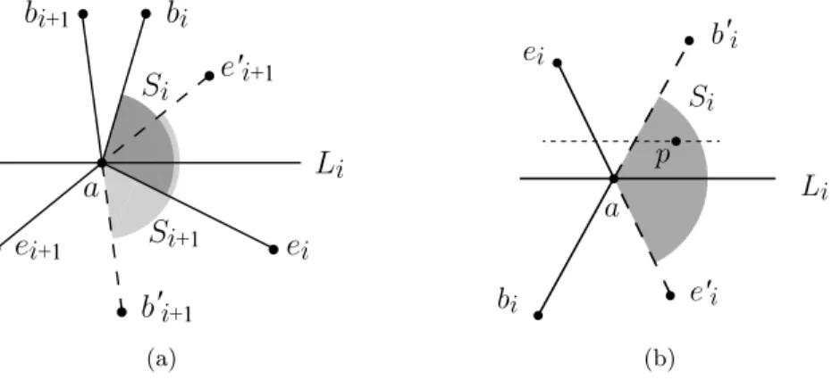
After computing each εi, let ε= min1≤i≤k{εi}. Thenεcan be computed in timeO(k). FixD to be the disk of radiusεcentered ata. In caseais a convex vertex of P, the sector S is bounded by the line segments aband ae and we call it apositive sector. See Figure 10(a). In caseais a reflex vertex of P, the sector S is bounded by the extensions of line segments aband ae and we call it a negative sector. See Figure 10(b). More precisely, let b0 and e0 be points so that a is the midpoint of the segments bb0 and ee0 respectively. The negative sector is bounded by the segmentsae0 and ab0. Note that when anL-directional morph is applied to P, the points b0 and e0 also move at uniform speed in directionL.
b
c e
D
a
d
S
(a)
D e
a b
c d
S
e' b'
(b)
Figure 10: A disk D centered at a whose intersection with the kernel of P (the lightly shaded polygonal region) is a non-zero-area sector S (darkly shaded). (a) Vertex a is convex and S is a positive sector. (b)Vertexais reflex and S is a negative sector.
The important property we use from now on is that any point in the sector S lies in the kernel of polygon P. This property immediately follows from the choice of ε. Let the sector in drawing Γi be Si, for i = 1, . . . , k+ 1. Recall our convention that hΓi,Γi+1i is an Li-directional morph.
Our task is to choose for each i a position vi for vertex v inside sector Si so that all the Li-directional morphs keep v inside the sector at all times. We will separate the proof into two parts. One part is to show that there exist pointsvi inSi so that the line segmentvivi+1 is parallel
to Li. This is in Section 7.2.2. The other part of the proof is to show that such points vi ensure thatv is inside sector S throughout the morph. This is in Section 7.2.1.
For both proofs, we will distinguish the following two possibilities for the relationship be-tweenSi and the lineLi translated to go through pointa.
One-sided case. Pointsbi and ei lie in the same closed half-plane determined byLi. In this case, whether the sectorSi is positive or negative,Li does not intersect the interior ofSi. See Figure11. AnLi-directional morph keepsbi andei on the same side ofLiso ifSi is positive it remains positive and if Si is negative it remains negative. Observe that v remains inside the sector if and only if it remains inside Dand between the two lines abandae.
bi
ei
a Si
Li
ei+1
bi+1
Si+1
(a)
bi ei
a Si
Li
p
(b)
Figure 11: The one-sided case whereSi lies to one side ofLi, illustrated for a positive sectorSi. (a) An Li-directional morph toSi+1. (b)v remains inside the sector if and only if it remains insideD
and between the two linesaband ae.
of the sectorSi. See Figure 12. During anLi-directional morph the sectorSi may remain positive, or it may remain negative, or it may switch between the two, although it can only switch once. Observe that v remains inside the sector if and only if it remains insideDand on the same side of the linesbb0 andee0.
bi
ei
a Si
Li
ei+1 bi+1
Si+1 b'i+1
e'i+1
(a)
bi
ei
a
Si
Li
p b'i
e'i
(b)
Figure 12: The two-sided case where Si contains points on both sides of Li. (a)An Li-directional morph from the positive sectorSibounded bybiaeito the negative sectorSi+1bounded bye0i+1ab0i+1.
(b)v remains inside the sector if and only if it remains inside Dand on the same side of the lines bb0 andee0.
7.2.1 Sectors and the betweenness property
In this subsection we show that if we can choose points vi in sector Si such that the linevivi+1 is
parallel to Li thenv remains inside the sector throughout the morph.
Our main tool is the following lemma proving that “sidedness” on lineL is preserved in an L-directional morph.
Lemma 14. Let L be a horizontal line and p0, p1, q0, q1 be points in L. Consider a point p that
is a point that moves at constant speed from q0 to q1 in one unit of time, then q is to the right of p
during their entire movement. Note that p0 may lie to the right or left of p1 and likewise forq0 and
q1.
L
p0 q0 p1 q1
Figure 13: Pointsp and q move fromp0 to p1 and fromq0 to q1 respectively.
Proof. Letpi andqi,i= 0,1, be points as described above, see Figure 13. Denote bypt andqtthe positions ofp andq, for 0≤t≤1. First note that
qi =pi+δi (1)
for i= 0,1, withδi >0. Since p andq are moving at constant speed, we havept= (1−t)p0+tp1
and qt= (1−t)q0+tq1. Now, using equation (1) in the expression forqt we have qt= (1−t)(p0+δ0) +t(p1+δ1)
=pt+ (1−t)δ0+tδ1,
where(1−t)δ0+tδ1 >0.
Clearly, Lemma 14 generalizes to a directed line L that is not necessarily horizontal, if we interpret “to the right of” as “further in the direction of” L.
Corollary 15. Consider an L-directional morph acting on points p, r ands. Ifp is to the right of the line through rsat the beginning and the end of theL-directional morph, thenp is to the right of the line through rsthroughout the L-directional morph.
To prove Corollary15, consider a lineL0 throughpthat is parallel toLand apply Lemma14 to points pand q, whereq is the intersection of L0 and the line through r and s.
We now present our main result about the relative positions of points vi and vi+1.
Lemma 16. If point vi lies in sector Si and point vi+1 lies in sector Si+1 and the line segment
vivi+1 is parallel to Li then an Li-directional morph from Si, vi to Si+1, vi+1 keeps the point in the
sector at all times.
Proof. First consider the one-sided case. Suppose Si is a positive sector (the case of a negative sector is similar). Observe that v remains in the sector during anLi-directional morph if and only if it remains in the disk D and remains between the lines ab and ae. See Figure11(b). Because vi and vi+1 both lie in D, the line segment between them also lies in the disk, and v remains in
D throughout the morph. In the initial configuration,vi lies between the lines abi and aei, and in the final configuration vi+1 lies between the lines abi+1 and aei+1. Therefore, by Corollary 15, v
remains between the lines throughout the Li-directional morph. Thus v remains inside the sector throughout the morph.
Now consider the two-sided case. Observe that a point v remains in the sector during an Li-directional morph if and only if it remains on the same side of the lines bb0 and ee0. Note that
this is true even when the sector changes between positive and negative, since the points inS are those in Dthat are between lines bb0 and ee0. See Figure cionzo12(b). As in the one-sided case,v
remains in the disk throughout the morph. Also, v is on the same side of the lines bb0 and ee0 in the initial and final configurations, and therefore by Corollary15,vremains on the same side of the lines throughout the morph. Thusv remains inside the sector throughout the morph.
7.2.2 Nice points
In this subsection we prove that there exist points vi in Si such that the line segment vivi+1 is
parallel toLi. We call the possible positions forvi inside sector Si thenice points, defined formally as follows:
• All points in the interior ofSk+1 are nice.
• For1≤i≤k, a pointvi in the interior ofSi is nice if there is a nice pointvi+1 inSi+1 such
thatvivi+1 is parallel toLi.
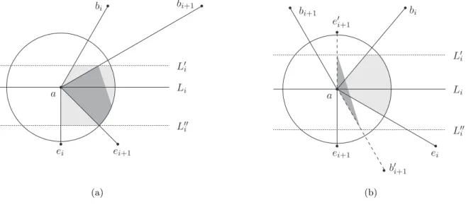
It suffices to show that all the sets of nice points are non-empty. We will in fact characterize the sets. Given a line L, an L-truncation of a sector S is the intersection of S with an open slab that is bounded by two lines parallel to Land contains a. Observe that this implies that the open slab will contain all points of S in a small neighborhood of a. In particular, an L-truncation of a sector is non-empty.
Lemma 17. The set of nice points in Si is anLi-truncation ofSi for i= 1, . . . , k.
Proof. LetNi denote the nice points in Si. The proof is by induction asigoes fromk+ 1to 1. All the points in the interior of Sk+1 are nice. Suppose by induction thatNi+1 is an Li+1-truncation
of Si+1.
Consider the one-sided case. See Figure 14. The slab determining Ni consists of all lines parallel to Li that go through a point of Ni+1. The slab is non-empty since Ni+1 contains all of
Si+1 in a small neighborhood of a. Thus the slab contains all points of Si in a neighborhood ofa, and thusNi is anLi-truncation of Si.
Consider the two-sided case. See Figure 15. The slab determining Ni consists of all lines parallel toLi that go through a point ofNi+1. The slab containsain its interior and thusNi is an Li-truncation of Si.
Lemma17 implies in particular that the set of nice points is non-empty.
The last thing we need to do to complete the proof of Theorem 7 for the case wherev has degree 5, is to show that the above procedure to compute thevi’s has a running time of O(k). It suffices to show how to compute Ni from Ni+1 in constant time. To do this, we just compute the
maximum and minimum points of Si+1 in the direction perpendicular to Li. The slab boundaries for Ni go through these points. ThenNi is the intersection of the slab with sectorSi.
Li ei
bi bi+1
ei+1
Li
a
Figure 14: Ni(lightly shaded) is anLi-truncation ofSiin the one-sided case. Ni+1 is darkly shaded.
The slab boundaries for Ni consist ofL0i and a parallel line just belowLi.
Li
ei
bi
ei+1
bi+1
Li
Li
a
(a)
Li
ei
bi
ei+1 e
i+1 bi+1
b
i+1
Li
Li
a
(b)
Figure 15: Ni(lightly shaded) is anLi-truncation ofSi in the two-sided case. Ni+1is darkly shaded.
L0i andL00i are the slab boundaries for Ni.
8 A Linear Lower Bound
In this section we prove Theorem2, that there exist two straight-line planar drawings of ann-vertex path such that any planar morph between them consists of Ω(n)linear morphs.
Specifically we will describe two straight-line planar drawings Γ and Λ of an n-vertex path P = (v1, . . . , vn), and prove that any straight-line planarity preserving morph M between Γ and Λ requires Ω(n) morphing steps. In order to simplify the description, we consider each edge ei = (vi, vi+1) as oriented fromvi to vi+1, for i= 1, . . . , n−1.
Drawing Γ (see Figure 16(a)) is such that all the vertices of P lie on a horizontal straight line with vi to the left ofvi+1, for each i= 1, . . . , n−1.
DrawingΛ (see Figure16(b)) is such that:
• for eachi= 1, . . . , n−1 withimod 3≡1,ei is horizontal with vi to the left ofvi+1;
• for each i= 1, . . . , n−1 with imod3 ≡2,ei is parallel to line y= tan(23π)x withvi to the right of vi+1; and
• for eachi= 1, . . . , n−1withimod 3≡0,ei is parallel to liney = tan(−23π)xwithvi to the right of vi+1.
v
1v
2v
3v
n(a)
v3
v2
v1
vn
(b) Figure 16: DrawingsΓ (a) and Λ (b).
LetM =hΓ = Γ1, . . . ,Γx = Λi be any planar morph transformingΓ intoΛ.
Fori= 1, . . . , n andj= 1, . . . , x, we denote byvij the point where vertex vi is placed inΓj and byeji the directed straight-line segment representing edgeei inΓj.
For 1 ≤ j ≤ x−1, we define the rotation ρji of ei around vi during the morphing step
hΓj,Γj+1i as follows (see Figure17). Translateei at any time instant of hΓj,Γj+1i so thatvi stays still during the entire morphing step. After this translation, the morph between eji and eji+1 is a rotation of ei around vi (where ei might vary its length during hΓj,Γj+1i) spanning an angle ρji.
We assumeρji >0if the rotation is counter-clockwise andρji <0otherwise. We have the following.
Lemma 18. For eachj = 1, . . . , x−1 andi= 1, . . . , n−1, we have |ρji|< π.
Proof. Assume, for a contradiction, that |ρji| ≥π, for some 1≤j≤x−1 and 1≤i≤n−1. Also assume, w.l.o.g., that the morphing step hΓj,Γj+1i happens between time instantst= 0and t= 1.
We introduce some notation. For any 0≤t≤1, we denote:
• by vi(t) the position ofvi at time instantt – note thatvi(0) =vij and vi(1) =vij+1;
• byvi+1(t)the position ofvi+1at time instantt– note thatvi+1(0) =vij+1andvi+1(1) =vij+1+1;