FHFA MORTGAGE ANALYTICS PLATFORM

(1)

DDRAFT

FHFA MORTGAGE

ANALYTICS

PLATFORM

Released by FHFA, July 10, 2014

Robert M. Dunsky

Xiaoming Zhou

Michael Kane

Ming Chow

Charles Hu

Andrew Varrieur

(2)

FHFA Mortgage Analytics Platform

1. BACKGROUND & INTRODUCTION... 2

2. FHFA MORTGAGE ANALYTICS PLATFORM OVERVIEW ... 3

3. PERFORMING LOAN MODULE ... 6

3.1 C

OMMON

I

NDEPENDENT

V

ARIABLES IN THE

P

ERFORMING

L

OAN

M

ODULE

... 7

3.2 S

PECIAL

T

REATMENT OF

P

ERFORMING

M

ODIFIED

L

OANS

... 12

4. NON-PERFORMING LOAN MODULE ... 15

4.1 I

NDEPENDENT

V

ARIABLES IN THE

N

ON

-P

ERFORMING

L

OAN

M

ODULE

... 16

5. CREDIT LOSS MODULE

... 19

5.1 C

HARGE

-O

FF

T

IMING

... 20

5.2 C

HARGE

-O

FF

A

MOUNT

... 20

5.3 REO

O

PERATIONS

E

XPENSES

... 25

6. INTEGRATION MODULE

... 27

6.1 S

CHEDULED AND

U

NSCHEDULED

R

ELATED

P

RINCIPAL

... 27

6.2 C

REDIT

L

OSS

R

ELATED

P

RINCIPAL

... 28

6.3 C

REDIT

L

OSS

M

EASURES

... 28

7. STANDARDIZED REPORT ELEMENTS ... 30

8. REFERENCES ... 32

9. APPENDIX A: SPLINE CONSTRUCTION... 33

10. APPENDIX B: PERFORMING LOAN MODULE MODEL COEFFICIENTS ... 34

11. APPENDIX C: BACK-TESTING PLOTS ... 51

12. APPENDIX D: NON-PERFORMING LOAN EQUATION PARAMETERS... 65

(3)

FHFA Mortgage Analytics Platform

1. Background & Introduction

The Federal Housing Finance Agency (FHFA) maintains a proprietary Mortgage

Analytics Platform to support the Agency’s strategic plan. The objective of this white

paper is to provide interested stakeholders with a detailed description of the platform,

as it is one of the tools the FHFA uses in policy analysis. The distribution of this white

paper is part of a larger effort to increase transparency on mortgage performance and

the analytical tools used for policy analysis and evaluation within the FHFA.

The motivation to build the FHFA Mortgage Analytics Platform derived from the

Agency’s need for an independent empirical view on multiple policy initiatives.

Academic empirical studies may suffer from a lack of high quality data, while empirical

work from inside the industry typically represents a specific view. The FHFA

maintains several vendor platforms from which an independent view is possible, yet

these platforms tend to be inflexible and opaque. The unique role of the FHFA as

regulator and conservator necessitated platform flexibility and transparency to carry

out its responsibilities.

The FHFA Mortgage Analytics Platform is maintained on a continuous basis; as such,

the material herein represents the platform as of the publication date of this document.

As resources permit, this document will be updated to reflect enhancements to the

platform.

(4)

FHFA Mortgage Analytics Platform

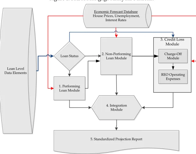
2. FHFA Mortgage Analytics Platform Overview

The platform integrates econometric loan performance models, loan level data and

external economic forecasts to project mortgage cash flows. This section offers an

overview of the modules and their interconnections.

Economic Forecast Database

House Prices, Unemployment,

Interest Rates

Loan Level

Data Elements

Loan Status

1. Performing

Loan Module

2. Non-Performing

Loan Module

Charge-Off

Module

4. Integration

Module

5. Standardized Projection Report

Figure 1: FHFA Mortgage Analytics Platform

REO Operating

Expenses

3. Credit Loss

Module

There are two sources of external inputs to the analytics platform: loan level data and

economic forecasts. The economic forecasts include projections of house prices, interest

rates and unemployment rates through the forecast horizon. Both vendor-supplied

economic forecasts and FHFA projections of economic variables are stored in the

(5)

FHFA Mortgage Analytics Platform

economic forecast database. These economic forecasts cover a wide range of economic

environments from baseline to highly optimistic to extremely stressful economic

conditions. The economic forecast databases are quarterly.

The loan level data elements are the second source of external inputs; these include

approximately thirty variables per loan comprising loan attributes and borrower

characteristics. The platform projects mortgage performance from the loan’s current

age to termination, including foreclosure alternatives and the resolution of real estate

owned (REO). The platform applies projected probabilities of termination to

performing loan balances such that a portion of the loan prepays, becomes delinquent

and may resolve as a default each month. To simplify the discussion within this paper,

when a loan is said to prepay (or default), only a portion of the loan is prepaying (or

defaulting), not the whole loan. The components of the platform are summarized

below and are described in greater detail in subsequent sections of this paper.

1. Performing Loan Module – the primary function of this module is to project

monthly loan level prepayment and 90-day delinquency probabilities on performing

and modified performing loans. Loans enter into this module if they are current, less

than 90 days delinquent, or forecasted to cure from a delinquency during the

simulation. The prepayment and delinquency equations are functions of borrower

characteristics, loan characteristics, home values and other economic variables.

Multiple pairs of prepayment and delinquency equations collectively cover several loan

products and modified loans guaranteed or owned by the Enterprises.

2. Non-Performing Loan Module – the primary function of this module is to project

lifetime outcomes for delinquent loans. Loans enter into this module if they are 90 to

180 days delinquent at the beginning of the projection, or if they are predicted to

become delinquent within the performing loan module. The module outputs four

mutually exclusive loan-specific probabilities each month: foreclosure completion

(REO), voluntary prepayment, foreclosure alternative resolutions and re-performance

(cure). The foreclosure alternative resolutions include deed-in-lieu of foreclosure,

pre-foreclosure sale (short sale), and third party sale. A loan is defined as re-performing

when all arrearages are paid and the cure is not due to a modification or restructuring.

The models are a function of borrower characteristics, house prices and state legal

structures. Unlike the performing loan module where multiple product level models

are constructed, only one set of equations is estimated for non-performing loans.

(6)

FHFA Mortgage Analytics Platform

3. Credit Loss Module– the primary function of this module is to calculate loan

level credit losses and determine the appropriate timing of loss recognition. Loans

enter into this module if they are greater than 180 days delinquent at the start of the

projection or are projected to generate a credit loss from the non-performing module.

Credit losses are measured as charge-offs and REO operating expenses. Charge-offs

and REO operating expenses are calculated at the loan level using an accounting

approach.

4. The Integration Module - combines the forecasted performance elements,

mortgage contractual terms, and interest rates to generate loan level cash flows. This

module outputs are aggregated across loans into the Standardized Projection Report.

5. The Standardized Projection Report –summarizes projections of portfolio

performance measures over the forecast horizon. Key credit loss elements reported in

the report are charge-offs and REO operation expenses. Other variables in the report

include performing balances, dollars of new 90 day delinquencies, scheduled and

unscheduled principal payments, guarantee fee income, and credit enhancement claims.

The subsequent sections of the paper discuss each of the modules in detail. Sections 3

through 5 focus on the design of the econometric behavioral equations, Section 6

reviews the credit loss calculations, and Section 7 covers the calculation of the monthly

projections. The appendices include the parameter estimates and back testing results

from the modules covered in Sections 3 through 5.

(7)

FHFA Mortgage Analytics Platform

3. Performing Loan Module

The Performing Loan Module contains a series of Multinomial Logit (MNL) equations

that predict the loan’s monthly status: current, prepaid or delinquent. Many authors

including Clapp et al (2005) and Jenkins (1995) demonstrate that the MNL provides a

convenient method for structuring prepayment and delinquency risk as a discrete-time

competing hazard. Using the estimated equation parameters, the platform calculates

the conditional probability of prepayment and 90-day delinquency as,

(

)

(

) (

)













+

=

90 , , , ,

_ˆ

'

exp

ˆ

'

exp

1 ˆ

'

exp

)

(

f t i pp t i pp t i t i

v

x

prepay

P

β

, and

(

)

(

)

(

)













+

=

90 , , 90 , ,

_ˆ

'

exp

ˆ

'

exp

1 ˆ

'

exp

)

90 (

f t i pp t i f t i t i

v

x

v

f

P

β

.

The probability of remaining current is calculated as,

)

(

)

90 (

1 )

(

current

i,t

P

f

i,t

P

prepay

i,t

P

=

−

.

Where

β

ˆ

pp

and

β

ˆ

f90

represent the estimated prepayment and 90-day delinquency

parameter vectors, while

x

i,t

and

v

i,t

represent the variables in the prepayment and

delinquency equations for the

ith

loan at time period

t

. The resulting prepayment

probability represents the likelihood that loans will prepay in the current month, given

that it has neither prepaid nor become 90 days delinquent in the prior month. The

delinquency probability is similarly defined.

Fifteen loan product specific models are estimated using historical loan-level data in

addition to a single model for all modified loans. The treatment of performing

modified loans is discussed in detail in Section 3.2. The loan product models are based

on the following eight products:

Fixed Rate Products: 40yr. FRM, 30yr. FRM, 20yr. FRM, 15yr. FRM

Adjustable Rate Products: 10/1 ARM, 7/1 ARM, 5/1 ARM, 3/1 ARM,

(8)

FHFA Mortgage Analytics Platform

Separate loan product models are estimated for each Enterprise, with the exception of

the fixed rate 40 year loan product and modified loans, which are estimated with data

combined from both Enterprises due to the low volume of fixed rate 40 year loan

product and modified loans. When possible, the entire historical population of loans is

used for estimation. In the case of the fixed rate 30 year loans, a stratified proportional

sample of three million loans is selected for each Enterprise. The stratification variables

include: geography, credit scores, origination quarter, property type, loan size, original

loan to value (LTV) and occupancy. The marginal distributions of the population and

the selected samples are compared to ensure representativeness to the loan population.

These eight loan products for each GSE represent approximately 99 percent of the

Enterprise mortgages originated since 1995. The remaining loans are comprised mostly

of single family balloon mortgages and step rate mortgages. These loans are assigned

to the product model based on their maturity term, for example, a 30 year step rate

mortgage is assigned to the 30 year fixed rate model.

3.1 Common Independent Variables in the Performing Loan Module

This section reviews the common independent variables across all of the estimated

behavioral equations for performing loans. Most of the continuous explanatory

variables are constructed as spline functions, with the locations of the spline knots

varying across models

1 _{. The parameter estimates, standardized errors, and the}

locations of spline knots are listed in Appendix B. Back-testing plots of each model is

located in Appendix C.

3.1.1 Loan Seasoning

The loan age, or seasoning, is included in the models to capture changes in the

delinquency and prepayment tendencies over the life of the loan. The seasoning

functions in the models are constructed as a set of age spline variables; the spline knots

1

_{The spline specification for continuous independent variables is a common practice in prepayment and default modeling (see}

Dunsky and Ho (2007), Bajari, Chu, and Park (2008), Tracey Seslen and William C. Wheaton (2010)). An important benefit of the

spline specification is that it avoids sudden jumps within a continuous variable while allows for the non-linearity relationship

between independent and dependent variable.

Page 7

(9)

FHFA Mortgage Analytics Platform

are chosen from the product specific hazard curve(s) that best represents the product

loan population

2 _.

3.1.2 Vintage-Fixed Effects

In lieu of a constant term, each model is estimated with a series of vintage-specific fixed

effects. The estimated fixed effects capture unobservable changes in underwriting

standards and other non-observables that are not controlled for elsewhere in the model.

3.1.3 Seasonality

All of the models include a set of eleven monthly indicators (dummy variables) to

capture seasonality. Seasonality is a common phenomenon in mortgage performance:

prepayments during the summer months are typically borrowers moving, while late

payments frequently occur in April. The estimated seasonality parameters measure

sensitivity of prepayment and delinquency relative to January, the omitted month.

3.1.4 Down Payment at Origination

Down payment is measured in terms of the original loan-to-value (LTV) ratio; loan size

is the balance of the loan at origination and value is the appraised value at origination.

Underwriting requirements typically predetermine loan down payments. Enterprise

loans require a minimum original LTV of 80 on first lien mortgages, or, if the down

payment is less than 20 percent, then a form of credit enhancement is required, (e.g.

mortgage insurance) . The original LTV enters the model as a set of spline variables,

where the spline knots are selected at approximately the 20

th

_{, 40}

th

_{and 80}

th

_{percentiles of}

original LTV in the estimation data.

3.1.5 Credit Score at Origination

The Enterprises fully adopted credit scores in their underwriting criteria in the

mid-1990s. Nearly 100 percent of loans originated since 1995 in the estimation data contain

credit scores. Credit scores are typically reported from all three of the credit

repositories. The model only uses one credit score per loan. When multiple scores are

available per borrower, the model uses the lower of the two scores if two are reported,

and the middle score if three scores are reported. The lowest score across all borrowers

is used when co-borrowers are reported in the loan data. Credit scores are specified as

2

_{The historical hazards are plotted from the loan populations even when sampling is required.}

Page 8

(10)

FHFA Mortgage Analytics Platform

five spline variables; the spline knots are selected based on the distribution of credit

scores in the estimation data.

3.1.6 Spread at Origination (SATO)

The SATO variable captures the difference between the borrower’s mortgage rate and

the prevailing interest rate reported in the Primary Mortgage Market Survey (PMMS)

on the date of the origination. Historically, this spread measures the borrower’s price of

credit relative to the market average. To the extent that borrower credit is priced

imperfectly, the SATO measure captures other unobservable in the transaction. There

are two SATO spline variables (two spline segments, one spline knot) in each model.

The spline knot is located at the median value of the difference between the initial rate

on the mortgage and the market rate (PMMS rate) in the month of the first payment.

3.1.7 Loan Size at Origination

Loan size (in thousands) is an important factor in the prepayment equation; the value of

refinancing a loan is proportional to the size of the loan. For some mortgage products,

loan size is also inversely related to the incidence of delinquency. The loan size at

origination enters the specification as a series of four spline variables; the spline knots

are selected based on the distribution of loan size in the estimation data sets.

3.1.8 Time Varying Credit-Equity Function (Credit Score Current-LTV Interaction)

The credit equity function is the interaction between the original credit score group

indicator and spline variables of the current LTV (or mark-to-market LTV, MTM LTV)

over the observed life of the loan, similar to Lam et al [2013]

3 _{. The function enables}

measuring the borrower’s responsiveness to changes in current LTV while controlling

for the borrower’s original credit score.

There are (k) groups of credit score indicators; each borrower’s score falls uniquely into

one of the five buckets (

k=5

). The width of each bucket is based on the distribution

observed in the estimation data. The time dependent MTM LTV ratio is expanded into

(

h

) spline variables. The length and locations of the spline segments are defined from

the estimation data. The credit equity function in compact format for the

i

th

_{loan in}

period

t

is defined as

3

_{LTVs are updated in the simulation model via house price indexes from the economic forecast database. The FHFA state-level}

purchase-only index is used for both model estimation and forecasting.

Page 9

(11)

FHFA Mortgage Analytics Platform

∑∑

= =

=

5 1 5 1 , , , , ,

,

ˆ

_

h k h t i k t i k h t

i

Credit

Score

MTM

LTV

Equity

Credit

β

.

Where

Credit

_

Score

i,t,k

takes the value of zero or one, depending on the loan’s credit

score, and

MTM

_

LTV

i,t,h

are a series of spline variables based on the current LTV of the

loan. For each combination of credit score groups (

k=1 to 5

) and MTM LTV range (

h=1

to 5

) a

β

ˆ

h,k

parameter is estimated.

The above table displays credit equity function parameter estimates (not marginal

effects) from the delinquency equation for a 30 fixed rate product model. The table is

included here only to demonstrate that the estimated parameter values vary across the

MTM LTV spline variables for a given credit score group. A loan remains in one credit

score group throughout the simulation yet moves left and right in the table as the loan

MTM LTV changes during the simulation. The benefit of the credit equity function is

that the marginal change in the probability of delinquency is not assumed to be

constant across credit score groups or over the MTM LTV spline variables.

3.1.9 Time Varying Refinance Burnout Function

The refinance function is constructed to capture the sensitivity of borrower prepayment

behavior to changes in market interest rates, similar to Dunsky & Ho [2007]. The

refinance function is specified as the interaction between a refinance ratio and a burnout

factor. The burnout factor captures the difference in the refinancing efficiency between

two otherwise identical loans that have gone through different historical interest rate

experiences.

Credit Score

Group

0 to 60 60 to 70 70 to 85 85 to 95 95 to 120

350 to 682

2.921

1.335

1.816

3.463

0.913 682 to 720

2.154

3.384

3.989

3.078

1.444 720 to 750

1.921

4.088

4.650

4.096

1.755 750 to 780

1.485

5.424

5.109

5.571

2.011 780 to 850

1.307

5.306

5.025

6.961

2.125 MTM LTV Spline Variables

Estimated Credit Equity Parameters

(12)

FHFA Mortgage Analytics Platform

The refinance function is defined as

t i t

i t

i

refinance

ratio

burnout

function

refinance

_

,

=

_

,

*

,

, where













=

= t i t i t i

PMMS

ratio

refinance

, 0 , ,

_

The refinance ratio is constructed as the ratio of the Primary Mortgage Market Survey

(PMMS) rate for the ith loan at origination (t=0) to the current period PMMS rate. The

PMMS rate is the current mortgage rate at time t. The refinance ratio is a pure

macroeconomic measure of the value of the refinance option and devoid of borrower

specific credit information; this is in contrast to the spread at origination variable

(SATO). The burnout factor is defined in terms of the significantly positive refinance

spread cumulated over the age of the mortgage, reflecting missed refinance

opportunities. Explicitly the burnout function is defined as,

∑

= =













−

=

T

t it

t i t i t i

PMMS

MAX

burnout

0 , , 0 ,

,

0 .

1 ,

0 .

We assume that a refinance opportunity occurs whenever the prevailing PMMS rate

falls below the PMMS rate at origination by 10 percent.

The refinance burnout function should have the qualitative behavior of an S curve,

which typically represents the refinance incentive as a function of interest rates; when

the refinance –ratio is low, there is a constant base refinancing rate. As the refinance

ratio increases, the refinancing rate also increases. But when the refinance-ratio exceeds

a certain level, the refinancing rate should remain stable, at a high level. However, the

behavior of this

S

function varies with the burnout level. The refinance function

estimates multiple

S

functions as we categorize the loans into five buckets by the

burnout function. The burnout refinance function is only included in the prepayment

equations for the fixed rate products.

(13)

FHFA Mortgage Analytics Platform

3.1.10 State Unemployment Rate

The unemployment rate serves as a proxy for job loss of the borrower as well as to

capture local economic activity. Although prepayment is generally insensitive to the

unemployment rate, the delinquency rate increases with the unemployment rate. There

are four unemployment spline variables in each model. The selection of the spline

knots is based on the distribution of the unemployment rate of the states represented in

the input data.

3.1.11 Yield Curve Spread at Origination

The yield curve spread, measured by the difference between the 2-year and the 10-year

swap rate, captures the slope of the swap curve and serves as a proxy for the state of the

macro-economy. In the absence of large scale monetary intervention, empirical

evidence suggests an upward sloping yield curve presents a healthy macro-economic

environment. Existing borrowers would be expected to respond to a flattening of the

yield curve when long term rates decline as a refinance opportunity. Alternatively,

when the yield curve inverts, although refinance opportunities may persist,

delinquencies typically increase reflecting a weaker macro-economic environment.

Yield curve spread is only included in the prepayment equation.

Parameter estimates, spline knots and back testing results of models discussed in the

Performing Loan Module are located in Appendices B and C.

3.2 Special Treatment of Performing Modified Loans

Performing modified loans include loans that have been modified through Home

Affordable Modification Program (HAMP) or the Enterprises’ proprietary modification

programs and have not re-defaulted (90+ days delinquent). Performing modified loans

are treated differently from unmodified performing loans. Modified loans, most of

which were seriously delinquent before modification, have a higher likelihood of

delinquency than unmodified performing loans. Modification of the mortgage terms

(mortgage rate, amortization term and principal forbearance) and the delinquency

status prior to modification are important variables in projecting the prepayment and

re-default behaviors. A single prepayment and re-default model is developed and

deployed for all modified loans.

The behavioral equations for modified loans are modeled in the same multinomial logit

framework as unmodified performing loans described above. While most of the

(14)

FHFA Mortgage Analytics Platform

independent variables and all the economic variables used in the performing loan

model are retained in the modified loan model, some independent variables are

reconstructed. The reconstructed variables include loan age, seasonality, loan size and

the refinance spread. Loan age for modified loans is measured from the modification

date, and loan size is the post modification loan balance. Seasonality is captured by a

quarterly dummy variable instead of a monthly dummy due to the short performance

history of modified loans. The refinance spread is defined as the modified interest rate

of the mortgage minus the prevailing mortgage rate and is constructed as a spline

variable.

The independent variables for the performing loan behavioral equations that are not

retained in the modified loans treatment are original vintage, original down payment,

SATO and the credit equity function. Vintage is not considered for the modified loans

treatment as most modified Enterprises loans were modified after 2009, and the

underwriting environment has not changed significantly from 2009 to 2012. Down

payment and SATO are also not retained as these two variables are not meaning given

that loan has been modified. Finally, the credit equity function is excluded to maintain

a relatively simple structure for the modified loan equations.

Additional independent variables are added to the behavioral equations for modified

loans:

Percentage Change in the Monthly Mortgage Payment:

The monthly payment on most

modified loans is reduced through interest rate reductions, term extensions or principal

forbearance. The monthly payment reduction represents a financial relief to the

distressed mortgage borrower and should reduce the borrower’s tendency to default on

the loan. The percentage change in the monthly mortgage payment is constructed as a

spline variable with the knots determined by the selected percentiles of the distribution

of the monthly payment percentage change.

Delinquency Status prior to Modification:

Deeply delinquent borrowers face a greater

financial challenge than less delinquent borrowers to bring the payment status of the

loan back to current. Deeply delinquent borrowers also have less flexibility to prepay

the loan due to the large financial obligation of accrued or capitalized interest. The

Delinquency Status prior to Modification is constructed as linear spline variables with

knots at 3, 6 and 12 month delinquency.

(15)

FHFA Mortgage Analytics Platform

Home Price Appreciation since Modification:

Home Price Appreciation since

Modification is measured as a percentage change of the home price since modification

at the state level. A positive home price appreciation indicates an improved borrower’s

equity position in the property, and should reduce the borrower’s probability to

re-default on the mortgage. Home Price Appreciation is measured at the state level and is

constructed as linear spline variables with knots determined by selected percentiles of

the distribution of the percentage of the home price change.

The behavioral equations are estimated with performance history on Fannie Mae and

Freddie Mac loans from June 2009 to December 2011. The estimated coefficients and

back-testing results for the Modified Loan equations are included in Appendices B and

C.

(16)

FHFA Mortgage Analytics Platform

4. Non-Performing Loan Module

Loans enter into the non-performing module if they are 90 to 180 days delinquent at the

beginning of the projection or if they are predicted to become 90-days or more

delinquent (F90) during the forecast horizon. The module computes four mutually

exclusive lifetime probabilities conditional on a loan being at least 90 days delinquent:

re-performance (cure), voluntary prepayment, alternative foreclosure resolution, and

foreclosure completion (REO). The lifetime probability of the loan resolving as real

estate owned (REO) is calculated as the residual of one minus the other three computed

probabilities. The alternative foreclosure resolutions include deed-in-lieu of

foreclosure, pre-foreclosure sale, and third party sale. Re-performance is defined as a

loan returning to current status without having been modified or restructured. The

loans that are projected to be re-performing are treated as performing loans and are sent

back to the Performing Loan Module.

The equations in the non-performing module are estimated simultaneously on a

population of loans that became 90 days delinquent for the first time between 1997 and

2012. The estimation data excludes loans that became 90 or more days delinquent and

were subsequently modified. Conceptually, the resolution of delinquent loans is jointly

determined by the borrower and the servicer. Information on servicers is unobservable;

therefore the equations are a function of borrower, house characteristics and state legal

structures. The lifetime probability of each of the terminal states is represented below in

a competing risks framework:

(

)

(

)

(

)

(

)













+

=

PP t i RPerf t i FCA t i FCA t i t i t i

v

x

f

le

LifetimeSa

P

β

ω

β

ˆ

'

exp

ˆ

'

exp

ˆ

'

exp

1 ˆ

'

exp

)

90 |

(

, , , , , ,

(

)

(

) (

)













+

=

PP t i RPerf t i FCA t i RPerf t i t i t i

v

x

v

f

RPerf

P

β

ω

β

ˆ

'

exp

ˆ

'

exp

ˆ

'

exp

1 ˆ

'

exp

)

90 |

(

, , , , , ,

Page 15

(17)

FHFA Mortgage Analytics Platform

(

)

(

)

(

)

(

)



_









+

=

PP t i RPerf t i FCA t i PP t i t i t i

v

x

f

epay

Pr

lifetime

P

β

ω

β

ω

ˆ

'

exp

ˆ

'

exp

ˆ

'

exp

1 ˆ

'

exp

)

90 |

(

, , , , ,

,

, and

)

90 |

(

)

90 |

(

)

90 |

(

1 )

90 |

(

LifetimeRE

O

i,t

f

i,t

P

LifetimeSa

le

i,t

f

i,t

P

RPerf

i,t

f

i,t

P

Lifetime

Pr

epay

i,t

f

i,t

P

=

−

.

Where

β

ˆ

FCA

,

β

ˆ

RPerf

and

β

ˆ

PP

represent the equation specific parameters of exiting by a

foreclosure alternative, re-performance and voluntary prepayment of the mortgage.

The corresponding independent variable vectors are

x

i,t

,

v

i,t

and

ω

i,t

for the

ith

loan at

the time of the 90 day delinquency event, time

t

.

The following subsection discusses the construction of the independent variables in the

model.

4.1 Independent Variables in the Non-Performing Loan Module

There are seven groups of independent variables in the non-performing loan model,

and an intercept term. Similar to the performing modified loan model, only one model

is deployed for all non-performing loans. Consideration of explanatory variables is

restricted to variables that are observable in the month of the first 90 day delinquency

and for which economic forecasts are available.

4.1.1 Current LTV at the Delinquency Date

In order to capture the level of equity or negative equity in the property, the current

LTV (MTM LTV) of the loan in the month of the first 90 day delinquency is included as

five spline variables. The spline knots are located at 68%, 82%, 99% and 120% current

LTV. MTM LTV is calculated from the loan balance on the last paid installment, and

house values are updated using the FHFA state-level purchase-only House Price Index.

4.1.2 Original Loan Size

Similar to the performing loan module, original loan size (in thousands) is included in

the model by five spline variables with knot locations based on the distribution of loan

size in the delinquent loan data. The spline knots are located at $90k, $150k, $232k, and

$360k.

(18)

FHFA Mortgage Analytics Platform

4.1.3 Property Type

The property type is represented by three indicator variables; condominium, planned

urban development and manufactured housing. Single family detached residence

serves as the comparator.

4.1.4 Stated Occupancy at Origination

To differentiate between outcomes across owner occupants and non-owner occupants

an indicator variable is included in all of the specifications. Relative to owner

occupants, non-owner occupants are less likely to re-perform.

4.1.5 Mortgage Insurance Coverage

For loans with mortgage insurance, two spline variables based on the level of insurance

coverage are included in the specification. The spline knot is located at 25% coverage.

The spline variables for loan without mortgage insurance are set at zero.

4.1.6 Credit Score at Origination

Original credit scores enter into the model as five spline variables with spline knots

located at 623, 661, 703, and 750. Original credit scores may no longer accurately

represent the borrower’s recent payment history, yet they remain statistically significant

in the non-performing loan model.

4.1.7 State Unemployment at Delinquency Date

Four unemployment spline variables are included in each model where the selection of

the spline knots is based on the distribution of the unemployment rate of the states

represented in the input data. The spline knots are located at 5.5, 7.8, and 10.3 percent.

4.1.8 Judicial State Indicator

Lastly, a state legal structure indicator is included to control for variation in state

foreclosure laws. The judicial state indicator is set to 1 when the loans is located in the

following states: DE, FL, HI, IA, ID, IL, IN, KS, KY, LA, ND, NE, NJ, NM, NY, OH, OK,

PA, SC, and SD. In judicial foreclosure states, a lender is required to get a judgment

against the borrower and a court order authorizing the sale of the property by an office

of the court, (Hayre and Saraf, 2008). The foreclosure timelines in judicial states are

longer than non-judicial states. As such, it is necessary to control for the local legal

structures when modeling delinquent loan outcomes.

(19)

FHFA Mortgage Analytics Platform

The estimated parameters for the equations of the non-performing loan module are

provided in Appendix D.

(20)

FHFA Mortgage Analytics Platform

5. Credit Loss Module

The Credit Loss Module projects credit losses on loan balances that are 180+ days

delinquent at the beginning of the projection period, and on loan balances that are

projected to go to either foreclosure completion (i.e., REO) or to a

foreclosure-alternative sale from the Non-Performing Loan Module. The platform projects two

accounting measures of loss;

Charge-off

and

REO Operating Expenses

.

6/1/2014 - 6/8/2014

Foreclosure Expense Period

Foreclosure Time Line

Charge-off

Foreclosure expenses are accumulated

until the property title transfer date and

recognized as a off. The

charge-off amount equals the sum of expected

net REO sale proceeds, paid expenses,

3 months of paid interest, and minus

the MI Claim.

REO Time Line

REO Operating Expenses are recognized

monthly and continue until the property

is sold. REO Operating Expenses includes

paid expenses and monthly declines in

the REO property value.

An REO appreciation

adjustment is recognized at on

the REO Sale Date

6/1/2014 - 6/8/2014

REO Expense Period

REO Sale

Date

Title Transfer

Date

LPI

Date

Figure 2: Charge-offs & REO Operating Expenses

Charge-off Recognition

REO Operations Expense Recognition

Figure 2 schematically separates the differences between Charge-offs and REO

operating expenses over the delinquency and resolution lifecycle. Expense components

included in the charge-off measure are accumulated from the borrower’s last paid

installment (LPI) date to the date of the title transfer. Two forms of title transfers

generate credit losses; foreclosure completions and alternative foreclosure resolutions.

Loans that complete the foreclosure process and become real estate owned (REO) are

charged off at the title transfer date (orange arrow) and begin to generate REO

(21)

FHFA Mortgage Analytics Platform

operating expenses thereafter. Meanwhile, loans that terminate via an alternative

foreclosure resolution are charged off at the title transfer date (orange arrow); these

loans do not become REO and therefore do not generate REO operating expenses. The

calculation of charge-offs for both forms of title transfer are identical, while only

completed foreclosures generate losses captured in REO operating expense.

In contrast to charge-offs, where expenses are accumulated over the foreclosure period

and recognized on the title transfer date (orange arrow), REO Operating Expenses are

calculated and recognized monthly (blue arrows). The sections below discuss the

specifics of the recognition timing, charge-offs amounts, and REO Operations Expenses.

5.1 Charge-Off Timing

Non-performing loans are charged off when the property title is transferred at the

completion of the foreclosure process or at the culmination of an alternative foreclosure

resolution

4 _{. The title-transfer timelines are calculated from historical data as the}

average number of months to complete the process in each state. The platform includes

both a long run timeline and a stressed foreclosure timeline. The stressed timeline

represents the average foreclosure timeline for loans that completed the foreclosure

process (or alternative foreclosure resolution) during the December 2010 to December

2011 period. The long-run average timelines are calculated from foreclosures (and

alternatives) completed from January 1995 to December 2011.

Non-performing loans with a level of delinquency greater than the historical state

average foreclosure timelines require a special treatment. These loans are assumed to

complete foreclosure (or an alternative foreclosure resolution) and be charged off

during the first 12 months of the projection. To avoid concentrating all of the

charge-offs in a particular month, each of these loans were randomly assigned a charge-off date

(based on a uniform distribution) during the first year of the projection.

5.2 Charge-Off Amount

The charge-off amount represents the expected proceeds from the property sale net of

all transaction costs, accrued expenses and credit enhancements.

𝐶ℎ𝑎𝑟𝑔𝑒𝑂𝑓𝑓

=

𝐸𝑥𝑝𝑒𝑐𝑡𝑒𝑑

𝑁𝑒𝑡

𝑅𝐸𝑂

𝑆𝑎𝑙𝑒

𝑃𝑟𝑜𝑐𝑒𝑒𝑑𝑠

4

_{Alternative foreclosure resolutions include deed-in-lieu of foreclosure, pre-foreclosure sale, and third party sales.}

Page 20

(22)

FHFA Mortgage Analytics Platform

+

𝑃𝑎𝑖𝑑

𝐸𝑥𝑝𝑒𝑛𝑠𝑒𝑠

+

𝑃𝑎𝑖𝑑

𝐼𝑛𝑡𝑒𝑟𝑒𝑠𝑡 − 𝑀𝐼

𝐶𝑙𝑎𝑖𝑚

𝐴𝑚𝑜𝑢𝑛𝑡

More specifically, the charge-off amount is composed of four components: (1) Expected

Net REO Sale Proceeds, (2) Paid Expenses during the Foreclosure Process, (3) Three

Months of Lost Interest, and (4) the Mortgage Insurance Claim Amount. Each of these

elements is discussed below.

5.2.1 Expected Net REO Sale Proceeds

The expected net REO sale proceeds are calculated as,

𝐸𝑥𝑝𝑒𝑐𝑡𝑒𝑑

𝑁𝑒𝑡

𝑅𝐸𝑂

𝑆𝑎𝑙𝑒

𝑃𝑟𝑜𝑐𝑒𝑒𝑑𝑠

=

�𝑈𝑃𝐵 ∗

(1 +

𝐹𝐶

𝐶𝑜𝑠𝑡𝑠

)

� − �𝑅𝑒𝑜𝑆𝑎𝑙𝑒𝑃𝑟𝑖𝑐𝑒

𝑡+𝑘

∗

(1

− 𝑆𝑒𝑡𝑡𝑙𝑒𝑚𝑒𝑛𝑡

)

�

where

�𝑈𝑃𝐵 ∗

(1 +

𝐹𝐶

𝑐𝑜𝑠𝑡𝑠

)

�

represents the unpaid principal balance (UPB) scaled up by

the foreclosure cost factor

(1 +

𝐹𝐶

𝑐𝑜𝑠𝑡𝑠

)

. The foreclosure cost factor is adapted from the

Home Affordable Modification Program Net Present Value (HAMP NPV) model’s

state-level averages of “Foreclosure and REO costs” as a percentage of UPB

5 _{. The NPV}

model documentation indicates that these costs are comprised of the following.

• Attorney and trustee fees

• Possessory and eviction fees and expenses

• Bankruptcy expenses

• Servicer liquidation expenses

• MI premium

• Flood insurance premium

• Title insurance

• Appraisal fees

• Property inspection

• Utilities

• Property maintenance/preservation

• Other foreclosure and holding costs

• Total repairs (capped at $3,000 to exclude discretionary repairs)

• Participation expenses

• Foreclosure costs paid out at property sale (from HUD-1)

These items combine both foreclosure costs (which belong in charge-off) and REO costs

(which do not belong in charge-off). To balance out the inclusion of REO cost elements,

5

_{The HAMP model documentation is available at,}

https://www.hmpadmin.com//portal/programs/docs/hamp_servicer/npvmodeldocumentationv502.pdf

Page 21

(23)

FHFA Mortgage Analytics Platform

the “Foreclosure and REO costs” are reduced by half when calculating the charge-off

amount. The remaining half is allocated to REO operations expense in Section 5.3.2.

The second part of expected net REO sale proceeds

�𝑅𝑒𝑜𝑆𝑎𝑙𝑒𝑃𝑟𝑖𝑐𝑒

𝑡+𝑘

∗

(1

− 𝑆𝑒𝑡𝑡𝑙𝑒𝑚𝑒𝑛𝑡

)

�

captures the expected revenue from the sale of the REO property net of brokerage fees

and other settlement costs. REO sales price, denoted as

𝑅𝑒𝑜𝑆𝑎𝑙𝑒𝑃𝑟𝑖𝑐𝑒

𝑡+𝑘

, represents the

expected value at time period

t

given a foreclosure timeline of

k

months. REO property

typically sells at a depressed price relative to a non-distressed transaction. The REO

sale price is calculated in two steps to account for the distressed nature of REO

property.

1. The original value of the property is “marked forward” by the percentage change

in the FHFA state-level purchase-only house price index between loan

origination and charge-off date.

2. The “marked forward” value of the house is haircut by a state-level REO stigma

correction.

While many REO sales are cash transactions

6 _{, the FHFA state-level purchase-only house}

price index includes a very small percentage of REO purchase transactions. Therefore,

it is necessary to adjust the REO property value in step 1 above by a state-level REO

stigma. The REO stigma correction maps the relationship between FHFA state-level

purchase-only house price index-based home values to distressed REO sales prices.

REO stigma correction follows a modified version of the approach used in the HAMP

Net Present Value (NPV) model

7 _{. In contrast to the HAMP NPV model, where REO}

Sale prices are regressed on home values generated by an automated valuation model

(AVM), the AVM prices are replaced by the property values in step 1 above (home

values generated from the FHFA state-level purchase-only home price). An REO

stigma equation is estimated for each of the 50 states based on Enterprise data. For all

alternative foreclosure resolutions, it is assumed that there is no REO stigma.

6

_{See for example,}

http://www.corelogic.com/blog/authors/molly-boesel/2014/05/cash-sales-made-up-40-percent-of-total-home-sales-in-february.aspx?WT.mc_id=crlg_140519_oBvIb&elq=a1f819d883a44c33952168e917f41adc#.U3osDfldV8E

Page 22

(24)

FHFA Mortgage Analytics Platform

The REO Sales price is reduced by settlement costs

(1

− 𝑆𝑒𝑡𝑡𝑙𝑒𝑚𝑒𝑛𝑡

)

as a percentage of

the calculated REO disposition sale price, the percentage varies by state. The state-level

settlement cost percentages are from the HAMP NPV model.

Settlement Charges include:

• Discount Points

• Loan Origination Fees

• Broker’s Bonus

• Broker Commission Fees

• Buyer’s Closing Costs (paid by seller only—not total buyer’s closing

• costs)

• Title Fee Cost

• Seller’s Closing Costs

• Assessments

• FHA/VA Non-Allowable Costs

• Other Costs

• Wire Fees

• Subtract miscellaneous revenues received at property sale:

o

Per diem amount

o

Other rent/interest amount

o

Prepaid interest amount

5.2.2 Paid Expenses during the Foreclosure Process

There are three groups of expenses that are accumulated from the last paid installment

to the foreclosure completion (or alternative foreclosure resolution) date: property

taxes, property insurance, and maintenance costs. Lookup tables containing the three

average expense rates are calculated from American Community Survey (ACS 2010) by

location and property value. Apart from homeowners’ association fees or

condominium fees, maintenance costs on single family homes are not reported in ACS.

As a proxy for monthly maintenance cost on single family homes, it is assumed that the

property maintenance costs are equal to one half homeowners’ association fees that

would have been applied if the home belonged to a homeowners’ association.

The expense rates are applied to the property value at loan origination and by

geographic state to project these monthly expenses in dollars. The monthly expenses

(25)

FHFA Mortgage Analytics Platform

are accumulated for every month between LPI date and foreclosure completion date

and recognized on the charge-off date.

5.2.3 Paid Interest

The module assumes that the loan servicer advances the borrower’s interest payment to

investors for three months, and this amount is reimbursed to the loan servicer by the

Enterprise when the loan is purchased out of the security. Three months of interest

payments are included as an expense in the charge-off amount.

5.2.4 MI Claim Amount

For loans with active MI coverage, the MI claim amount is limited to the insured UPB

plus foreclosure expenses. Foreclosure expenses are equal to the expenses in charge-off

plus lost interest for all months from the LPI date to foreclosure completion date. As

noted in 5.2.3 above, only three months of lost interest is included in the charge-off

measure.

The model assumes that the MI Company will exercise their right to buy the foreclosed

property (conveyance) in lieu of paying the MI Claim when the MI payment is greater

than the sum of the charge-off and REO operating expenses. In the case of conveyance,

the value of the property is based on the FHFA state-level purchase-only house price

index at the foreclosure completion date, not at the projected REO sale date. Both the

charge-off and REO net expenses attributed to the Enterprise are zero when the MI

Company purchases the foreclosed property.

For loans with original LTV greater than 80% and with first pay date on or later than

July 29, 1999, that coverage is projected to cancel at the earlier of: (a) the month after the

loan’s amortization LTV reaches 78 percent, and (b) the month in which the loan’s age

reaches one half its amortization term.

8 _{For loans originated before July 29, 1999 where}

the data indicate that MI coverage is in effect at the beginning of the projection, the

coverage is never canceled.

The calculated MI claim, whether or not the property conveys, is subject to the risk that

the MI Company either fails to meet its obligations (e.g. State regulator places the

8

_{See 12 U.S. Code § 4902 - Termination of private mortgage insurance regarding the “automatic” and “final” termination}

provisions of section 3 of the Homeowners Protection Act of 1998. There is no projection of the borrower-initiated cancellation

allowable under the Act.

Page 24

(26)

FHFA Mortgage Analytics Platform

company into runoff), or the MI company denies the claims. To allow for these forms of

counter party credit risk, the Module reduces the value of the calculated MI benefit by a

“haircut” percentage. When the platform is run to measure counterparty exposures the

haircut is assumed to be zero, yet when the platform is run to project GSE credit losses

the haircut ranges between 20 and 25 percent.

For alternative foreclosure resolutions, mortgage insurance is applied in the same way

as it is with foreclosed loans. The conveyance calculation is identical to the one used for

foreclosure, based on the idea that the MI would not make any payment beyond that

which would reduce the Enterprise’s loss to zero.

5.3 REO Operations Expenses

5.3.1 REO Operation Expense Timing

REO operation expenses are calculated and reported one month after foreclosure

completion until the REO property is sold. Similar to the foreclosure timings, the

platform includes both a long run REO timeline and a stressful timeline. The stressed

timeline represents the average state-level timelines for REO properties that were sold

between December 2010 and December 2011. The long-run average timelines are

calculated from REO sales completed from January 1995 to December 2011. Both sets of

REO sale time lines are computed from GSE historical data at the state level.

5.3.2 REO Operation Expense Amount

REO operations expenses are posted monthly and calculated as the sum of (1) paid

expenses and (2) mark-to-market REO property value changes. The REO expenses are

the same as the expenses included in the charge-off amount; “Paid Expenses” described

in Section 5.2.2 and the remaining 50% of the “Foreclosure and REO costs” allocated

across the REO holding period. In contrast to the expenses in the charge-off amount,

REO operating expenses are recognized each month while the property is held in

inventory.

Mark-to-market REO property values enter into the REO operations expense amount in

two parts. During the REO holding period, only declines in the value of the REO

property are added to the monthly REO operations expenses. Increases in the REO

property value are only included in the REO operating expenses when the property is

(27)

FHFA Mortgage Analytics Platform

sold. The mark-to-market property values are computed using projected FHFA

state-level purchase-only house price index.

As noted above, if the calculated charge-off excluding the estimated MI payment is

negative, both the charge-off and the REO operations expenses that would have been

associated with the loan termination are set to zero. It is explicitly assumed that

foreclosed or alternative foreclosures cannot generate gains. The best outcome for a

non-performing loan is a zero credit loss.

(28)

FHFA Mortgage Analytics Platform

6. Integration Module

This module integrates the prepayment and default probabilities from the Performing

and Non-performing Modules with the outputs from the Credit Loss Module to project

monthly loan-level cash flows. The primary outputs include scheduled and

unscheduled principal payments, scheduled interest payments, and losses. Ancillary

outputs include servicing fees, guaranty fee revenue, and MI payments.

For each mortgage, the unpaid principal balance is projected forward one month by

subtracting expected amounts of scheduled, prepaid (unscheduled), and defaulted

principal from the performing balance (

𝑈𝑃𝐵

𝑡−1

)

.

𝑈𝑃𝐵

𝑡+1

=

𝑈𝑃𝐵

𝑡−1

− 𝑠𝑐ℎ𝑒𝑑𝑃𝑟𝑖𝑛𝑃𝑎𝑖𝑑

𝑡

− 𝑝𝑟𝑒𝑝𝑎𝑦𝐷𝑜𝑙𝑙𝑎𝑟𝑠

𝑡

− 𝑑𝑜𝑙𝑙𝑎𝑟𝑠𝐹

90 𝑇𝑜𝑃𝑟𝑒𝑝𝑎𝑦

𝑡

−

𝑑𝑜𝑙𝑙𝑎𝑟𝑠𝐹

90 𝑇𝑜𝑅𝑒𝑜

𝑡

− 𝑑𝑜𝑙𝑙𝑎𝑟𝑠𝐹

90 𝑇𝑜𝑆𝑎𝑙𝑒

𝑡

.

For expository purposes the above equation is separated into two parts, (1) scheduled

and unscheduled principal, and (2) elements that are subtracted from performing

balance that are directed to the credit losses

(

𝑑𝑜𝑙𝑙𝑎𝑟𝑠𝐹

90 𝑇𝑜𝑅𝑒𝑜

𝑡

,

𝑎𝑛𝑑

𝑑𝑜𝑙𝑙𝑎𝑟𝑠𝐹

90 𝑇𝑜𝑆𝑎𝑙𝑒

𝑡

)

.

6.1 Scheduled and Unscheduled Related Principal

The scheduled and unscheduled principal payments include scheduled paid principal

(schedPrinPaid

t

) net lifetime losses, unscheduled or prepaid principal (

prepayDollars

t

)

from performing balances, and unscheduled or prepaid principal from delinquent loans

balances (

dollarsF90toPrepay

t

). More specifically, scheduled principal paid is defined as

𝑠𝑐ℎ𝑒𝑑𝑃𝑟𝑖𝑛𝑃𝑎𝑖𝑑

𝑡

=

𝑠𝑐ℎ𝑒𝑑𝑃𝑟𝑖𝑛

𝑡

∗

(1

− 𝑃

(

𝑙𝑖𝑓𝑒𝑡𝑖𝑚𝑒𝑅𝑒𝑜

𝑡

|

𝑓

90 𝑡

)

− 𝑃

(

𝑙𝑖𝑓𝑒𝑡𝑖𝑚𝑒𝑆𝑎𝑙𝑒

𝑡

|

𝑓

90 𝑡

))

.

And the remaining component

(1

− 𝑃

(

𝑙𝑖𝑓𝑒𝑡𝑖𝑚𝑒𝑅𝑒𝑜

𝑡

|

𝑓

90 𝑡

)

− 𝑃

(

𝑙𝑖𝑓𝑒𝑡𝑖𝑚𝑒𝑆𝑎𝑙𝑒

𝑡

|

𝑓

90 𝑡

))

represents the portion of the balance related to foreclosure and foreclosure-alternative

as described in the Non-Performing Module, Section 4.

Prepaid dollars on performing loan balances (

prepayDollars

t

) is defined as

𝑝𝑟𝑒𝑝𝑎𝑦𝐷𝑜𝑙𝑙𝑎𝑟𝑠

𝑡

=

𝑃

(

𝑝𝑟𝑒𝑝𝑎𝑦

𝑡

)

∗

(

𝑈𝑃𝐵

𝑡−1

− 𝑠𝑐ℎ𝑒𝑑𝑃𝑟𝑖𝑛

𝑡

)

,

(29)

FHFA Mortgage Analytics Platform

Where

𝑃

(

𝑝𝑟𝑒𝑝𝑎𝑦

𝑡

)

represents the probability of prepayment defined in Section 3,

Performing Loan Module. The second term in the prepaid dollars equation

(

𝑈𝑃𝐵

𝑡−1

−

𝑠𝑐ℎ𝑒𝑑𝑃𝑟𝑖𝑛

𝑡

)

, represent the loan balances at risk of prepaying not of their scheduled

principal payment.

The final source of prepaid dollars is from repayments on non-performing loans. There

are three components to

𝑑𝑜𝑙𝑙𝑎𝑟𝑠𝐹

90 𝑇𝑜𝑃𝑟𝑒𝑝𝑎𝑦

𝑡

: (1) the probability of going 90 days

delinquent from the performing loan module (Section 3), (2) the lifetime probability of

prepaying given that the balance is delinquent from the Non-Performing Module

(Section 4), and (3) the unpaid principal balance at risk.

𝑑𝑜𝑙𝑙𝑎𝑟𝑠𝐹

90 𝑇𝑜𝑃𝑟𝑒𝑝𝑎𝑦

𝑡

=

𝑃

(

𝑓

90 𝑡

)

∗ 𝑃

(

𝑙𝑖𝑓𝑒𝑡𝑖𝑚𝑒𝑃𝑟𝑒𝑝𝑎𝑦

𝑡

|

𝑓

90 𝑡

)

∗

(

𝑈𝑃𝐵

𝑡−1

− 𝑠𝑐ℎ𝑒𝑑𝑃𝑟𝑖𝑛

𝑡

)

6.2 Credit Loss Related Principal

Non-performing loan balances resolving as REO or an alternative foreclosure resolution

generate lost principal and contribute to the credit loss measures charge-off and REO

operating expenses. These two components of principal are subtracted from the

performing unpaid principal balance and represent the delinquent loan balances that

are later used to calculate charge-offs.

𝑑𝑜𝑙𝑙𝑎𝑟𝑠𝐹

90 𝑇𝑜𝑅𝑒𝑜

𝑡

=

𝑃

(

𝑓

90 𝑡

)

∗

𝑃

(

𝑙𝑖𝑓𝑒𝑡𝑖𝑚𝑒𝑅𝑒𝑜

𝑡

|

𝑓

90 𝑡

)

∗ 𝑈𝑃𝐵

𝑡−1

𝑑𝑜𝑙𝑙𝑎𝑟𝑠𝐹

90 𝑇𝑜𝑆𝑎𝑙𝑒

𝑡

=

𝑃

(

𝑓

90 𝑡

)

∗

𝑃

(

𝑙𝑖𝑓𝑒𝑡𝑖𝑚𝑒𝑆𝑎𝑙𝑒

𝑡

|

𝑓

90 𝑡

)

∗ 𝑈𝑃𝐵

𝑡−1

6.3 Credit Loss Measures

Loan balance projected to go to REO or foreclosure-alternative sale lead to principal

losses and are recognized as charge-offs. The monthly expected values for

foreclosure-related charge-offs can be expressed in terms of the charge-off amount calculated in

Section 5,

𝑐ℎ𝑎𝑟𝑔𝑒𝑂𝑓𝑓𝐷𝑜𝑙𝑙𝑎𝑟𝑠

𝑡+𝑘

=

𝑃

(

𝑓

90 𝑡

)

∗

𝑃

(

𝑙𝑖𝑓𝑒𝑡𝑖𝑚𝑒𝑅𝑒𝑜

𝑡

|

𝑓

90 𝑡

)

∗ 𝑐ℎ𝑎𝑟𝑔𝑒𝑂𝑓𝑓

𝑡+𝑘

,

or, equivalently for both foreclosure complete and alternative foreclosure resolutions,

𝑐ℎ𝑎𝑟𝑔𝑒𝑂𝑓𝑓𝐷𝑜𝑙𝑙𝑎𝑟𝑠

𝑡+𝑘

= (

𝑑𝑜𝑙𝑙𝑎𝑟𝑠𝐹

90 𝑇𝑜𝑅𝑒𝑜

𝑡

/

𝑈𝑃𝐵

𝑡−1

)

∗ 𝑐ℎ𝑎𝑟𝑔𝑒𝑂𝑓𝑓

𝑡+𝑘

(30)

FHFA Mortgage Analytics Platform

𝑐ℎ𝑎𝑟𝑔𝑒𝑂𝑓𝑓𝐷𝑜𝑙𝑙𝑎𝑟𝑠

𝑡+𝑘

= (

𝑑𝑜𝑙𝑙𝑎𝑟𝑠𝐹

90 𝑇𝑜𝑆𝑎𝑙𝑒

𝑡

/

𝑈𝑃𝐵

𝑡−1

)

∗ 𝑐ℎ𝑎𝑟𝑔𝑒𝑂𝑓𝑓

𝑡+𝑘

where

𝑐ℎ𝑎𝑟𝑔𝑒𝑂𝑓𝑓

𝑡+𝑘

is the charge-off amount calculated in Section 6 (which would be

the charge-off amount if the entire loan balance were going to foreclosure), and

𝑐ℎ𝑎𝑟𝑔𝑒𝑂𝑓𝑓𝐷𝑜𝑙𝑙𝑎𝑟𝑠

𝑡+𝑘

is the charge-off amount scaled to take account of the portion of

the balance that is projected to go to foreclosure. The

k

subscript indicates that the

charge-off will be realized following the appropriate foreclosure or alternative

foreclosure time line.

The logic for REO operating expenses is identical except that the charge-off amount is

replaced with the REO Operating expense variable.