Electronic Communications of the EASST
Volume 7 (2007)
Proceedings of the
Sixth International Workshop on
Graph Transformation and Visual Modeling Techniques
(GT-VMT 2007)
Transforming Collaborative Service Specifications
into Efficiently Executable State Machines
Frank Alexander Kraemer and Peter Herrmann
15 pages
Guest Editors: Karsten Ehrig, Holger Giese
Managing Editors: Tiziana Margaria, Julia Padberg, Gabriele Taentzer
Transforming Collaborative Service Specifications
into Efficiently Executable State Machines
Frank Alexander Kraemer and Peter Herrmann
Norwegian University of Science and Technology (NTNU), Department of Telematics, N-7491 Trondheim, Norway
Abstract: We describe an algorithm to transform UML 2.0 activities into state machines. The implementation of this algorithm is an integral part of our tool-supported engineering approach for the design of interactive services, in which we compose services from reusable building blocks. In contrast to traditional ap-proaches, these building blocks are not only components, but also collaborations in-volving several participants. For the description of their behavior, we use UML 2.0 activities, which are convenient for composition. To generate code running on exist-ing service execution platforms, however, we need a behavioral description for each individual component, for which we use a special form of UML 2.0 state machines. The algorithm presented here transforms the activities directly into state machines, so that the step from collaborative service specifications to efficiently executable code is completely automated. Each activity partition is transformed into a separate state machine that communicates with other state machines by means of signals, so that the system can easily be distributed. The algorithm creates a state machine by reachability analysis on the states modeled by a single activity partition. It is implemented in Java and works directly on an Eclipse UML2 repository.
Keywords:Model Transformation, UML 2.0, Activities, State Machines
1
Introduction
In a highly competitive market for modern networked services, it is important to deliver new services with short development times, in order to react on new customer demands quickly and to keep development costs low. These efforts are hampered by the typically high complexity of such services, which arises mainly from the fact that a service needs the coordinated effort of several participating components (cf. [1]). Hence, if we want to understand what a service does, we have to look at the behavior of all its participating components. Moreover, when services need to be adjusted or composed from other services, we must consider the descriptions of all participating components again and make sure that they interact correctly. Literature (e.g., [2]) as well as experience from our own work [3,4,5] stated that there are two dominant perspectives on a system delivering services:
Code Generation Model
Transformation
Collaboration-Oriented:
UML 2.0 Collaborations + Activities
Component-Oriented: UML 2.0 State Machines
Executable System Service
Composition
Libraries of Reusable Service Building Blocks
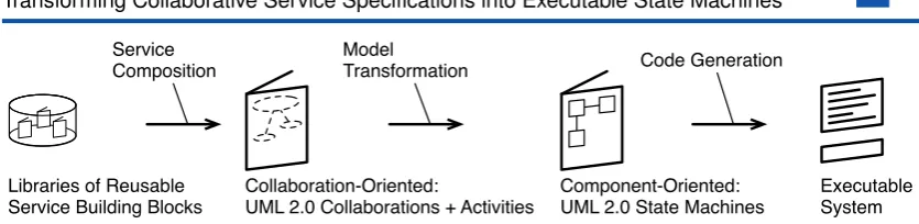
Figure 1: Engineering approach for interactive services
• In the collaboration-oriented perspective, services are modeled by a number of collabora-tions as the main structuring elements. A collaboration specifies the interaccollabora-tions between the components involved in it, as well as the corresponding local behavior of the compo-nents to accomplish the service. Collaborations describe services in a self-contained form and may be composed from other ones. Within an application domain, collaborations contributing to a service are often similar which makes them ideal elements of reuse.
These two perspectives are the shaping forces behind our approach for the rapid engineering of interactive services, outlined in Fig.1. Services are composed from collaborations that identify the interactions as well as the local behavior of a set of components that are necessary to fulfill a certain task. To express the structural aspects of collaborations as well as their composition (e.g., the participants and which roles they play in a service), we use the conforming concept of UML 2.0 collaborations. For the behavioral aspect (e.g., what a collaboration does as well as how collaborations are coupled together), we use UML 2.0 activities.
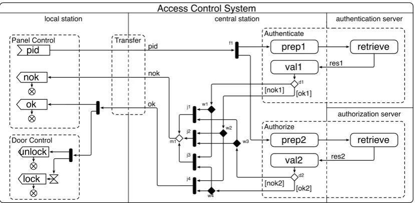
As an example, we consider an access control system (ACS) [6,7]. It controls the opening mechanism of a door and lets pass only authorized people that can prove their identity by pre-senting a security card and a secret number at an input panel. The opening mechanism and input panel are connected to a local station installed close to the door. Once a user draws the card and enters the pin, the resulting data (called pid) is transferred to a central station that authenticates the user and checks authorization right by querying two servers. If both, the authentication and authorization are successful,okis sent back to the local station that opens the door.
local station :Door Control
door
panel
:Panel Control
authorization server :Authenticate
:Authorize
authentication server
central station :Transfer
Figure 2: Collaboration to compose the sub-services of the access control system
Transfer
Door Control
Authenticate
Authorize local station
Access Control System
central station
authorization server authentication server
unlock
lock
nok pid
ok nok
pid prep1
[ok1]
[nok2]
val1
retrieve
prep2
val2
retrieve
[ok2] [nok1]
ok w1
w2 w3
w4
d1
d2 f1
j1
j2
j3
j4 m1
Panel Control
res1
res2
Figure 3: Activity diagram modeling the detailed behavior of the system
development perspectives outlined above. Sect. 6 sketches then a proof of the correctness of the transformation in temporal logic. We close with a discussion of related approaches and some concluding remarks.
2
Collaborations and Activities for Service Composition
Central Station
0
2 Res1/d
nok1 NOK nok2 0 NOK ok2 0 prep1 Req1 Req2 prep2 -* 0 Local Station 0 Res1 0 retrieve 0 Res2 0 retrieve Authentication S. Authorization S. 4 Res1/d
ok1 val1 val2 val2 NOK nok2 0 OK ok2 0 val2 8 Res2/d
nok2 NOK nok1 0 NOK ok1 0 16 Res1/d
ok2 val1 NOK nok1 0 OK ok1 0 val1 Res1 Res2 Res2 PID Req1 Req2
Res2 Res1 Res1
OK unlock 1 set timer lock 0 OK timer * NOK -NOK * PID -PID *
Figure 4: Executable state machines for the system components
door shutter again after a while. As activities have a Petri net like semantics [8], we can use to-kens and places to understand the behavior of the diagram in Fig.3. Once a token representing a pid arrives at the central station, it is prepared (described by the operationsprep1andprep2) and sent to the authentication respective the authorization server. For that, the token is duplicated at the fork nodef1, so that the subsequent behaviors may happen in parallel. Both servers evaluate the pid and send their results back to the central station.
The results may arrive in any order. For example, if the result of the authorization server arrives first, it is evaluated by the central station (operationval2) which branches in decisiond2 depending on the validity of the authorization. If the result was valid, a token is placed inw4. This node is an extension of a decision node (cf. [4]) as tokens can rest in it. It is represented by a filled diamond. The central station waits now for the arrival of the authentication result, which is evaluated inval1, and a token is placed either onw1orw2. When the other result arrives, two waiting decisions hold one token, so that exactly one of the join nodesj1..j4can fire. Obviously, j4fires in the case that both results were ok and causes the central station to send an ok to the local station. In the other three cases (when at least one result isnok) one of the other join nodes j1..j3fires. These cases are combined by merge nodem1and anokis sent to the local station. We assume that the panel control only sends a newpidafter it received anokor anok.
3
State Machines for Service Execution
presented a transition that can be executed from any control state by referring to a state called “*”. After it executes, the state machine returns into its originating state, denoted by “-”.
As these executable state machines are the input for our code generators [9], they must fulfill some constraints to achieve efficient code. In particular, they are event-driven, which means that each transition is only executed as the reaction to either the creation of the state machine itself, the reception of a signal, or the expiration of an internal timer. In consequence, transitions are enabled based purely on their source state and trigger, so that guards may only be declared on branches following choices. Moreover, for each pair of control state and trigger, merely one transition may be declared to prevent fairness conflicts between competing transitions.
These executable state machines have a long tradition in the telecommunication area (see for example [10]) and facilitate the efficient implementation on a range of different platforms and architectures, including J2EE. We defined in [5] their execution semantics in terms of tempo-ral logic and described, how they can be efficiently implemented using a scheduler as virtual machine layer. Of course, the constraints on the executable state machines needed to generate efficient code highly influence the layout of our algorithm which we discuss in the following.
4
Transformation from Activities to State Machines
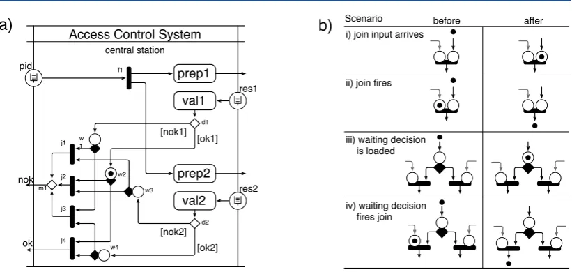
In our approach, an activity partition corresponds to one physical point of execution. We there-fore generate one state machine for each activity partition. This also makes it possible to consider the activity partitions separately and not the entire activity, as discussed later. To separate the partitions from each other, we have to cut those edges which cross partition borders. These edges model the control flows between different system components. As communication between the state machines is done entirely by means of signals, a flow crossing the boundaries of activity partitions must be implemented as a signal transmission. In activities, flows between actions occur instantaneously, i.e., a token leaves an action and enters a subsequent one without resting in the flow. The transmission between state machines, however, is buffered. Introducing signal transmissions in flows between partitions therefore implies virtual places that may hold tokens. We add these places where flows enter a partition, as illustrated in Fig. 5 by the circles with the queue symbols inside. These so-calledqueue places simulate the input queue of the state machines implementing an activity partition. In the model, these input queues are of unlimited capacity1. Thus, the virtual places are unbounded (i.e., can hold any number of tokens).
As described above, the state machines execute a transition as a reaction to the arrival of a signal. This event corresponds to the emission of a token from the virtual queue places. Hence, when we construct a transition, we simulate the emission of one token from a queue place. The token passes along the flows and nodes of the activity diagram until it reaches a control node where it has to wait for further events to happen. These are three kinds of nodes: (1)Join nodes synchronize different flows, that may arrive in any order. An incoming token may have to wait for the other incoming flows to arrive. (2)Waiting decisionssynchronize competing join nodes (see Sect. 2). A token has to rest inside a waiting decision if none of the succeeding joins can fire. (3)Timer nodesmay contain tokens describing that the timers are active.
Fig. 5 (a) illustrates also theinner placesof the central station in which tokens rest to wait for
Access Control System central station
nok pid
prep1
[ok1]
[nok2] val1
prep2 val2
[ok2] [nok1]
ok
w 1
w3
w4
d1
d2 f1
j1
j2
j3
j4 m1
w2
Scenario before i) join input arrives
ii) join fires
after
iv) waiting decision fires join iii) waiting decision is loaded res1
res2
a) b)
Figure 5: (a) Places for the nodes (b) Rules for token transitions
further input events. In contrast to the queue places, these inner places will constitute the control states of the state machine. For instance, the token in the waiting decision w2 of Fig. 5 (a) means that a valid authentication result arrived and that the central node waits for the result of the authorization. (The join nodes do not have own places, as all their incoming flow originate from waiting decisions, which hold the token instead.) For the number of control states to be finite, the number of tokens in an inner place must be bounded. Moreover, to keep the state space small, we allow only one token in each inner place. This is not a limitation since tokens that would fill an inner place are stored in the unlimited queue places as discussed later. The set of control states for one state machine is then the powerset of the inner places.
We can construct a state machine transition by following the passing of the tokens between two stable token markings. The marking of the inner places before passing the tokens define the source state of the transition and the next stable marking refer to the target state. The token taken from a queue place models the input signal consumed by the transition. The activity nodes passed by the token are transformed in the following way: Call operation actions and send signal actions are simply copied into the effect of a transition. Decision nodes with guards are added to the transition and lead to different branches. A flow leaving the current activity partition is translated to a send signal action. Fork nodes duplicate tokens, to that the subsequent flows are executed in parallel. In the transition, this is mapped by executing their actions interleaved. For instance, the transition triggered byPID inCentral Stationin Fig. 4 simply executes first the actionprep1and thenprep2. Initial nodes emit tokens once the activity is started and are treated by the initial transition of a state machine.
is filled with a token (iii), and a new stable state is reached. If one of the joins is ready, the transition continues at its outgoing edge, consuming the token from the decision node(iv).
In addition to the events of signal reception resulting from the split control flows, explicit sig-nal receptions contribute to the set of unbounded queue places. Furthermore, timers are sources of events. When a timeout occurs, a token is emitted on the timer’s outgoing edge. The transi-tion is then constructed in the same way as for signal receptransi-tions. Some events may lead to states describing that an inner place contains more than one token. For example, if the central station is connected to several local stations, a pid could arrive while another pid is under evaluation. In this case it might happen, that, after the central station received a validres1and waits forres2, another validres1is coming, which requires nodew2to hold two tokens. To prevent this, we do not create a transition for flows leading to a marking with several tokens in an inner place, but defer the incoming event, which may proceed after the inner place is emptied.
5
The Transformation Algorithm
To realize the transformation from activities to state machines introduced above, we can proceed in quite different ways. For instance, one could perform a complete reachability analysis over all allowed token allocations in the previously introduced inner and queue places of an activity and create a transition for every step. The disadvantage is that, especially in highly concurrent sys-tems, the number of reachable states is very large, rendering the approach not scalable. Another possibility would be to perform a purely syntactical analysis of an activity. Here, for each edge between places, a set of transitions is generated. Thereby, a separate transition is created for all states in which tokens are contained in the corresponding places. This algorithm is quite efficient since every inner place of the activity is checked only once, but will lead to a large number of transitions leaving unreachable states. To prevent these disadvantages, we follow an intermedi-ate approach. Reflecting that for every activity partition a separintermedi-ate stintermedi-ate machine is creintermedi-ated, we perform a reachability analysis over the states of an activity partition only, which are constituted by its inner places. Thus, the number of reachable states is kept small. Starting from the initial state, for each reached state and every possible input signal a separate transition is created. As we handle each incoming signal in all control states, some of these transitions may be never fired (if their input signal cannot occur in the state). However, an unnecessary transition would simply result in a code fragment that is never executed. While this is not a real problem, nevertheless, we plan to eliminate these transitions using interface descriptions of the other partitions. These interface descriptions may be offered as part of the collaboration building blocks of a library.
In the following, we explain our algorithm in detail. Fig. 6 depicts the main loop (lines7 to 27). As in most reachability analysis algorithms, this loop guarantees that all reachable markings
of an activity partition are analyzed. The markings yet to be checked are listed in the variable reachablewhile visitedcontains all markings which were already analyzed. In the initial part of the algorithm(1..6), a new and empty state machine is created. Thereafter, the first marking to
be checked, the initial transition of the state machine and the set of events to be received by the state machine are computed. As our algorithm creates a state machine transition for each pair of reachable marking and event (see Sect. 4), the loop contains a nested for-loop(10..26)cycling
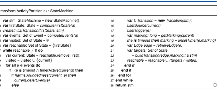
transform(ActivityPartition a) : StateMachine
1 varstm: StateMachine =newStateMachine()
2 varfirstState: State =computeFirstState(a)
3 createInitialTransition(firstState, stm)
4 varevents: Set of Event =computeEvents(a)
5 varvisited: Set of State =/0
6 varreachable: Set of State ={firstState}
7 whilereachable6=/0do
8 varcurrent: State = reachable.removeFirst();
9 visited = visited∪{current}
10 for alle∈eventsdo
11 if¬(e is timeout∧timerActive(current))then
12 ifharmsBoundedness(current, e)then
13 current.deferEvent(e)
14 else
15 vart: Transition =newTransition(stm);
16 t.setSource(current)
17 t.setTrigger(e)
18 varmarking: long = getMarking(current)
19 ifeistimeoutthenmarking = unsetTimer(e,marking)
20 varEdge edge = retrieveEdge(e)
21 vartargets: Set of State
22 = buildTransition(edge,marking,t,a,stm)
23 reachable = reachable∪(targets / visited)
24 end if
25 end if
26 end for
27end while
28returnstm.
Figure 6: Main control
to ignore events triggered by a timer which is not active in the current state. The second if-statement enables us to handle violations of the desired 1-boundedness property correctly. If the traversal of an edge in the checked activity would lead to two or more tokens in any inner place, the algorithm does not create a transition but defers the event in the current state(13). Otherwise,
a new transition is built in the else-statement(15..23).
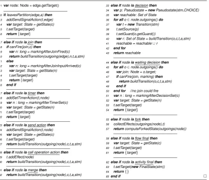
The transitions of a state machine are created by means of the recursive method buildTransi-tion(20), listed in Fig. 7. It considers the traversal of a token from one stable marking to another.
For each edge part of the flow triggered by the event it is called recursively and builds the cor-responding transition along the way. The method returns the set of stable states reached by the transition. It is a set, as a flow may lead to several distinct reachable states after a decision node. The returned states are used by the main loop to determine the reachable markings of the partition yet to be checked. The method contains an order of nested if-statements describing the behavior for each possible node in the analyzed activity edge. It returns if the edge leaves the partition(2),
reaches a join which cannot be fired in the current activity marking(12), starts a timer(17), arrives
at a waiting decision in which none of the corresponding joins can be fired in the current mark-ing(50), or reaches a flow final resp. activity final node (58, 62). In all these cases a new stable
state is reached and the created transition can be completed. When another edge is reached, the transition is not yet complete and its building process has to be continued by a recursive call of buildTransition. These cases are a join which can be executed after being reached by a token on the analyzed edge(10), a send action(27), an operation call(30), a merge(32), a decision(40), a
waiting decision from which a corresponding join can be fired after being reached by a token(48),
and a fork (57). While most steps in creating a transition follow directly the ideas presented in
Sect. 4, we will look now on the decisions and forks which are a little subtle. A decision leads to the addition of a choice pseudo state to the transition behind which more than one continuing transition fragments are added. This is done by the for-loop(36..42)which callsbuildTransition
for each of the choice’s branches. Arriving at a fork(55)means that tokens are emitted at each
buildTransition(Edge edge, long c, Transition t, ActivityPartition a, StateMachine stm) : Set of State
1 varnode: Node = edge.getTarget()
2 ifleavesPartition(edge,a)then 3 addSendSignalAction(t,edge)
4 vartarget: State = getState(c)
5 t.setTarget(target)
6 return{target}
7 else ifnodeisjointhen
8 ifcanFire(join,c)then
9 varn: long = markingAfterJoinFired(c)
10 returnbuildTransition(outgoing(edge),n,t,a,stm)
11 else
12 varn: long = markingAfterJoinInputArrived(c)
13 vartarget: State = getState(n)
14 t.setTarget(target)
15 return{target}
16 end if
17else ifnodeistimerthen
18 addSetTimerAction(t,node)
19 varn : long = markingAfterTimerSet(c)
20 vartarget: State = getState(n)
21 t.setTarget(target)
22 return{target}
23else ifnodeissend actionthen
24 addSendSignalAction(t,node)
25 vartarget: State = getState(c)
26 t.setTarget(target)
27 returnbuildTransition(outgoing(node),c,t,a,stm)
28else ifnodeiscall operation actionthen
29 t.addEffect(node)
30 returnbuildTransition(outgoing(node),c,t,a,stm)
31else ifnodeismergethen
32 returnbuildTransition(outgoing(node),c,t,a,stm)
33else ifnodeisdecisionthen
34 varp: Pseudostate =newPseudostate(stm,CHOICE)
35 varreachable: Set of State
36 for allo∈node.outgoings()do
37 vart =newTransition(stm)
38 t.setSource(p)
39 t.setGuard(o.getGuard())
40 varr: Set of State = buildTransition(o,c,t,a,stm)
41 reachable = reachable∪r
42 end for
43 returnreachable
44else ifnodeiswaiting decisionthen
45 for allo∈node.outgoings()do
46 varjoin: Node = o.target;
47 ifcanFire(join, marking)then
48 returnbuildTransition(o,c,t,a,stm)
49 end if
50 end for //no join could fire
51 varn : long = markingAfterDecisionSet(c)
52 vartarget: State = getState(n)
53 t.setTarget(target)
54 return{target}
55else ifnodeisforkthen
56 collectEffects(outgoings(node),t)
57 returncomputeForkedState(outgoings(node))
58else ifnodeisflow finalthen
59 vartarget: State = getState(c)
60 t.setTarget(target)
61 return{target}
62else ifnodeisactivity finalthen
63 t.setTarget(newFinalState(stm))
64 return{}
65end if
Figure 7: Method to build a transition
6
Correctness of the Transformation
To verify that the algorithm carries out transformations in a correctness-preserving manner, we use the linear-time temporal logic cTLA [12] as a formalismwhich is based on Leslie Lam-port’s TLA [13]. cTLA enables the description of resources and constraints in a process-like notion and provides a coupling structure based on conjoining actions (i.e., predicates on pairs of states describing sets of transitions). Refinement verifications are carried out as temporal logic implication proofs (cf. [13]). As the semantics of activities is based on Petri-nets [8], UML 2.0 activities can easily be expressed by cTLA processes as pointed out in [14]. An activity, ba-sically, is a cTLA system description consisting of processes each describing a single activity partition. The variables of a process model its inner places while each queue place of a partition is described by a separate input queue.
reflects that the transition depends only on the current state and the first signal in the input queue. Moreover, each component contains an extra queue to handle deferred events. The re-finement of specifications modeling activities to cTLA/e-based descriptions is carried out by a sequence of correctness-preserving refinement steps accompanied by cTLA/TLA implication proofs (cf. [13]). For the sake of brevity, we do not give a thorough introduction to cTLA here and sketch the proof steps only briefly.
To verify formally that a state machineSderived from an activity partitionAkeeps all the func-tional properties state byA, we must perform by temporal logic deductions that the implication S⇒Aholds. According to Abadi and Lamport [15], this can be achieved by finding a so-called refinement mapping from the states ofSto those ofA. A refinement mapping takes into account that cTLA enables the modeling of state transition systems. A system formula consists of an initial condition describing the set of initial states, cTLA actions which are predicates on a pair of a current state and a next state and model a set of state transitions each, and liveness properties expressed by fairness assumptions on actions which enforce that actions are eventually executed when they are consistently enabled. A refinement mapping has to keep the following properties:
• An initial state ofSis mapped to an initial state ofA.
• Each cTLA action ofSis either mapped to an action ofAor to a so-called stuttering step in which the mapped current and next states ofAare identical.
• Each fairness assumption of A is provided by the fairness assumptions of S (i.e., if an actionψ ofAis consistently enabled, the fairness actions ofSenforce a state sequence in which eventually an action is carried out which is mapped toψ).
In Sec. 4 we stated that the state space of an activity partitionAis partly defined by its inner places which are situated before joins, at decision nodes, at initial nodes, and at timers. Moreover, it contains queue places which are situated at points where an incoming flow passes the partition border and on receive actions. The state space of a state machine is defined in [5] and consists of the literal states of the state machine, an input queue, a defer queue, output queues for all connected state machines, and flags for each timer. Furthermore, activities may contain auxiliary variables which our algorithm directly maps to auxiliary variables of the corresponding state machines. To outline the correctness of the algorithm, we will, in the following, list a mapping of the state space fromSto that ofAand sketch thereafter that it keeps the refinement mapping properties:
• To find a mapping fromSto the queue places ofA, we have also to consider the linked state machines as the queue places mainly describe the interaction between different system elements. At an activity partition, we have a separate queue place for every signal typest while in the corresponding state machine, we have central queues for all signals. Moreover, in the activity we do not distinguish if a signal is still at the side of the outgoing partition, already in the incoming partition, or deferred. Reflecting these properties, we map all signalss of typest, which are either in the output queue of a neighboring state machine Sn, in the input queue ofS, or in its defer queue, to the queue placeqpst forstinA:
∀st:qpst={s|s.type=st∧s∈inputQS∪de f erQS∪ [
Sn∈NeighborsS
• A mapping ofSto the inner places ofAlocated at joins, decision nodes, and initial nodes has to consider that we use 1-boundedness in the inner placesip and that the algorithm creates the states ofSas a string of flags f lipeach being set to 0 if the corresponding inner placeipis empty and to 1 ifipcontains a tokento:
∀ip:ip=IFf lip=1 THEN{to}ELSE{}
• To find a mapping from S to the inner places of A describing a timer is a little more complex. Indeed, the algorithm adds also a flag ft for each timertinAto the state repre-sentation inS. Nevertheless, to find a decent mapping one has to consider the handling of timers in state machines. When a timer expires, it creates a signal which is attached to the local input queue. Thus, we must map both the states ofSin which the flag f lt of timert is enabled and in which a signalst caused bytis in the input or defer queue to a setting in Awhere a tokentois on the inner placeipt oft. That is expressed by the mapping listed below:
∀ipt :ipt=IFf lt=1∨st ∈inputQS∪de f erQSTHEN{to}ELSE{}
• The mapping from the auxiliary variables fromSto those ofAis the identity function.
In the first step of the proof that the function listed above fulfills the refinement mapping properties, we have to verify that the initial state ofSis mapped to that ofA. Initially, the queue places inAare empty while the input, output, and defer queues ofSdo not contain elements as well. Thus, the mapping of the queue places fulfills the property trivially. The inner places of Aare empty except those located at an initial node. As discussed in Sec. 5, the algorithm maps the token placement of an initial state ofSin which just the flags representing the inner places of the initial nodes are set to 1. Since the auxiliary variables ofSandAcontain the same initial settings, therefore, the initial state ofSis mapped to the initial state ofA.
Next, we prove that every cTLA action in the model of the state machineSis mapped either to a cTLA action of the activity partitionAor to a stuttering step. As introduced in [5], the model ofS contains different kinds of actions. One type describes the transitions of S and for each transitiontrf, a cTLA actionφtrf is defined. The algorithm creates trf only if a flow f exists
modifying the token setting ofA. In the following, we state a number of properties preserved by the algorithm in the creation of the corresponding transitiontrf which are used for the refinement proof:
1. A transitiontrf is only created if in its source state all flags f liprepresenting those inner placesipof f are set to 1 which have to contain tokens in order to execute f.
2. The algorithm creates trf only for a flow f if the execution of f does not violate the inboundedness property of the inner places inA.
3. If the queue place in f, from which a token is removed, has the typest,trf is only triggered ifstis at the front of the input queue.
4. By executing a transitiontrf which does not leave an initial state, the signal at the front of the input queue is consumed.
6. The target states oftrf are generated by starting with the source state and resetting the flags representing inner places, from which tokens were removed, to 0 while those with a new token are set to 12.
7. If in f a token is heading to the partition border with a partitionAnor to a send action with destinationAn,trf puts a send signal into the output queue devoted to the state machineSn realizingAn.
8. A call operation action passed in f is reflected by adding its code totrf. Here, we demand that an auxiliary variable may be modified only once in f and, in consequence, intrf.
Assuming thatφtrf is the cTLA action modelingtrf andψf those of the flow f, these properties
are sufficient to prove the implication φtrf ⇒ψf. By the first three properties, we can assure
that the enabling condition ofφtrf implies that oψf since according to the mapping all necessary
tokens are set (1), the 1-boundedness after carrying out f is preserved (2), and the queue place from which f leaves contains an element (3).
The other properties are used to verify that the effects of φtrf are correctly mapped to those
ofψf. The elimination of a signal of typestfrom the input queue is mapped to the removal of a token from the queue placest (4). In addition, iftrf consumes a signalst created by a timer from the input queue,st is mapped to a flow f removing a token from the corresponding timer node (5). We can further verify thattris a correct realization of the token flow between the inner places in f (6). The delivery of a signals to an adjacent state machineSn does not spoil the corresponding mapping ofSnto a neighboring activity partitionAnassis added to an incoming queue place ofAnifSputs it to its output queue devoted toSn(7). Finally, it is guaranteed that the auxiliary variables are correctly mapped (8). It is not difficult to verify that these properties imply that the mapping listed above mapsφtrf toψf which is omitted, however, for brevity.
Other cTLA actions inSspecify the execution of timers and the addition of timer signals to the input queue, model the deferral of a signal by transferring it from the input to the defer queue, and describe the transfer of signals from the neighbor’s output queue to the own input queue. It can be easily shown that these actions lead to stuttering steps inA.
In the third step, we have to verify that the fairness assumptions of the actionsψf describing the flows inAare kept. The algorithm guarantees that for every token placement in the inner nodes ofAenabling a flow f, a transitiontrf is generated implementing f. Thus, with respect to the first two properties listed above, an actiontrf is enabled whenever f can fire. The only impeding condition is the third property sincetrf may only be executed if the signalsconsumed by it is at the first place of the input queue. According to the mapping, however, the cTLA action
ψf specifying fcan be enabled ifsis either in the output queue of the neighboring state machine Sn or in any place on the input or defer queues ofS. Thus, we must verify that sis eventually being moved to the front of the input queue where it will remain consistently until an actionφtrf
is executed. Ifsis still in the output buffer ofSn, it will be moved to the end of the input buffer of Sby the fair3action modeling the transmission fromSntoS. Since signals beforesin the input resp. defer queue are either continuously being deferred4or eventually being consumed. Thus, 2 If a token is both removed from and added to an inner place in the same flow, its flag remains set to 1.
3 In [12] we established that liveness can only be guaranteed in a distributed system if transmitted messages
are eventually being delivered. This property is expressed by the fairness assumption on the action specifying the transmission.
swill be eventually at the front of the input queue. If f is not enabled,smay be deferred itself but is brought back to the front of the input queue by other transitions. As there is only a finite number of transitionstrf modeling f, in consequence, one of those will be consistently being enabled if f can be triggered as well. Due to the fairness assumption of the corresponding cTLA actionφtrf it will be eventually fired which, because of the mapping, causes also the triggering
of f.
Thus, we could verify that the mapping listed above is a refine mapping. According to [15], we could thereby prove that the state machineStogether with its neighboring state machinesSn produced by the algorithm is a correct implementation of the activity partitionA. Since this prove can be carried out for all partitions of the activity, we established that the algorithm transforms activities to state machines in a correct way.
7
Related Work
To our best knowledge, the algorithm presented here is the first one that directly transforms UML 2.0 activity diagrams into the executable state machines described above. Our work is related to that of Eshuis on model checking of activity diagrams [11], in which activity diagrams are transformed into the input language of NuSMV, a symbolic model verifier [16]. We could not adapt this algorithm for our work, since, as discussed in Sect. 5, syntactical algorithms cause in our field of application a high number of considered unreachable states. To execute activity graphs, Eshuis and Wieringa [17] describe an algorithm for an event router to coordinate the behavior of components. Aiming at workflow systems, their execution differs from ours as it assumes a centralized architecture and the activity is considered as a whole, rather than splitting up the activity into its partitions and creating distributed state machines as we do.
8
Concluding Remarks
We described an algorithm that transforms UML 2.0 activities into a UML 2.0 state machines, from which we can easily generate efficiently executable code. The algorithm is implemented in Java and integrated into our Eclipse-based tool suite, so that we now have a complete automated development process from collaborative specifications based on activities to implementations on various platforms. As input and output we use models stored in the Java UML 2.0 repository from the Eclipse UML2 project. The algorithm does not construct an intermediate graph, but only UML model elements that are part of the desired output state machines, so that it is efficient with respect to the memory needed. The time for the transformation of the presented example is negligible; the state machines appear practically instantly. Moreover, we expect the algorithm to scale well also for more complex systems, as the increased complexity of a system leads more to a higher number of partitions than to more complex ones causing only a linear increase.
This work describes a step of a more comprehensive engineering approach for the creation of interactive services by correctness-preserving design steps. Initially, a service specification is composed from various abstract collaborations that, to a large extent, can be obtained from domain-specific libraries. Such abstract collaborations are often quite simple and can also be understood by customers, who are not experts in software technology but want to focus on their actual business. In succeeding steps, such abstract specifications are incrementally refined until the specification has a degree of detail that enables direct translation to software. Due to the algorithm, we are now able to perform these refining design steps entirely in the collaboration-oriented perspective. As pointed out in [4], for this purpose we can use the activities with their convenient properties as reusable building blocks.
Bibliography
[1] Floch, J., Bræk, R.: Towards Dynamic Composition of Hybrid Communication Services. 6th Int. Conf. on Intelligence in Networks (SMARTNET), Deventer, Kluwer, (2000)
[2] R¨oßler, F., Geppert, B., Gotzhein, R.: Collaboration-Based Design of SDL Systems. 10th Int. SDL Forum on Meeting UML, Springer-Verlag (2001) 72–89
[3] Sanders, R.T., Castej´on, H.N., Kraemer, F.A., Bræk, R.: Using UML 2.0 Collaborations for Compositional Service Specification. In: ACM / IEEE 8th Int. Conf. on Model Driven Engineering Languages and Systems. (2005)
[4] Kraemer, F.A., Herrmann, P.: Service Specification by Composition of Collaborations — An Example. 2nd Int. Workshop on Service Composition (Sercomp), Hong Kong (2006)
[5] Kraemer, F.A., Herrmann, P., Bræk, R.: Aligning UML 2.0 State Machines and Tempo-ral Logic for the Efficient Execution of Services. Int. Conf. on Distributed Objects and Applications (DOA), 2006, Montpellier, LNCS 4276, Springer (2006) 1613–1632
[7] Broy, M., Stølen, K.: Specification and Development of Interactive Systems: Focus on Streams, Interfaces, and Refinement. Springer (2001)
[8] Object Management Group: Unified Modeling Language: Superstructure (2006)
[9] Kraemer, F.A.: Rapid Service Development for Service Frame. Master’s thesis, University of Stuttgart (2003)
[10] Bræk, R.: Unified System Modelling and Implementation. Int. Switching Symposium, Paris, France (1979) 1180–1187
[11] Eshuis, R.: Symbolic Model Checking of UML Activity Diagrams. ACM Transactions on Software Engineering and Methodology15(1) (2006) 1–38
[12] Herrmann, P., Krumm, H.: A Framework for Modeling Transfer Protocols. Computer Networks34(2) (2000) 317–337
[13] Lamport, L.: Specifying Systems. Addison-Wesley (2002)
[14] Graw, G., Herrmann, P.: Transformation and Verification of Executable UML Models. Electronic Notes on Theoretical Computer Science, Elsevier Science101(2004) 3–24
[15] Abadi, M., Lamport L.: The Existence of Refinement Mappings. Theoretical Computer Science82(2) (1991) 253–284
[16] Cimatti, A., Clarke, E.M., Giunchiglia, E., Giunchiglia, F., Pistore, M., Roveri, M., Sebas-tiani, R., Tacchella, A.: NuSMV 2: An Opensource Tool for Symbolic Model Checking. 14th Int. Conf. on Computer Aided Verification (CAV), LNCS 2404, Springer (2002)
[17] Eshuis, R., Wieringa, R.: An Execution Algorithm for UML Activity Graphs. 4th Int. Conf. on The Unified Modeling Language, Modeling Languages, Concepts, and Tools (UML), London, Springer (2001) 47–61
[18] Mansurov, N., Zhukov, D.: Automatic Synthesis of SDL Models in Use Case Methodology. In Dssouli, R., von Bochmann, G., Lahav, Y., eds.: SDL Forum, Elsevier (1999) 225–240
[19] Whittle, J., Schumann, J.: Generating Statechart Designs from Scenarios. 22nd Int. Conf. on Software Engineering (ICSE), New York, ACM Press (2000) 314–323
[20] Kr¨uger, I., Grosu, R., Scholz, P., Broy, M.: From MSCs to Statecharts (1999)
[21] Uchitel, S., Kramer, J., Magee, J.: Synthesis of Behavioral Models from Scenarios. IEEE Trans. Softw. Eng.29(2) (2003) 99–115
[22] Buhr, R.J.A., Casselman, R.S.: Use Case Maps for Object-Oriented Systems. (1996)
[23] He, Y., Amyot, D., Williams, A.W.: Synthesizing SDL from Use Case Maps: An Experi-ment. 11th SDL Forum, Stuttgart. LNCS 2708, Springer (2003) 117–136