Volume 2014, Article ID ama0135, 12 pages ISSN 2307-7743
http://scienceasia.asia
MODELING INTERACTIONS OF NILE PERCH, NILE TILAPIA AND SMALL PELAGIC SILVER FISH WITH CONSTANT
HARVESTING EFFORTS IN LAKE VICTORIA
JAMES PHILBERT MPELE, OLUWOLE DANIEL MAKINDE, YAW NKANSAH-GYEKYE
Abstract. In this paper, we examined the effects of interactions in a predator-prey manner and harvesting at constant fishing efforts of Nile perch (Lates niloticus), Nile tilapia (Oreochromis niloticus) and Small pelagic silver ( Ras-trineobola argentea) fish species of the lake Victoria fishery, through mathe-matical modeling using Lotka-Volterra equation, whereby all three fish species are subjected to harvesting. The model is characterized by the system of first order non-linear ordinary differential equations.
All eight equilibrium points of the model were identified, the local stability of the co-existence equilibrium point was discussed using Routh-Hurwitz criteria and its global stability was analyzed using suitable Lyapunov function. Fur-ther, analytic solutions of the model coincided with the computed numerical solutions using fourth order Runge-Kutta method. The study revealed that as the model parameters became small the equilibrium stock level biomasses of fish species increased.
1. INTRODUCTION
Lake Victoria is the second largest fresh-water lake in the world and the largest in Africa. The lake is shared by Kenya (6%), Uganda (43%) and Tanzania (51%). According to [7], lake Victoria fishery is currently dominated by three fish species which are Nile perch, Nile tilapia and small pelagic silver fish. The lake is an im-portant source of food, employment and earnings for the riparian states through fishery for millions of people.
The study aims at investigating the effects of harvesting at constant fishing ef-forts and interactions in a predator-prey manner to the equilibrium stock level biomasses of Nile perch, Nile tilapia and small pelagic silver fish species in lake Victoria. The Nile perch are predator to Nile tilapia and vice versa (depending on their sizes, that is, adult Nile perch eats the young Nile tilapia and adult Nile tilapia eats the young Nile perch) while small pelagic silver fishes are prey to both Nile perch and Nile tilapia.
Quantitative and qualitative understanding of the interactions of these fish species is crucial for the management of fisheries in lake Victoria. Harvesting has generally a strong impact on the population dynamics of harvested species. The severity of this impact depends on the nature of the applied harvesting strategy which, in turn,
2010Mathematics Subject Classification. 92-08, 65P99, 92B05, 37N25.
Key words and phrases. Lake Victoria, Nile perch, Nile tilapia, small pelagic silver fish, co-existence, Lotka-Volterra, Lyapunov function, Runge-Kutta.
c
may range from the rapid depletion to the complete preservation of a population[10].
The problem of interspecies interactions was considered by [4] for two species obeying the law of logistic growth. [2] considered harvesting of a single species in an ecologically competing two fish population model.[1] and [11] studied the dynamics of two-species fishery by combining harvesting. [3] studied constant rate of harvesting in a predator-prey system to allow simultaneous harvesting of both species. They showed how to approximate the region of asymptotic stability in biological terms, in the initial states which lead to coexistence of the two species and their global dynamics by efficient computer simulation. [9] studied the effect of Nile perch predation to Nile tilapia and harvesting on fisheries dynamics in Lake Victoria, the study ignored the third species, the small pelagic silver fish, a prey to the first two species which has a significant contribution to the dynamics of species.To the authors’ knowledge,the nature of this study has not yet been done.
2. MATHEMATICAL MODEL
2.1. Assumptions of the model. The model rely on the following assumptions:
• The fish species can grow independently in a lake and their population sizes are bounded
• Adult Nile perch are predator to both young Nile tilapia and Small pelagic silver fish
• Adult Nile tilapia are predator to both young Nile perch and Small pelagic silver fish
• Small pelagic silver fishes are prey to both Nile tilapia and Nile perch
• All three fish species have ecological interactions in a lake
• All three fish species are harvested at a rate proportional to the size of their population
• Fishing effort for all fish species is kept constant
2.2. Definitions of variables and parameters of the model. The fol-lowing are the definitions of variables and parameters used in developing the model:
r1: intrinsic growth rate of Nile perch
r2: intrinsic growth rate of Nile tilapia
r3: intrinsic growth rate of small pelagic silver fish
x: stock biomass of Nile perch y: stock biomass of Nile tilapia
z: stock biomass of small pelagic silver fish α: predation rate of Nile tilapia to Nile perch β: predation rate of Nile perch to Nile tilapia
γ: predation rate of Nile perch to small pelagic silver fish ψ: predation rate of Nile tilapia to small pelagic silver fish E1: fishing effort for Nile perch
E2: fishing effort for Nile tilapia
E3: fishing effort for small pelagic silver fish
q1: catchability coefficient of the Nile perch
q3: catchability coefficient of small pelagic silver fish
K1: carrying capacity of Nile perch
K2: carrying capacity of Nile tilapia
K3: carrying capacity of small pelagic silver fish
2.3. Model equations. The model equations for the three fish species is the set of non-linear ordinary differential equations:
(2. 1) dx
dt =x(c1−a1x−ρy+γz)
(2. 2) dy
dt =y(c2+ρx−a2y+ψz)
(2. 3) dz
dt =z(c3−γx−ψy−a3z)
where ai = ri Ki
>0 fori= 1,2,3 , cj =rj−qjEj >0 for j = 1,2,3 and
(α−β) =ρ >0
3. EXISTENCE OF EQUILIBRIUM POINTS
The system under investigation has eight possible equilibrium points
ob-tained by setting dx dt =
dy dt =
dz
dt = 0.These includes:
(i)E1(x∗, y∗, z∗) = (0,0,0) (absence of all fish species)
(ii)E2(x∗, y∗, z∗) =
0,0,c3 a3
(absence of Nile perch and Nile tilapia)
(iii)E3(x∗, y∗, z∗) = c
1
a1
,0,0
(absence of Nile tilapia and small pelagic
silver fish)
(iv)E4(x∗, y∗, z∗) =
0, c2 a2
,0
(absence of Nile perch and small pelagic
silver fish)
(v)E5(x∗, y∗, z∗) = −c
2ρ+a2c1
ρ2+a 1a2
,a1c2+c1ρ ρ2+a
1a2
,0
(absence of small pelagic
silver fish). The equilibrium pointE5 is positive ifa2c1> c2ρhold.
(vi)E6(x∗, y∗, z∗) =
a3c1+c3γ
γ2+a 1a3
,0,−−a1c3+c1γ
γ2+a 1a3
(absence of
Nileti-lapia).The equilibrium pointE6is positive ifa1c3> c1γ hold.
(vii)E7(x∗, y∗, z∗) =
0,ψc3+a3c2 ψ2+a
2a3
,a2c3−c2ψ ψ2+a
2a3
(absence of Nileperch).
The equilibrium pointE7 is positive ifa2c3> c2ψhold.
(viii)E8 x∗ y∗ z∗ =
−ρψc3−a3ρc2−γψc2+γc3a2+c1ψ2+a2a3c1
a3ρ2+a1ψ2+a1a2a3+γ2a2
a1a3c2+a3c1ρ+ργc3+c2γ2−γψc1+ψc3a1
a3ρ2+a1ψ2+a1a2a3+γ2a2
−(−γρc2+γc1a2+ψc2a1+ψρc1−c3ρ2−c3a1a2)
a3ρ2+a1ψ2+a1a2a3+γ2a2
(the co-existence of all three fish species).The equiliribrium point E8 is
γc3a2+c1ψ2+a2a3c1> ρψc3+a3ρc2+γψc2,
a1a3c2+a3c1ρ+ργc3+c2γ2+ψc3a1> γψc1 and
γρc2+c3ρ2+c3a1a2> γc1a2+ψc2a1+ψρc1
3.1. Local stability analysis. The local stability of the interior equi-librium point (co-existence point E8) was investigated using the
Routh-Hurwitz’s criteria. That is, an equilibrium point is locally asymptotically stable if the characteristic equation of the Jacobian matrix evaluated at that point has all the coefficients being positive and that all of its roots have negative real parts[8].
J(E8) =
c1−2a1x∗−ρy∗+γz∗ −ρx∗ γx∗
ρy∗ c2+ρx∗−2a2y∗+ψz∗ ψy∗
−γz∗ −ψz∗ c3−γx∗−ψy∗−2a3z∗
The characteristic equation ofJ(E8) is
(3. 4) λ3−(b1+b2+b3)λ2+ (b1b2+b2b3+b1b3)λ−(b1b2b3+b4) = 0
where
b1=c1−2a1x∗−ρy∗+γz∗=−a1x∗<0 since, x∗>0 and
c1−a1x∗−ρy∗+γz∗= 0
b2=c2+ρx∗−2a2y∗+ψz∗=−a2y∗<0 since, y∗>0 and
c2+ρx∗−a2y∗+ψz∗= 0
b3=c3−γx∗−ψy∗−2a3z∗=−a3z∗<0 since,z∗>0 and
c3−γx∗−ψy∗−a3z∗= 0
b4=ψ2y∗z∗>0
Hence
(b1+b2+b3)<0 ⇒ −(b1+b2+b3)>0
Similary, (b1b2+b2b3+b1b3)>0
And
b1b2b3+b4 = −a1a2a3x∗y∗z∗+ψ2y∗z∗
= y∗z∗(ψ2−a1a2a3x∗)
Certainly,a1a2a3x∗> ψ2
Hence,b1b2b3+b4=y∗z∗ ψ2−a1a2a3x∗<0⇒ −(b1b2b3+b4)>0
The conditions for Routh-Hurwitz’s criteria are satisfied, that is,
−(b1+b2+b3)(b1b2+b2b3+b1b3)>−(b1b2b3+b4)
Therefore, the co-existence equilibrium point E8 is locally
asymptoti-cally stable.
3.2. Global stability analysis. Global stability of the system was anal-ysed by considering suitable Lyapunov function [5].
Consider the following Lyapunov function candidate,
(3. 5) V(x, y, z) =l1[x−x∗−x∗ln(
x
x∗)]+l2[y−y
∗−y∗ln(y
y∗)]+l3[z−z
∗−z∗ln( z z∗)]
As per, [6], it is evident that the choosen Lyapunov function candi-dateV(x, y, z) of ( 3. 5 ) satisfy the conditions thatV(x∗, y∗, z∗) = 0 and V(x, y, z)>0 for all (x, y, z)6= (x∗, y∗, z∗). Moreover, V(x, y, z) is radially unbounded.
We are required to verify that dV
dt ≤ 0 for the suitable choice of l1 > 0,l2>0 andl3>0.
dV
dt = l1(1− x∗
x) dx
dt +l2(1− y∗
y ) dy
dt +l3(1− z∗
z ) dz dt
= l1(
x−x∗
x )
dx dt +l2(
y−y∗
y )
dy dt +l3(
z−z∗
z )
dz dt
Let
(3. 6) dV
dt =F+G+H where,
F =l1(x−x∗)(c1−a1x−ρy+γz)
G=l2(y−y∗)(c2+ρx−a2y+ψz)
H =l3(z−z∗)(c3−γx−ψy−a3z)
Considering,
F = l1(x−x∗)(c1−a1x−ρy+γz)
= l1[x(c1−a1x−ρy+γz)−x∗(c1−a1x−ρy+γz)]
= l1[c1x−a1x2−ρxy+γxz−c1x∗+a1xx∗+ρyx∗−γzx∗]
Since,c1−a1x∗−ρy∗+γz∗= 0,⇒c1=a1x∗+ρy∗−γz∗
Then
F = l1[x(a1x∗+ρy∗−γz∗)−a1x2−ρxy+γxz − x∗(a1x∗+ρy∗−γz∗) +a1xx∗+ρyx∗−γzx∗]
= l1[−a1(x2−2xx∗+x∗ 2
)−ρ[y(x−x∗)−y∗(x−x∗)]
+ γ[−z∗(x−x∗) +z(x−x∗)]]
Further algebraic simplification gives,
(3. 7) F=l1(x−x∗) [−a1(x−x∗)−ρ(y−y∗) +γ(z−z∗)]
Considering,
G = l2(y−y∗)(c2+ρx−a2y+ψz)
= l2[y(c2+ρx−a2y+ψz)−y∗(c2+ρx−a2y+ψz)]
= l2 c2y+ρxy−a2y2+ψyz−c2y∗−ρxy∗+a2yy∗−ψy∗z
Since,c2+ρx∗−a2y∗+ψz∗= 0, ⇒c2=−ρx∗+a2y∗−ψz∗
Then
G = l2[y(−ρx∗+a2y∗−ψz∗) +ρxy−a2y2+ψyz
− y∗(−ρx∗+a2y∗−ψz∗)−ρxy∗+a2yy∗−ψy∗z]
= l2[−a2(y−y∗)2+ρ[−x∗(y−y∗) +x(y−y∗)]
Further algebraic simplification gives,
(3. 8) G=l2(y−y∗) [ρ(x−x∗)−a2(y−y∗) +ψ(z−z∗)]
Considering,
H = l3(z−z∗)(c3−γx−ψy−a3z)
= l3[z(c3−γx−ψy−a3z)−z∗(c3−γx−ψy−a3z)]
= l3
zc3−γxz−ψyz−a3z2−c3z∗+γxz∗+ψyz∗+a3zz∗
Since,c3−γx∗−ψy∗−a3z∗= 0, ⇒c3=γx∗+ψy∗+a3z∗
Then
H = l3[z(γx∗+ψy∗+a3z∗)−γxz−ψyz−a3z2
− z∗(γx∗+ψy∗+a3z∗) +γxz∗+ψyz∗+a3zz∗]
= l3[−a3(z−z∗)2−γ(x−x∗)(z−z∗)
− ψ(y−y∗)(z−z∗)]
Further algebraic simplification gives
(3. 9) H =l3(z−z∗) [−γ(x−x∗)−ψ(y−y∗)−a3(z−z∗)]
Substituting ( 3. 7 ),( 3. 8 ) and ( 3. 9 ) into ( 3. 6 ) gives,
(3. 10) dV
dt =l1X(−a1X−ρY+γZ)+l2Y(ρX−a2Y+ψZ)+l3Z(−γX−ψY−a3Z)
where,X = (x−x∗),Y = (y−y∗) andZ = (z−z∗)
Further simplification of ( 3. 10 ) gives the following: (3. 11)
dV dt =−
l1a1X2+l2a2Y2+l3a3Z2+[ρ(l2−l1)XY +γ(l1−l3)XZ+ψ(l2−l3)Y Z]
If (X, Y, Z) = (0,0,0), that is, when [x=x∗,y =y∗ andz =z∗] then dV
dt = 0.
And, ifl1=l2=l3, then dVdt <0, for all (x∗, y∗, z∗)6= (x, y, z) inR3. Therefore, the co-existence equilibrium point E8 is globally
asymptoti-cally stable.
4. NUMERICAL EXAMPLES
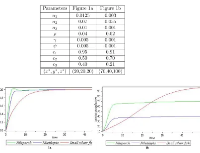
Table 1. Parameters for figure 1a and figure 1b of co-existence
equilibrium pointE8
Parameters Figure 1a Figure 1b
a1 0.0125 0.003
a2 0.07 0.055
a3 0.01 0.001
ρ 0.04 0.02
γ 0.005 0.001
ψ 0.005 0.001
c1 0.95 0.91
c2 0.50 0.70
c3 0.40 0.21
(x∗, y∗, z∗) (20,20,20) (70,40,100)
Figure 1. Graphical representations of the parameters in Table 1
4.1. Examples 1&2with x(0) = 10,y(0) = 10 and z(0) = 10for both cases.
Table 2. Parameters for figure 2a and figure 2b of co-existence equilibrium pointE8
Parameters Figure 2a Figure 2b
a1 0.0015 0.002
a2 0.005 0.0035
a3 0.001 0.0005
ρ 0.002 0.0002
γ 0.001 0.0005
ψ 0.001 0.0005
c1 0.75 0.22
c2 0.60 0.22
c3 0.90 0.225
Figure 2. Graphical representations of the parameters in Table 2
4.2. Examples 3&4with x(0) = 10,y(0) = 10 and z(0) = 10for both cases.
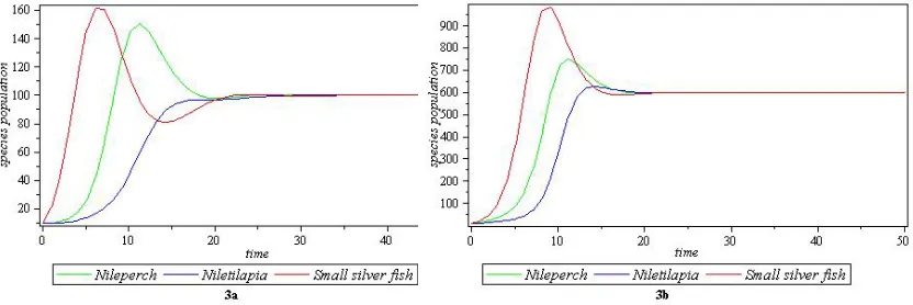
Table 3. Parameters for figure 3a and figure 3b of co-existence
equilibrium pointE8
Parameters Figure 3a Figure 3b
a1 0.0015 0.0008
a2 0.003 0.001
a3 0.004 0.0005
ρ 0.002 0.0003
γ 0.0035 0.0004
ψ 0.001 0.0004
c1 0 0.42
c2 0 0.18
c3 0.85 0.78
(x∗, y∗, z∗) (100,100,100) (600,600,600)
4.3. Examples 5&6with x(0) = 10,y(0) = 10 and z(0) = 10for both cases.
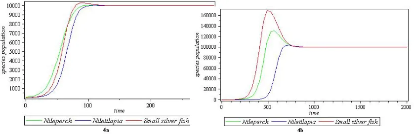
Table 4. Parameters for figure 4a and figure 4b of co-existence
equilibrium pointE8
Parameters Figure 4a Figure 4b
a1 0.000013 0.00000024
a2 0.000015 0.00000022
a3 0.000004 0.00000008
ρ 0.000001 0.00000004
γ 0.000004 0.00000008
ψ 0.000004 0.00000008
c1 0.10 0.020
c2 0.10 0.010
c3 0.12 0.024
(x∗, y∗, z∗) (10000,10000,10000) (100000,100000,100000)
Figure 4. Graphical representations of the parameters in Table 4
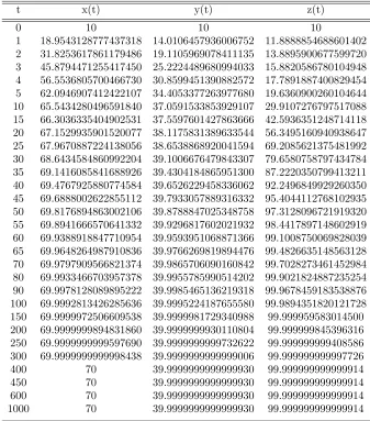
Table 5. Runge-Kutta numerical results for the parameters of figure 1b
t x(t) y(t) z(t)
0 10 10 10
1 18.9543128777437318 14.0106457936006752 11.8888854688601402 2 31.8253617861179486 19.1105969078411135 13.8895900677599720 3 45.8794471255417450 25.2224489680994033 15.8820586780104948 4 56.5536805700466730 30.8599451390882572 17.7891887400829454 5 62.0946907412422107 34.4053377263977680 19.6360900260104644 10 65.5434280496591840 37.0591533853929107 29.9107276797517088 15 66.3036335404902531 37.5597601427863666 42.5936351248714118 20 67.1529935901520077 38.1175831389633544 56.3495160940938647 25 67.9670887224138056 38.6538868920041594 69.2085621375481992 30 68.6434584860992204 39.1006676479843307 79.6580758797434784 35 69.1416085841688926 39.4304184865951300 87.2220350799413211 40 69.4767925880774584 39.6526229458336062 92.2496849929260350 45 69.6888002622855112 39.7933057889316332 95.4044112768102935 50 69.8176894863002106 39.8788847025348758 97.3128096721919320 55 69.8941666570641332 39.9296817602021932 98.4417897148602919 60 69.9388918847710954 39.9593951068871366 99.1008750069828039 65 69.9648264987910836 39.9766269819894476 99.4826635148563128 70 69.9797909566821374 39.9865706090160842 99.7028273461452984 80 69.9933466703957378 39.9955785990514202 99.9021824887235254 90 69.9978128089895222 39.9985465136219318 99.9678459183538876 100 69.9992813426285636 39.9995224187655580 99.9894351820121728 150 69.9999972506609538 39.9999981729340988 99.999959583014500 200 69.9999999894831860 39.9999999930110804 99.999999845396316 250 69.9999999999597690 39.9999999999732622 99.999999999408586 300 69.9999999999998438 39.9999999999999006 99.999999999997726
400 70 39.9999999999999930 99.999999999999914
450 70 39.9999999999999930 99.999999999999914
600 70 39.9999999999999930 99.999999999999914
Table 6. Runge-Kutta numerical results for the parameters of figure 3a
t x(t) y(t) z(t)
0 10 10 10
1 10.1714712848859499 10.0495808974886156 21.0475841767081917 2 10.9124848761110318 10.2618637589493673 41.5883314435775162 3 12.8068331298185180 10.7743506720148492 73.6303030796512418 4 16.9436588893086012 11.7682289368287966 111.718258774337031 5 25.1301967290895085 13.4320617894971832 143.545537317488026 6 39.7909103204179218 15.9707016143782462 160.325630375715463 7 62.7767725920558064 19.7043297675483480 161.422834286784877 8 92.5591664654720746 25.1648483051793406 150.505268930363457 9 122.198951348776703 32.9975177648245364 132.918965238387841 10 142.847672798411224 43.5068883702286514 114.442807944181226 11 150.446114008380448 56.0273245279359600 99.2378765786435224 12 147.244649778317012 68.7981196794774804 88.8557971126201808 13 138.139423792913192 79.7804871866895270 83.0599633098661769 14 127.376912148014682 87.7486513562281090 80.9498704441656970 15 117.510847795193698 92.6528941295738804 81.5358933618375518 20 97.9345442737386236 96.8955070791911482 96.6979266202355916 25 100.225511128516487 98.8900132755399568 100.442281878854089 30 100.324803966953454 99.9766952411014672 99.7642768126507634 35 99.9627565982999756 99.9830093531780762 99.9406334539491184 40 99.9951714825362216 99.9847286077376226 100.012627291336770 45 100.005620192871206 100.000188625448374 99.9980692966264968 50 99.9995595698490406 100.000146478656504 99.9988396803452418 60 100.000092728494863 100.000000220496672 100.000000729379607 70 99.999994637777632 99.999996752820820 100.000003484676597 100 99.999999997910676 99.999999999550694 100.000000000103512 200 99.999999999999970 100 99.999999999999986 300 99.999999999999970 100 99.999999999999986 400 99.999999999999970 100 99.999999999999986 500 99.999999999999970 100 99.999999999999986
4.5. The results of fourth order Runge-Kutta method.
5. CONCLUSION
References
[1] K. Chaudhuri,A Bioeconomic model of harvesting a multispecies fishery, Ecolog-ical modelling, 32 (1986), pp. 267–279.
[2] C. W. Clark,Bioeconomic modelling and fisheries management, John Wiley, New York, 1985.
[3] M. Dai and M. Tanga, Coexistence region and global dynamics of a harvested predator-prey system, Siam. J. Appl. Math., 58 (1988), pp. 193–210.
[4] G. F. Gause,Experimental studies on the struggle for existence, Journal of Exper-imental Biology, 9 (1932), pp. 389–402.
[5] O. Gurel and L. Lapidus,A guide to the Generation of Lyapunov functions, Ind. Eng. Chem., 61 (1969), pp. 30–41.
[6] S. Hsu,A survey of constructing lyapunov functions for Mathematical models in population biology, Taiwanese Journal of Mathematics, 9 (2005), pp. 151–173. [7] T. Matsuishi and O. Mkumbo,Are the exploitation pressures on the Nile perch
fisheries resources of Lake Victoria a cause for concern?, Journal of Fisheries Man-agement and Ecology, 13 (2006), pp. 53–71.
[8] E. Miller, M. Coll, and L. Stone,Complimentary predation on metamorphosing species promote stability in predator-prey systems, Theoretical Ecology, 3 (2010), pp. 153–161.
[9] J. Y. T. Mugisha and H. Ddumba,Modeling the effect of Nile perch predation and harvesting on fisheries dynamics of Lake Victoria, African Journal of Ecology, 45 (2006), pp. 117–232.
[10] R. R. Sarkar and J. Chattopadhayay, A technique for estimating maximum harvesting effort in a stochastic fishery model, J. Biosc., 28 (2003), pp. 497–506. [11] U. A. Uka and E. N. Ekaka-a,Numerical simulation of interacting fish
popula-tions with bifurcation, Scientia Africana, 11, No.1 (2012), pp. 121–124.
James Philbert Mpele, School of Computational and Communication Science and Engineering, The Nelson Mandela African Institution of Science and Technology (NM-AIST), P. O. BOX 447 Tengeru, Arusha, Tanzania
Oluwole Daniel Makinde, Adjunct Professor, NM-AIST, Tengeru, Arusha, Tanzania