POLARON ON HARMONIC LATTICE IN ELECTRIC FIELD
GENERATION OF COHERENT OSCILLATIONS
T. Yu. Astakhova
[a]*and G. A. Vinogradov
[a]Keywords: Polaron, charge transfer, electron-lattice interaction, electron-phonon interaction, SSH.
The dynamics of a polaron on a one-dimensional harmonic lattice in an applied constant electric field has been considered. The calculations were performed with parameters close to those of polyacetylene and DNA. The polaron in a constant field goes to a stationary state, characterized by a constant profile and velocity. In this case, the energy got by the polaron from the electric field is tran sformed into longitudinal coherent lattice vibrations. For several thousand lattice sites, these oscillations have constant frequency and wave number, and these values depend weakly on the electric field.
* Corresponding Authors
Fax: +7(495) 9390838, +7(916) 1360239 E-Mail: [email protected]
[a] Emanuel Institute of Biochemical Physics, Russian Academy of Sciences, Moscow, Russian Federation
119334, 4 Kosygina st, Moscow, Russia
INTRODUCTION
Presently, nano-sized electronic devices is widely used in various fields1-10 and their uses have been reviewed also. 11,12
It is supposed that polarons are charge carriers in nonmetallic systems. Really, a minimum energy state of a charged elastic lattice with electron-phonon interaction corresponds typically to polaron formation.
Historically, polaron studies on one-dimensional lattices started with the modelling of a charged soliton in polyacetylene (PA).13-17 First, an analysis of the effect of an
external electric field on a charged soliton was done .18 Later,
the study of polaron in an external electric field was conducted.19
The energy and charge transfer in biological macromolecules, such as DNA and polypeptides, has been intensively investigated for a long time. The conduction mechanism picture in such systems evolved from the Marcus theory20 to the tunneling21 and hopping
mechanism.22 Further, the polaron mechanism of
conductivity was proposed. Conwell and coworkers first applied polaron paradigm to DNA.23-26 Later, various
models and approximations of the polaron charge transport in DNA were developed.27-37
One of the most common methods for calculating the electronic structure and transport properties is the tight-binding approximation (TBA),38,39 otherwise called the
Huckel method. In this approximation, the wave function is represented as a linear combination of localized states. In the particular case of molecular systems, this is a linear combination of atomic orbitals. The most popular method for describing the electron-phonon interaction is the Su-Schrieffer-Heeger (SSH) approximation, first used to describe charged solitons in PA.16,17
The SSH model for PA includes minimum parameters necessary for polaron description. Namely, σ bonding is taken into account through harmonic interaction between nearest units (representing CH groups) of one dimensional lattice, and π electrons are treated in TBA. The units displacements are measured from positions of undimerized chain and dimerization is taken into account by the alternation of displacements sign. Another way to include dimerization is Brazovskii-Kirova symmetry breaking terms.40,41 Subsequently, the SSH model became widely
used for description not only for simple conjugated polymers but more complicated systems, for example, DNA,23-26,42-44 polypyrrole45 and paraphenylene polymers
(PPP).46 The electron-phonon coupling can be taken into
account in a slightly different way also, as in the case of Frohlich or Holstein polarons52-55 or in Davydov-Scott
model.57 However, in all models the general polaron
behaviour is similar. Nonlinearity has also been included in dependence of the hopping integral on the distance between chain units.58 Further, the polaron models were complicated
by addition spin and Coulomb interactions for bipolarons,40,46,47 thermal48,59-61 and disorder62,63 effects, and
impurities.64,65 Two-dimensional lattices including
interchain interactions were also considered.49-51,55,56 Higher
order tight binding SSH model has been developed for DNA charge transport.70
Polarons as charge carriers can be accelerated under an external electric field.19,68-70 The charge motion in
semiconductors and insulators was first considered by Feynman.71 It was found that the polaron transforms the
energy of interaction with the electric field into vibrational energy. For Al2O3 the transferred energy is ~0.025 eV per
1 Å.
In the SSH model, the electric field can be taken into account either by vector potential or by a term which explicitly describes the voltage drop between neighbouring sites.68,80 These descriptions are equivalent and interrelated
through a gauge transformation.
It was found that polaron achieves maximum velocity in electric field. In simple SSH model without dimerization maximum polaron velocity is always less than the sound velocity. If dimerization is taken into account supersonic velocities can be achieved when optical mode is excited.66,73
The reported value of the critical electric field in PA widely varies in the literature (10 mV/Å,47,74,75 4 mV/ Å,50 0.54
mV/Å46 and 1.6 mV/Å76 in polyparaphenylene). Critical
field values for a number of inorganic polymers have reported72 e.g., 3.9 mV/Å for PA, 1.3 mV/Å for
polystannane, 1.3 mV/Å for polygermane, and 1.3 mV/Å for polysilane. In some papers the lattice vibrations following moving polaron in electric field are reported.77,78
Above the critical field, the dissociated polaron propagates in the form of a free electron and performs spatial Bloch oscillations.67 On the other hand, Bloch oscillations in the
electric field can generator polarons in a 1D crystal.79
Theoretical investigation of the simple SSH model with one electron on the harmonic lattice has been reported by Basko and Conwell.80 Here, analytical dependence of the polaron
velocity versus applied electric field has been presented. The critical electric field value is also estimated.
In present study, the polaron dynamics on harmonic lattice in an electric field is thoroughly investigated numerically in the framework of SSH model. A harmonic lattice with parameter close to polyacetylene and DNA has been considered. A weak logarithmic dependence of the stationary polaron velocity on the value of applied electric field is found. Mechanisms of energy transfer from a moving polaron to a lattice are discussed. The parameters of coherent vibrations generated by polaron moving in external electric field are investigated. Critical field for PA and DNA parameters are estimated. We found good agreement with the reported theoretical prediction.80
MODEL
We use the following generally accepted Hamiltonian,68
where eqn. (2) describes the dynamics of regular harmonic lattice. Here, xj and vjare the deviation of the j-th particle
from the equilibrium and its velocity, K is the rigidity, M is the particle mass.
𝐻 = 𝐻lat+ 𝐸el (1)
𝐻lat= 𝐾
2∑ (𝑥j+1− 𝑥j) 2
+𝑀
2∑ 𝑣j 2 j
j (2)
The second, quantum term in eqn. (1) is the electronic part of the total Hamiltonian. It is written in the TBA approximation in an external constant electric field as eqn. (3).
𝐻el= − ∑ [𝑡j 0− χ(𝑥j+1− 𝑥j)][exp(i𝛾𝐴)𝑐j+𝑐j+1+ c. c. ]
(3)
Here, the electron-phonon interaction (EPI) is described in SSH approximation, t0 is the equilibrium hopping integral, χ
is the EPI parameter, and cj+ /cj are the creation/annihilation
operators for the electron at the site j, and c.c. stands for complex conjugation.
As a rule, dimensionless quantities were used. For non-dimensionalization, four independent parameters should be chosen. It is convenient to choose M, K, t0, and the electron
charge e. The numerical values70 of these parameters for
DNA are M = 4.35 10-25 kg, K = 13.6 kg s-2, t
0 = 4.8 10 -20 kg m2 s-2, e = 1.6 10-19 C. At the non-dimensionalization,
the numerical values of these parameters are taken to be unity. After that, all other parameters can be dimensionless. The dimensionless unit length is defined as [[L]] = (t0/K)1/2,
and it corresponds to 0.59 Å. Similarly, the dimensionless time unit is defined as [[t]] = (M/K)1/2, which corresponds to
0.18 ps. The dimensionless unit of energy is 0.3 eV. Dimensionless values of other parameters of the Hamiltonian are defined similarly: ħ ≈ 10-2 and χ ≈ 1.2.
Since the numerical values of the parameters M, K and t0
in PA differ from those in DNA,67 the corresponding
dimensionless parameters were renormalized. The length, time, and energy units are [[L]]=0.35 Å, [[t]]=8 fs, [[E]]=2.5 eV, respectively, and the EPI parameter χ≈0.4. Note that
χ=0.4 is maximum value for which the continuum approximation works well. So, exact expressions for the polaron shape and the wave function are available.81,82
The external electric field is taken into account by a factor exp(iγA), where γ=ea/ħc and e is the electron charge, a is the lattice constant, c is the light speed, ħ is Dirac's constant. The relation between the vector potential A and electric field
E is 𝐸 = − 1 𝑐 d𝐴 d𝑡⁄ ⁄ . It is convenient to write the exponential term as exp(-iBt), where B=eEa/ħ. Below, we use B and call it an electric field parameter. For DNA and PA, the dimensionless value B=1 corresponds to
E ≈ 1.1107 V m-1 and E ≈ 6.8 108 V/m, respectively.
After non-dimensionalization we get the following evolutionary equations for both classical and quantum degrees of freedom where F ≡ exp(iBt).
𝑥̈j= −(2𝑥j− 𝑥j+1− 𝑥j−1)
+ 𝜒 ⌊𝐹𝜓j∗𝜓j−1− 𝐹∗𝜓j−1∗ 𝜓j + 𝐹𝜓j+1∗ 𝜓j
+ 𝐹∗𝜓 j ∗𝜓
j+1 ⌋
(4)
𝜓̇j= − 𝑖
ℏ{[−1 + 𝜒(𝑥j+1− 𝑥𝑗)]𝐹𝜓j+1+ [−1 +
𝜒(𝑥j− 𝑥j−1)]𝐹∗𝜓j−1} (5)
The time evolution of a polaron in electric field is obtained by numerical integration of eqns. (4) and (5) with free boundary conditions. The integration step Δt is determined by the most "fast" quantum dynamics for the wave function, and therefore Δt = 10-4 is chosen.
POLARON IN ELECTRIC FIELD
The polaron on a harmonic lattice in an electric field reaches a steady state with a constant velocity and an unchanged profile of the polaron.80 However, the stationary
state setting time and the final polaron parameters depend strongly on the initial conditions.69 Polaron evolution is also
switching time is small, a part of the electron density can decouple from the lattice deformation and the polaron can fail.
Initial conditions
Parameters of the polaron on a harmonic lattice without an electric field (velocity, amplitude and width) are uniquely related, and the choice, for example, of the velocity determines the polaron profile.
For small EPI parameter (χ ≤ 0.4) the continuum approximation is valid and analytical relations83 for relative
displacements of neighbouring particles qj ≡ (xj- xj-1) and
the wave function ψj(t) are available (eqn. 6), where A and D
are amplitudes of relative particles displacements and wave function, respectively, 1/d is a polaron width, j0 is the initial
polaron centre, v is the polaron velocity.
𝑞j= −
𝐴
cosh2[𝑑(𝑗−𝑗0−𝜈0𝑡)] ,
𝜓j=
𝐵
cosh[𝑑(𝑗−𝑗0−𝜈0𝑡)] (6)
The following three equations relate polaron parameters.
𝑑 = √𝜒𝐴 , 𝜈0= [1 − √𝜒3⁄ ]𝐴 1/2
and
𝐵 = √𝑑 2⁄ (7)
According to eqn. (7), polaron can be determined by any one parameter. It is convenient to choose the velocity v as a free parameter.
The polaron velocity on a harmonic lattice varies from zero to the nearly sound velocity, vsnd. Therefore, when
modelling a polaron evolution in an electric field, the initial polaron velocity can be chosen in the range 0 < v0< vsnd.
Another simulation parameter is the electric field strength (dimensionless parameter B in (eqns. 4 and 5) and the method of the field switching-on (Figure 1).
Figure 1. The dependence of polaron velocity v on time t for different values of electric field parameter B. Initial polaron velocity is zero. The field switching-on rate is 1/1250, χ = 0.4.
Let us consider the setting of a stationary polaron velocity depending on the electric field for initially standing polaron. The time dependence of polaron velocity for different B is shown in figure 1. Here, χ = 0.4, which corresponds to the PA. In all cases, the field grows linearly (B = ct) for a period of time τ up to the maximum value Bmax, and
c = Bmax/τ = 1/1250. In figure 1, all dependencies start at
t = τ, when the field reaches its maximum value. At small electric field, the polaron accelerates further after reaching
Bmax as it doesn't reach the maximum possible velocity.
Hereafter, the polaron velocity is measured in the sound velocity.
For χ = 0.4, the stationary dimensionless polaron velocity vst ≈ 0.86, which is ≈ 1.3 104 m s-1 in dimensional
units. The dependence of the steady-state polaron velocity on the applied electric field is considered in more detail below. Polaron behaviour similar, to that in Figure 1, is also observed for χ = 1.2, which corresponds to the DNA. Here, however, the stationary dimensionless velocity is less and
vst ≈ 0.6, which corresponds to ≈ 1.1 103 m/s.
In the examples considered above, the total density of the wave function is localized on the polaron and is equal to the total charge of the electron. However, for some initial conditions, a part of the electron density can partially decouple from the lattice deformation,67 and the polaron,
being stable, carries a partial charge less than unity. The decoupled part of the wave function density is randomly distributed along the lattice (Figure 2).
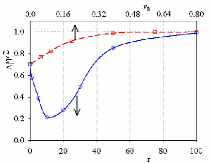
Figure 2. A fraction of electron density localized on the polaron Δ|Ψ|2 as function of switching-on time τ (solid line, open circles); Δ|Ψ|2vs initial polaron velocity v
0 (dashed line, open squares) at instant field switching-on; χ = 0.4.
If at first the field increases linearly (B = Bmaxt/τ for t ≤ τ
and B = Bmax for t > τ), then the fraction of the electron
density Δ|Ψ|2 left at the polaron depends on τ
nonmonotonically. The result is shown in figure 2 (solid curve and circles). Here, Bmax = 0.08, χ = 0.4, and the initial
charge leaves the polaron, it remains stable. But in this case its amplitude decreases, and the width increases because of the renormalization of the wave function on the polaron. Similar polaron behavior is observed for χ = 1.2. However, in this case the polaron is more "compact" (it has a smaller width and a larger amplitude), the wave function is better attached to the polaron, and the polaron itself is more stable to the variation of the initial conditions.
Thus, figure 2 demonstrates the closer the initial conditions correspond to the stationary state of the polaron, the faster and more "confident" the polaron reaches this stationary, while maintaining the complete norm of the wave function. In all numerical simulation, only such initial conditions are used below, which provide at least 99 % localization of the wave function density at the polaron.
Stationary polaron velocity
Numerical simulations reveal that the relations between polaron parameters (amplitude, velocity, width) do not depend on the presence of the electric field. That is, the field initially only accelerates the polaron, and after that it moves at a constant velocity as if without the field. The influence of the electric field is discussed in more detail below.
Figure 3. Amplitude of relative displacements A vs polaron velocity v without electric field (solid line is analytics83) and in electric field (circles, numerical simulation); χ = 0.4
Figure 3 shows the relation between the amplitude and the velocity of the polaron in the electric field and without the field for the EPI parameter χ = 0.4. Circles in figure 3corresponds to data in Figure 1 when the polaron accelerates in electric field of different values. For larger values of χ, e.g. χ = 1.2, the continual approximation is not applicable because the corresponding polaron is narrow. However, as the polaron with χ = 1.2 is much more stable in the electric field and quickly reaches the stationary state, the initial values of the polaron parameters are less significant. And it is reasonable to set initial conditions according to eqn. (6), choosing polaron parameters so that at least 99 % of the wave function density is localized at the polaron during the further evolution. In this case the wave function is the lowest-energy eigenfunction at the Hamiltonian diagonalization (eqn. 3).
The dependence of the steady-state velocity on the field strength B is weakly logarithmic. Figure 4 demonstrates less
than 10 % difference in stationary polaron velocities within four orders of magnitude of the field strength. Therefore, in polyacetylene and DNA, the stationary polaron velocity slightly depends on the applied electric field. The small polaron velocity in very low field can be explained by the fact that the polaron has not yet reached a stationary state during the numerical simulation (t ≤ 10000). Note, the dependences in Figure 4 are in good agreement with the dependences of the polaron velocity on the applied field.80
Figure 4. Stationary polaron velocity vvs electric field parameter
B for χ = 1.2 (dashed line and squares) and χ = 0.4 (solid line and circles). The dimensionless velocity is measured in units of sound velocities. The inset shows dependencies in linear coordinates.
Generation of longitudinal coherent vibrations
The energy transferred from the electric field to the polaron, in general, can be used in several ways. First, this energy can be spent on accelerating the polaron and, accordingly, on increasing its kinetic energy. Secondly, energy can provide growth of potential energy due to a change in the polaron shape with an increase of the amplitude and a decrease of the width. Correspondingly, the electron energy changes due to the electron-phonon interaction. Finally, some of the energy can be transferred to lattice vibrations.
After the polaron reached a stationary state, the polaron continues to receive energy due to the interaction of the charge with the electric field. The constant power of this interaction is p = fvst, where f = eE (e is the polaron charge,
E is the electric field strength, vst is the stationary polaron
velocity). In this case, the total energy of the "polaron + external field" system grows linearly with time. Since the polaron self-energy does not change, all the power consumed is converted only into lattice vibrational energy. Thus, the polaron velocity is determined by the balance of energies: the energy gained by the polaron in the electric field should be equal to the energy dissipated into the lattice.
The two top panels of figure 5 show snapshots of particles relative displacements qj ≡ (xj+1- xj) for χ = 0.4 (left top
because they are generated during the field switching-on period. Region b can cover several thousand lattice periods and represents coherent oscillations. (Figure 6.)
The time dependence of chosen bond q500 = x501 - x500
oscillations is shown in Figure 6. Polaron passes the bond at
t = 762. After this, the bond oscillates with constant frequency and amplitude. The apparent amplitude modulation is due to the incommensurability of the oscillations period and the period of the particle displacement measurement, as illustrated in the inset to the figure.
Figure 5. Snapshots of the relative displacements qj at the time t. Upper row: polaron on the harmonic lattice in electric field. The left
upper panel: χ = 0.4, v0 = 0.8, B = 0.1, t = 2250. The right upper panel: χ = 1.2, v0 = 0.65, B = 1.0, t = 2825. In both cases, the polaron was initially located at j0 = 2500 and the field switching-on rate is c = 1/1250. Polarons are centered at j = 4380 and j = 4420 in the left and
right panels, respectively. Lower row: the "demon" model (see Section 3.5). The lower left panel: vd = 0.862, t = 2320. The right lower panel vd = 0.617, t = 2430. In both cases, the excitation is initially localized at j0 = 2500.
Figure 6. Relative displacement q500 vs time, χ = 1.2. The inset illustrates the incommensurability of the true oscillations period (dashed line) and the period of numerical calculation (solid line).
Both space and time Fourie spectra have one peak corresponding to the wave number k (the wavelength
λ = 2π/k), and frequency ω of the generated oscillations, respectively. Thus, moving polaron generates stable coherent oscillations described by the equation
qj = C sin(kj + ωt + φ), where φ is the phase. The values of k
and ω are determined by the polaron velocity and the amplitude is determined by the applied field strength, which is in agreement with the reported value.80 The dependence of
k and ω on polaron velocity is discussed below.
Spectral characteristics of generated coherent vibrations
In the previous section, it was shown that the generated vibrations have definite values of k and ω. Because of the
fact that the field parameter B is uniquely related with the stationary polaron velocity (Figure 3), it is convenient to depict the spectral characteristics k and ω through the stationary polaron velocity v. These dependences are shown in figure 7.
Figure 7. Dependences of the wave number k (upper curve and symbols) and the frequency ω (lower curve and symbols) on the polaron velocity for χ = 1.2 (empty squares) and χ = 0.4 (empty circles) and on the "demon" velocity (filled triangles). Symbols for the wave number refer to the left axis, and symbols for the frequency refer to the right axis.
for χ=1.2 in the velocity range 0.55≤v≤0.62 (empty squares
in Figure 7). The character of k versus v dependences is different. The wave number increases with increasing speed for χ = 1.2 (empty squares), and decreases for χ = 0.4 (empty circles). The wavelength of the shortest-wave "optical" mode on the harmonic lattice is λ = 2 in the lattice constants, which corresponds to k = π. This means that for χ = 1.2 the polaron excites the shortest-wave mode with λ ≈ 2.2. For
χ = 0.4, the wavelength of the excited oscillations is slightly larger and λ ≈ 3.1.
The oscillations frequencies are also not very different. The steps-like dependence of ω in Figure 7 is due to the finite value of the integration step. The decrease of the step increases the smoothness of the dependence of ω vs v. In dimensional units, the oscillation frequency is ≈ 2 1012 Hz
at the polaron velocity v = 0.57 (χ = 1.2, DNA), and the frequency is ≈ 3 1013 Hz at the polaron velocity v = 0.86
(χ = 0.4, PA).
It was shown80 that the wave number k depends on the
polaron velocity v and it is determined by the following equation (mod 2π), where vsnd is the sound velocity and the
frequency is determined by the dispersion equation
𝜈𝑘 = 𝜈snd sin(𝑘 2⁄ ) (8)
𝜛𝑘= 𝜈snd |sin(𝑘 2⁄ )| (9)
Our results are in good agreement with eqns. (8) and (9). Indeed, for v = 0.8 and v = 0.65 these equations give k ≈ 2.3,
ω ≈ 1.8 and k ≈ 3.1, ω ≈ 2.0, respectively. These points fit well in figure 7.
"Demon" Model
As shown above, the moving polaron generates coherent vibrations, and the wave number and the frequency of these vibrations are determined by the applied field (or the polaron velocity). One can say that the polaron is an effective "generator" of stable coherent lattice vibrations, and thousands of lattice sites can participate in these oscillations.
The polaron velocities fall in a narrow range of values (0.56≤v≤0.62 and 0.82≤v≤0.86 for DNA and PA,
respectively). It is a question, whether generation of such oscillations is possible in some other way than by localized moving compression of special shape. If possible, what are the spectral characteristics of these oscillations over a wider range of velocities of the generating source, and what should be the profile of the generative force.
In light of these questions, eqn. (8) deserves special attention. The fact is that eqn. (4) can be rewritten as d2x
j/dt2 = - (2xj - xj+1- xj-1) + fj(t), where fj(t) is a generic
force. The force has a profile of a moving impulse, while the profile itself can be of arbitrary shape. In this case, the wave number is determined from the eqn. (8), and the frequency from the dispersion law (eqn. 9).
We propose a simple model called "demon". This is a dynamic model of the compression moving on harmonic lattice in the absence of EPI. The compression has a step-like shape with a width of one lattice period. The power
transferred to the lattice is constant in time and depends on the deformation value. In this model, the demon velocity can vary within 0 < vd < 1, which is out of the limits of polaron
velocities for two EPI parameters under consideration. We consider the "demon" velocity varying in the range 0.55 ≤ vd ≤ 0.9.
Two lower panels of figure 5 show snapshots of the relative displacements in the harmonic lattice with moving "demon". Comparison of upper and lower panels demonstrates that the oscillations generated by "demon" are very similar to those generated by polaron moving with the same velocity.
Analysis of the spectral characteristics of the generated oscillations shows that the "demon" and the polaron moving with the same velocity excite oscillations with the same wave numbers and frequencies. In figure 7, the frequency and the wave number in the "demon" model are shown by filled triangles. It is seen that in the ranges of polaron velocities, the dependencies for the "demon" model and for polaron in electric field completely coincide. In this case, the wave numbers obey eqn. (8), and the frequencies are calculated from eqn. (9).
Eqn. (8) has a simple physical meaning. For all values of polaron velocity, the equation has one solution which is in the range 0 ≤ k ≤ 2π, and this solution corresponds to the wave with phase velocity equal to the velocity of the generating source (vphase = ω/k). It is obvious from
combination of eqns. (8) and (9). For small velocities (v ≤ 0.13), eqn. (8) has more than one solutions. For
example, for v = 0.1 there are three solutions, k1 = 5.705,
k2 = 14.136, and k3 = 16.846. One can easily check that all
three waves with corresponding wave numbers are presented in the Fourie spectra of vibrations generated by "demon" moving with v = 0.1.
Critical electric field
The equations of motion (4) and (5) do not imply any limitation on value of electric field. Really, we did not find a maximum field in the range of reasonable values if appropriate initial conditions are chosen, in particular the field switching-on rate is rather low. The situation drastically changes if the field is switch on instantaneously, and it is the instantaneous field switching-on has a physical sense.
The theoretical estimation of critical field has been reported.80 Estimations are based on the fact that, when the
large field is switched on instantly, a tilted potential is formed. The heavy and slow lattice does not have time to readjust. However, the electron can tunnel through the potential.
The critical field is defined as a field, when the probability of tunneling per unit time Γtun is of the same order of
magnitude as the reciprocal of the lattice readjusting time,
Γlat. For analytical estimations the triangular barrier is
considered. Then the tunnelling probability can be estimated by the WKB method.84 In the case of initial standing polaron
𝛤tun= 4exp [− 4𝑒b3 2⁄
3𝑡01 2⁄𝑒𝐸𝑎] (10)
The lattice readjusting time is estimated as the time necessary for the sound to pass a distance equal to the sum of the polaron width and the barrier width. Then Γlat has the
form
𝛤lat=
𝜈snd
𝑒b⁄𝑒𝐸𝑎+1 𝜒⁄ 2 (11)
The critical field can be estimated as
𝛤lat= 𝛤tun (12)
Since the tunnelling has a physical meaning in the continuum limit the above relations are true when the continuum approximation works, i.e. for sufficiently small χ. As we have already noted, χ = 0.4 is the limiting value of the electron-phonon interaction, when the continuum approximation is well applicable. So we can expect an agreement between analytical and numerical estimations of critical field. For χ = 0.4, eqns. (10)-(12) give values
Ecr ≈ 0.00071 in dimensionless units, which corresponds to
Bcr = eaEcr /ħ ≈ 0.076.
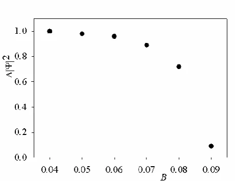
In numerical experiment we determine the fraction of electron density remaining on the polaron Δ|Ψ|2 if the field
is switched on instantly in the case of initial standing polaron (see figure 8). For field upto B ≈ 0.04, almost 100 % of electron density is localized at the polaron. For higher values of B, Δ|Ψ|2 drastically decreases. We define the
critical field as a field at which about 90 % of the total electron density remains on the polaron. Then numerical experiment gives Bcrnum ≈ 0.07, which is in good agreement
with analytical estimation. This value corresponds to 4.7·107
V/m in dimension units. (Figure 8)
Figure 8. A fraction of electron density localized on the polaron Δ|Ψ|2 after the instantaneous switching-on of the electric field vs field parameter B; χ = 0.4.
In the case of χ = 1.2, we can hardly expect such a coincidence between theoretical prediction and numerical results, because for large values of χ, the continuum
approximation does not work. However, some estimations can be done. For χ = 1.2, the manually fitted parameters are
A ≈ 0.78 and d ≈ 0.7 for standing polaron and the numerically calculated barrier height (the electronic part of the polaron coupling energy) is about 0.96. Then equations (10)-(12) give the magnitude of the critical field parameter
B1.2cr ≈ 18. This value is slightly higher than those estimated
numerically B1.2num ≈ 13. However, taking into account that
equations (10)-(12) are derived in an approximation that does not work for χ = 1.2, such a coincidence is surprising. Note, B1.2num corresponds to 2·108 V/m for DNA.
CONCLUSIONS
Polarons on harmonic lattice with EPI parameter corresponding PA and DNA are very stable in a constant electric field.
The results of the numerical simulation are rather sensitive to the initial conditions and to the method of switching-on the electric field. The main criterion of the simulation correctness is the complete localization of the electron density on the polaron. With unsuccessful initial conditions, a part of the electron density decouples from the lattice deformation. In all presented results at least 99 % of the total electron density is localized on the polaron. In the case of complete localization of the electron density on the polaron, the results do not depend on the initial conditions and the method of switching-on the electric field.
The polaron moves with constant velocity in electric field. The dependence of the stationary velocity on the applied field is weakly logarithmic. Within four orders of magnitude of the field strength, stationary velocities vary ≤ 10 %. This means that in polyacetylene and DNA the dependence of the polaron velocity on the applied electric field is insignificant.
The parameters (amplitude, width, velocity) of a stationary moving polaron in an electric field coincide with the parameters of a polaron moving with the same velocity in the absence of an electric field, which indicates the adiabatic polaron movement.
Polaron moving in electric field generates coherent oscillations. The spectral characteristics of the generated oscillation are well described by a simple ''demon'' model. This means that any moving localized excitation of arbitrary shape generates coherent oscillations of the harmonic lattice. The phase velocity of generated oscillations is equal to the polaron/"demon" velocity.
For appropriate initial conditions, i.e. adiabatically slow field switching-on rate or initially moving polaron, we did not find maximum value of the electric field resulting in polaron destruction. However, in the case of instantaneous field switching-on, rather low fields destroy initially standing polaron. The estimated values of critical field are 4.7·107 V m-1 and 2·108 Vm-1 for polyacetylene and DNA,
respectively.
References
1Friedman, K. A., Heller, A., On the Non-Uniform Distribution of Guanine in Introns of Human Genes: Possible Protection of Exons against Oxidation by Proximal Intron Poly-G Sequences, J. Phys. Chem. B, 2001, 105, 11859. DOI: 10.1021/jp012043n
2Endres, R. G., Cox D. L., Singh R. R. P., The quest for high-conductance DNA, Rev. Mod. Phys., 2004, 76, 195. DOI: 10.1103/RevModPhys.76.195
3Fink, H.-W., Schonenberger, Ch., Electrical conduction through DNA molecules, Nature, 1999, 398, 407. DOI:10.1038/18855
4Porath, D., Bezryadin, A., de Vries, S., Dekker, C., Direct measurement of electrical transport through DNA molecules,
Nature, 2000, 403, 635. DOI:10.1038/35001029
5Genereux, J. C., Barton, J. K., Mechanisms for DNA Charge Transport, Chem. Rev., 2010, 110, 1642. DOI: 10.1021/cr900228f
6Genereux, J. C., Wuerth, S. M., Barton, J. K., Single-Step Charge Transport through DNA over Long Distances,, J. Am. Chem. Soc., 2011, 133, 3863. DOI: 10.1021/ja107033v
7Arikuma, Y., Nakayama, H., Morita, T., Kimura, S., Electron Hopping over 100 Å Along an α Helix, Angew. Chem. Int. Ed., 2010, 49, 1800. DOI: 10.1002/anie.200905621
8Augustyn, K. E., Genereux, J. C., Barton, J. K., Distance‐ Independent DNA Charge Transport across an Adenine Tract,
Angew. Chem. Int. Ed., 2007, 46, 5731. DOI: 10.1002/anie.200701522
9Barton J. K., Olmon E. D., Sontz, P. A., Metal Complexes for DNA-Mediated Charge Transport, Coordin. Chem. Rev.,
2011, 255, 619. DOI: 10.1016/j.ccr.2010.09.002
10Slinker, J. D., Muren, N. B., Renfrew, S. E., Barton, J. K., DNA charge transport over 34 nm, Nat. Chem., 2011, 3, 228. DOI:10.1038/nchem.982
11Cordes, M., Giese, B., Electron transfer in peptides and proteins,
Chem. Soc. Rev., 2009, 38, 892. DOI: 10.1039/B805743P
12Astakhova, T. Yu., Likhachev, V. N., Vinogradov, G. A., Long-range charge transfer in biopolymers, Russ. Chem. Rev., 2012,
81, 994. DOI: 10.1070/RC2012v081n11ABEH004308
13Su, W. P., Schrieffer, J. R., Heeger, A. J., Solitons in Polyacetylene, Phys. Rev. Lett., 1979, 42, 1698. DOI: 10.1103/PhysRevLett.42.1698
14Su, W. P., Schrieffer, J. R., Heeger, A. J., Soliton excitations in polyacetylene, Phys. Rev. B, 1980, 22, 2099. DOI: 10.1103/PhysRevB.22.2099
15Su, W. P., Schrieffer, J. R., Soliton dynamics in polyacetylene,
Proc. Natl. Acad. Sci. USA, 1980, 77, 5626. DOI: 10.1073/pnas.77.10.5626
16Su, W. P., Schrieffer, J. R., Fractionally Charged Excitations in Charge-Density-Wave Systems with Commensurability 3,
Phys. Rev. Lett., 1981, 46, 738. DOI:
10.1103/PhysRevLett.46.738
17Takayama, H., Lin-Liu, Y. R., Maki K., Continuum model for solitons in polyacetylene, Phys. Rev. B, 1980, 21, 2388. DOI: 10.1103/PhysRevB.21.2388
18Wilson, E. G., J. Phys. C, A new theory of acoustic solitary-wave polaron motion, 1983, 16, 6739. DOI: 10.1088/0022-3719/16/35/008
19Arikabe Y., Kuwabara, M., Ono, Y., Dynamics of an Acoustic Polaron in One-Dimensional Electron-Lattice System, J. Phys. Soc. Jpn., 1996, 65, 1317. DOI: 10.1143/jpsj.65.1317
20Marcus, R. A., Electron Transfer Reactions in Chemistry: Theory and Experiment, Angew. Chem., Int. Edit., 1993, 32, 1111. DOI: 10.1002/anie.199311113
21Sartor, V., Boone, E., Schuster, G. B., Long-Distance Radical Cation Migration through A/T Base Pairs in DNA: An Experimental Test of Theory, J. Phys. Chem. B, 2001, 105, 11057. DOI: 10.1021/jp011354v
22Meggers, E., Michel-Beyerle, M. E., Giese, B., Sequence Dependent Long Range Hole Transport in DNA, J. Am. Chem. Soc., 1998, 120, 12950. DOI: 10.1021/ja983092p
23Conwell, E. M., Rakhmanova, S. V., Polarons in DNA, Proc.
Natl. Acad. Sci. USA, 2000, 97, 4556. DOI: 10.1073/pnas.050074497
24Rakhmanova, S. V., Conwell, E. M., Polaron Motion in DNA, J.
Phys. Chem. B, 2001, 105, 2056. DOI: 10.1021/jp0036285 25Conwell, E. M., Basko, D. M., Hole Traps in DNA, J. Am. Chem.
Soc., 2001, 123, 11441. DOI: 10.1021/ja015947v
26Conwell, E. M., Charge transport in DNA in solution: The role of polarons, Proc. Natl. Acad. Sci., 2005, 102, 8795. DOI: 10.1073/pnas.0501406102
27Komineas, S., Kalosakas, G., Bishop, A. R., Effects of intrinsic base-pair fluctuations on charge transport in DNA, Phys. Rev. E, 2002, 65, 061905. DOI: 10.1103/PhysRevE.65.061905 28Kalosakas, G., Rasmussen, K. O., Bishop, A. R., Charge trapping
in DNA due to intrinsic vibrational hot spots, J. Chem. Phys.,
2003, 118, 3731. DOI: 10.1063/1.1539091
29Chang, C.-M., Castro Neto, A. H., Bishop, A.R., Long-range charge transfer in periodic DNA through polaron diffusion,
Chem. Phys., 2004, 303, 189. DOI:
10.1016/j.chemphys.2004.05.015
30Berashevich, J. A., Bookatz, A. D., Chakraborty, T., The electric field effect and conduction in the Peyrard–Bishop–Holstein model, J. Phys.- Condens. Mat., 2008, 20, 035207. DOI: 10.1088/0953-8984/20/03/035207
31Berashevich, J. A., Chakraborty, T., Electronic parameters for the hole transfer in DNA duplex oligomers, Chem. Phys. Lett.,
2007, 446, 159. DOI: 10.1016/j.cplett.2007.08.045
32Hawke, L. G. D., Kalosakas, G., Simserides, C., Electronic parameters for charge transfer along DNA, Eur. Phys. J. E,
2010, 32, 291. DOI: 10.1140/epje/i2010-10650-y
33Yamada, H., Starikov, E. B., Hennig, D., Quantum diffusion in polaron model of poly(dG)-poly(dC) and poly(dA)-poly(dT) DNA polymers, Eur. Phys. J. B, 2007, 59, 185. DOI: 10.1140/epjb/e2007-00274-4
34Kalosakas, G., Charge transport in DNA: Dependence of diffusion coefficient on temperature and electron-phonon coupling constant, Phys. Rev. E, 2011, 84, 051905. DOI: 10.1103/PhysRevE.84.051905
35Kucherov, V. M., Kinz-Thompson, C. D., Conwell, E. M., Polarons in DNA Oligomers, J. Phys. Chem. C, 2010, 114, 1663. DOI: 10.1021/jp908809t
36Qu Z., Kang, D. W., Jiang, H., Xie, S. J., Temperature effect on polaron dynamics in DNA molecule: The role of electron-base interaction, Physica B, 2010, 405, S123. DOI: 10.1016/j.physb.2009.12.020
37Triberis, G., Simserides, C., Karavolas, V., A small polaron hopping model for multiphonon-assisted transport along DNA molecules,in the presence of disorder, Physica E, 2006,
32, 592. DOI: 10.1016/j.physe.2005.12.111
38Cuniberti, G., Fagas, G., Richter, K., Fingerprints of mesoscopic leads in the conductance of a molecular wire, Chem. Phys.,
2002, 281(2-3), 465. DOI: 10.1016/S0301-0104(02)00341-5
39Todorov, T. N., Tight-binding simulation of current-carrying nanostructures, J. Phys.-Condens. Mat., 2002, 14(11), 3049. DOI: 10.1088/0953-8984/14/11/314
41e Silva, G. M., Electric-field effects on the competition between polarons and bipolarons in conjugated polymers, Phys. Rev. B, 2000, 61, 10777. DOI: 10.1103/PhysRevB.61.10777
42Peng, C., Jian, W., GuiQing, Zh., ChengBu, L., Hole polarons in poly(G)-poly(C) and poly(A)-poly(T) DNA molecules, Sci. China Ser. B, 2008, 51, 1182. DOI: 10.1007/s11426-008-0128-y
43Basko, D. M., Conwell, E. M., Self-trapping versus trapping: Application to hole transport in DNA, Phys. Rev. E, 2002, 65, 061902. DOI: 10.1103/PhysRevE.65.061902
44Zheng, B., Wu, J., Sun, W., Liu, Ch., Trapping and hopping of polaron in DNA periodic stack, Chem. Phys. Lett, 2006, 425, 123. DOI:10.1016/j.cplett.2006.05.022
45Lin, X., Li, J., Smela, E., Yip, S., Polaron‐induced conformation change in single polypyrrole chain: An intrinsic actuation mechanism, Int. J. Quantum Chem., 2005, 102, 980. DOI: 10.1002/qua.20433
46Falleiros, M. B., e Silva, G. M., Polaron and bipolaron stability on paraphenylene polymers, J. Mol. Model., 2017, 23, 59. DOI: 10.1007/s00894-017-3215-1
47Ma, H., Schollwock, U., Dynamical simulations of polaron transport in conjugated polymers with the inclusion of electron-electron interactions, J. Phys. Chem. A, 2009, 113(7), 1360. DOI: 10.1021/jp809045r
48Ribeiro, L. A., da Cunha, W. F., de O. Neto, P. H., Gargano, R., e Silva, G. M., Effects of temperature and electric field induced phase transitions on the dynamics of polarons and bipolarons, New J. Chem., 2013, 37, 2829. DOI: 10.1039/c3nj00602f
49Hultell, M., Stafstrom, S., Polaron dynamics in highly ordered molecular crystals, Chem. Phys. Lett., 2006, 428, 446. DOI:10.1016/j.cplett.2006.07.042
50Johansson, A., Stafstrom, S., Polaron Dynamics in a System of Coupled Conjugated Polymer Chains, Phys. Rev. Lett., 2001,
86, 3602. DOI: 10.1103/PhysRevLett.86.3602
51Johansson, A., Stafstrom, S., Soliton and polaron transport in
trans-polyacetylene, Phys. Rev. B, 2002, 65, 045207. DOI: 10.1103/PhysRevB.65.045207
52Alexandrov, A. S., Yavidov, B. Ya., Small adiabatic polaron with a long-range electron-phonon interaction, Phys. Rev. B, 2004,
69, 073101. DOI: 10.1103/PhysRevB.69.073101
53Diaz, E., Lima, R. P. A., Dominguez-Adame, F., Bloch-like oscillations in the Peyrard-Bishop-Holstein model, Phys. Rev. B, 2008, 78, 134303. DOI: 10.1103/PhysRevB.78.134303
54Hague, J. P., Kornilovitch, P. E., Alexandrov, A. S., Samson, J. H., Effects of lattice geometry and interaction range on polaron dynamics, Phys. Rev. B, 2006, 73, 054303. DOI: 10.1103/PhysRevB.73.054303
55Mozafari, E., Stafstrom, S., Polaron dynamics in a two-dimensional Holstein-Peierls system, J. Chem. Phys., 2013,
138, 184104. DOI: 10.1063/1.4803691
56Wei, J. H., Liu, X. J., Berakdar, J., Yan, YiJing, Pathways of polaron and bipolaron transport in DNA double strands, J. Chem. Phys., 2008, 128, 165101. DOI: 10.1063/1.2902279
57Luo, J., Piette, B. M. A. G., A generalised Davydov-Scott model for polarons in linear peptide chains, Eur. Phys. J. B, 2017,
90, 155. DOI: 10.1140/epjb/e2017-80209-2
58Hennig, D., Neibner, C., Velarde, M. G., Ebeling, W., Effect of anharmonicity on charge transport in hydrogen-bonded systems, Phys. Rev. B, 2006, 73, 024306. DOI: 10.1103/PhysRevB.73.024306
59da Cunha, W. F., Neto, P. H. de O., Gargano, R., e Silva, G. M., Temperature effects on polaron stability in polyacetylene, Int. J. Quantum Chem., 2008, 108, 2448. DOI: 10.1002/qua.21798
60Zhang, Y. L., Liu, X. J., An, Z., Temperature dependence of polaron stability in conjugated polymers, Europhys. Lett,
2015, 111, 17009. DOI: 10.1209/0295-5075/111/17009
61Yao, Y., Qiu, Y., Wu, Ch.-Q., Dissipative dynamics of charged polarons in organic molecules, J. Phys.- Condens. Matter,
2011, 23, 305401. DOI: 10.1088/0953-8984/23/30/305401
62Ojeda J. H., Lima, R. P. A., Dominguez-Adame, F., Orellana, P. A., Trapping and motion of polarons in weakly disordered DNA molecules, J. Phys.- Condens. Matter, 2009, 21, 285105. DOI:10.1088/0953-8984/21/28/285105
63Zhang, G., Cui, P., Wu, J., Liu, Ch., Structural fluctuation effect on the polaron in DNA, Physica B, 2009, 404, 1485. DOI:10.1016/j.physb.2009.01.004
64Yan, Y. H., An, Z., Wu, C.Q., Dynamics of polaron in a polymer chain with impurities, Eur. Phys. J. B, 2004, 42, 157. DOI: 10.1140/epjb/e2004-00367-6
65Wang, Y. D., Zhang, X. G., Meng, Y., Di, B., Zhang, Y. L., An, Z., Dynamic recombination of polaron pair with impurity in conjugated polymers, Org. Electron., 2017, 49, 286. DOI: 10.1016/j.orgel.2017.06.067
66Johansson, A, Stafstrom, S., Nonadiabatic simulations of polaron dynamics, Phys. Rev. B, 2004, 69, 235205. DOI: 10.1103/PhysRevB.69.235205
67Li, Y., Liu, X.-J., Fu, J.-Y., Liu, D-Sh., Xie, Sh.-J., Mei, L.-M., Bloch oscillations in a one-dimensional organic lattice, Phys.
Rev. B, 2006, 74, 184303. DOI:
10.1103/PhysRevB.74.184303
68Ono, Y., Terai, A., Motion of Charged Soliton in Polyacetylene Due to Electric Field, J. Phys. Soc. Jpn., 1990, 59, 2893. DOI: 10.1143/JPSJ.59.2893
69Liu, X., Gao, K., Fu, J., Li, Y., Wei, J., Xie, Sh., Effect of the electric field mode on the dynamic process of a polaron, Phys.
Rev. B, 2006, 74, 172301. DOI:
10.1103/PhysRevB.74.172301
70Zhang, G., Hu, H., Cui, S., Lv, Z., Higher order tight binding Su– Schrieffer–Heeger method and its applications in DNA charge transport, Physica B, 2010, 405, 4382. DOI:10.1016/j.physb.2010.07.047
71Thornber, K. K., Feynman, R. P., Velocity Acquired by an Electron in a Finite Electric Field in a Polar Crystal, Phys. Rev. B, 1970, 1, 4099. DOI: 10.1103/PhysRevB.1.4099
72Ribeiro, L. A., da Cunha, W. F., Fonseca, A. L. de A., e Silva, G. M., Bloch oscillations in organic and inorganic polymers, J. Chem. Phys., 2017, 146, 144903. DOI: 10.1063/1.4979950
73da Silva, M. V. A., Neto, P. H. de O., Cunha, W. F. da, Gargano, R., e Silva, G. M., Supersonic quasi-particles dynamics in organic semiconductors, Chem. Phys. Lett., 2012, 550, 146. DOI: 10.1016/j.cplett.2012.09.012
74Rakhmanova, S. V., Conwell, E. M., Polaron dissociation in conducting polymers by high electric fields, Appl. Phys. Lett.,
1999, 75, 1518. DOI: 10.1063/1.124741
75Rakhmanova, S. V., Conwell, E. M., Nonlinear dynamics of an added carrier in trans-polyacetylene in the presence of an electric field, Synthetic Met., 2000, 110, 37. DOI: 10.1016/S0379-6779(99)00261-1
76Mahani, M. R., Mirsakiyeva, A., Delin, A., Breakdown of Polarons in Conducting Polymers at Device Field Strengths,
Phys. Chem. C, 2017, 121, 10317. DOI:
10.1021/acs.jpcc.7b02368
77Yu, J. F., Wu, C. Q., Sun, X., Nasu, K., Breather in the motion of a polaron in an electric field, Phys. Rev. B, 2004, 70, 064303. DOI: 10.1103/PhysRevB.70.064303
79Nazareno, H. N., de Brito, P. E., Bloch oscillations as generators of polarons in a 1D crystal, Physica B, 2016, 494, 1. DOI: 10.1016/j.physb.2016.04.029
80Basko, D. M., Conwell, E. M., Stationary Polaron Motion in a Polymer Chain at High Electric Fields, Phys. Rev. Lett.,
2002, 88, 056401. DOI: 10.1103/PhysRevLett.88.056401
81Likhachev, V. N., Astakhova, T. Yu., Vinogradov G.A., Поляроны в одномерной решетке. I. Неподвижный поляронRuss. Khim. Fiz., 2013, 32, 3. DOI: 10.7868/S0207401X13040092
82Carstea, A. S., Integrable systems related to Su-Schrieffer-Heeger lattices, Chaos Soliton Fract, 2009, 42, 923. DOI: 10.1016/j.chaos.2009.02.034
83Astakhova, T. Yu., Likhachev, V. N., Vinogradov, G. A., Polaron on a one-dimensional lattice: II. A moving polaron,
Russ. J. Phys. Chem. B, 2013, 7, 521. DOI: 10.1134/S199079311305028X
84Landau, L. D., Lifshitz, E. M., Quantum Mechanics,
Non-relativistic Theory, Second edition, revised and enlarged, Pergamon Press, 1965, 174-175.
85Landau, L. D., Lifshitz, E.M., Quantum Mechanics,
Non-relativistic Theory, Second edition, revised and enlarged, Pergamon Press, 1965, 72-73.