Sharif University of Technology
Scientia IranicaTransactions E: Industrial Engineering www.scientiairanica.com
A two-echelon inventory model with perishable items
and lost sales
A. Mahmoodi
, A. Haji and R. Haji
Department of Industrial Engineering, Sharif University of Technology, Tehran, Iran. Received 4 May 2014; received in revised form 7 May 2015; accepted 6 September 2015
KEYWORDS Inventory; Perishable items; Base stock policy; Lost sales; Two-echelon.
Abstract.This article deals with a single perishable item, continuous-review, two-echelon serial inventory system consisting of a warehouse and a retailer. Customer demands at the retailer are assumed to be Poisson. All items have a xed shelf life and start aging on their arrival at the retailer. The demand that cannot be met immediately at the retailer is lost. All transportation times are xed. If there is any stock in the warehouse, the lead time for the retailer would be the transportation time from the warehouse. Otherwise, the retailer orders are met with a delay. In this article, using an approximate technique, we rst present a heuristic for nding cost-eective base stock policy and then develop a simulation-based neighborhood search procedure to modify the quality of the solution. Also, a numerical experiment is carried out to evaluate eectiveness and accuracy of the procedures. The results reveal that the approximate model performs rather well.
© 2016 Sharif University of Technology. All rights reserved.
1. Introduction
Most conventional inventory models are presented to deal with nonperishable items. However, perishable inventories are the major concern in many industrial sectors. Foodstus, pharmaceuticals, blood and its derivatives, batteries, and photographic lms are a few examples of perishable inventories. By disregarding the nite lifetime of perishable items, the resulting model may give inaccurate results. Therefore, lifetime of the item has to be taken into consideration to develop a cost-eective inventory model.
In this article, a single perishable item, continuous-review, two-echelon serial inventory system consisting of a warehouse and a retailer is considered. The retailer faces Poisson demand and replenishes its stock from the warehouse. The warehouse, in turn, replenishes its stock through an external supplier. The transportation time from the warehouse to the retailer
*. Corresponding author. Tel.: +98 21 66165704; Fax: +98 21 66022702
E-mail address: a [email protected] (A. Mahmoodi)
is xed. If there is any stock in the warehouse, the lead time for the retailer would be the transportation time. Otherwise, the retailer orders are met with a delay. The lead time on a warehouse order is xed. After joining the stock at retailer, an item has a constant shelf life, beyond which it is no longer usable. The demand that cannot be met immediately at the retailer is lost. The xed ordering cost is negligible and both installations operate base stock policy to control their inventories.
To the best of our knowledge, the papers which study perishable items in multi-echelon inventory sys-tems are very few. The optimal replenishment policies for a single perishable item, two-echelon inventory system were analyzed by Abdel-Malek and Ziegler [1]. They assumed deterministic demand for their inventory system. The problem of periodic review ordering and issuing policies in a two-echelon inventory system under demand uncertainty was considered by Fujiwara et al. [2]. However, they assumed unique lifetime for each echelon.
Furthermore, the eect of product perishability on total cost of the system in a two-echelon inven-tory system was investigated by Kanchanasuntorn and
Techanitisawad [3]. They developed an approximate inventory model under periodic review policies assum-ing normal demand for retailers.
Moreover, Olsson [4] addressed a continuous-review, two-echelon serial inventory system with per-ishable items and developed an approximate technique for evaluation of base stock policies. Considering Pois-son demand for the downstream location, he assumed that the unsatised demand was backordered. Finally, Mahmoodi and Haji [5] developed (1; T ) policy for a two-echelon inventory system with perishable-on-the-shelf items.
From a modeling point of view, our model is re-lated to single-echelon models with continuous review. Signicant studies have been carried out for inven-tory control of single installations of perishable items. Schmidt and Nahmias [6] addressed a system with perishable items operating under (S 1; S) policy with lost sales, Poisson demand, outdating costs, purchase costs, and per unit per period holding costs. Perry and Posner [7] generalized Schmidt and Nahmias [6] to allow for general types of customer impatience behavior. Olsson and Tydesjo [8] extended Schmidt and Nahmias [6] by allowing backorders. Mahmoodi et al. [9] considered an inventory system under Schmidt and Nahmias [6] assumptions but employed (1; T ) policy instead of (S 1; S) policy. The interested reader can refer to [10] and [11], which are two comprehensive reviews focusing on inventory control of perishable items.
This paper presents an approach to deal with replenishment problem in a single perishable item, two-echelon inventory system under continuous review and lost sales. The considered inventory system in this paper is dierent from inventory systems studied in the literature. For example, our system is dierent from Abdel-Malek and Ziegler [1] in that we consider stochastic demand. Fujiwara et al. [2] and Kanchana-suntorn and Techanitisawad [3], unlike our continuous review, considered periodic review policies. Finally, although like Olsson [4] we consider continuous review, we assume lost sales.
For the items with innite lifetime, our model is reduced to the one considered by Andersson and Melchiors [12]. However, the inclusion of perishability requires an entirely new analysis due to the fact that not only the perished items aect the demand of the warehouse but also the retailer should make tradeo between the number of lost sales and the number of perished items.
Considering lost sales and perishable items, the demand process at the warehouse is not a Poisson process. We ignore this and approximate the demand process at the warehouse with a Poisson process. Then, the approximated long-run average total cost function of the inventory system is derived. Furthermore, two
procedures are presented to obtain the optimal or near-optimal solution. Our approach gives an approximate model which is quite simple and ecient from a computational point of view. Simulation results show that the performance is very good. Although a serial system is considered, the presented model could easily be extended to a distribution system with identical retailers.
An interesting application of our proposed model is to a situation where an operating equipment is sub-ject to both failures and routine maintenance, which was introduced as an application of (S 1; S) policy by Schmidt and Nahmias [6]. In particular, consider a facility with S1 similar operating machines. Each
machine has an engine which is subject to failure at random times. Any engine which has been in service for a xed time m without failure is also removed for maintenance. Each time an engine is removed for maintenance or repair, an order for replacement is made from a warehouse. The warehouse operates under (S0 1; S0) policy. The transportation time from the
warehouse to the facility is xed and known. If there is any stock in the warehouse, the lead time for the facility would be the transportation time. Otherwise, the facility orders are met with a delay. The lead time on a warehouse order is xed. The number of operating machines in the facility is as the inventory on hand in the retailer in the considered model. Our model can be used to determine not only the inventory position at the warehouse but also the xed interval of routine maintenance (see [6] for more details).
The proceeding parts of this paper are organized as follows: in Section 2, the considered model is described. In Section 3, the cost function of the system is approximated. Then, in Section 4, two procedures are introduced to nd the best policy for the model. Furthermore, a numerical analysis is carried out to evaluate accuracy and eectiveness of procedures in Section 5. Finally, the conclusion and future research are presented in Section 6.
2. Model description
We consider a single-item, two-echelon (two locations) serial inventory system consisting of a warehouse and a retailer. Customer demands occur only at the retailer according to a Poisson process. The xed ordering costs are negligible. Thus, we apply the base stock policy (one for one policy) with continuous review in both locations. That is, the retailer makes its orders to the warehouse under (S1 1; S1) policy, and the
warehouse makes its orders to an external supplier with innite supply under (S0 1; S0) policy, where S1 and
S0 are the inventory positions in the retailer and in
the warehouse, respectively. We consider perishable-on-the-shelf items; that is, items have a xed shelf life
and start aging on their arrival at the retailer. All transportation times are xed. All satised demands are met based on FIFO (First In First Out) policy. Although the demand not met at the retailer is lost, the unsatised demand at the warehouse is backordered. A xed penalty cost per lost sale and a xed penalty cost per perished item are incurred at the retailer. Items held in stock both at the warehouse and at the retailers incur holding costs per unit per time unit. Also, the warehouse pays a xed purchase cost per item. Therefore, shortage, perishing, and holding costs are incurred at the retailer, and purchasing and holding costs are incurred at the warehouse. The objective is to nd optimal values of S1 and S0 to minimize total
cost of the system. The following notations are used in the subsequent parts of the paper.
Model Parameters:
1 The customer demand rate;
Cost of a lost sale at the retailer; h0 Holding cost per unit per time unit at
the warehouse;
h1 Holding cost per unit per time unit at
the retailer;
p Cost of a perished item at the retailer; c Purchase cost per unit at the
warehouse;
The rate of perishing at the retailer; 0 Transportation time from the external
supplier to the warehouse; 1 Transportation time from the
warehouse to the retailer;
m The shelf life of the items at the retailer;
I0 Average on-hand inventory at the
warehouse;
I1 Average on-hand inventory at the
retailer;
B0 The average number of backorders at
the warehouse. Decision variables:
S0 Inventory position at the warehouse;
S1 Inventory position at the retailer.
Cost measures:
H0 Average total holding cost per time
unit at the warehouse;
H1 Average total holding cost per time
unit at the retailer;
Average total shortage cost per time unit at the retailer;
OC Average total perishing cost per time unit at the retailer;
PC Average total purchasing cost per time unit at the warehouse;
C0 Total cost rate at the warehouse;
C1 Total cost rate at the retailer;
TC Total cost rate of the system.
3. Cost evaluation
3.1. Preliminaries - single installation model Schmidt and Nahmias [6] consider a single perishable item, single-location inventory system operating under (S 1; S) policy with lost sales, Poisson demand, outdating costs, purchase costs, and per unit per period holding costs. The results of their model are used to obtain the cost function of the retailer in our model. Therefore, some key results of their model are presented in the following.
Let Xk, 1 k S, represent the elapsed time
since the order of the kth oldest item in the system was placed. That is, X1 is the time since the oldest item
was ordered, X2is the time since the second oldest item
was ordered, etc. Then, the joint density function of X1; :::; XS is stated as:
fX1;X2;:::;XS(x1; x2; :::; xS)
= (
Ke for x 1<
Ke x1 for x1
for x1 x2 ::: xS and S > 0;
where, and stand for the demand rate and the lead time, respectively. Also, K is a normalizing constant, which is obtained as:
K =
e S
S! + Z +m
xS 1e x
(S 1)! dx 1
: (1)
Also, using the marginal function of the oldest item, the rate of perishing is obtained (Eq. (7) in [6]):
= fX1( + m) =
Ke (+m)( + m)S 1
(S 1)! : (2) Furthermore, the proportion of time that the system is out of stock, P0, is:
P0=
Z
0
Z x1
0 :::
Z xS 1
0 Ke
dx
S:::dx1=Ke
S
S! :(3)
3.2. Approximate retailer cost
retailer orders an item, the lead time at the retailer is stochastic. That is, the replenishment lead time of the retailer is 1+ , where is the delay due to
stock-outs at the warehouse. We use the idea of the well-known METRIC model [13] and approximate the lead time by its mean. Thus, the lead time at the retailer is 0
1= 1+ , where is the mean of .
For a given 0
1, the retailer's model is quite
similar to the single installation model of Schmidt and Nahmias [6]. Therefore, by substitution of and with 0
1 and 1in Eq. (2), the perishing rate at the retailer
is:
= K0e 1(
0
1+m)(10+ m)S1 1
(S1 1)! ; (4)
where from Eq. (1):
K0 = e 1
0 110S1
S1! +
Z 0 1+m
0 1
xS1 1e 1x
(S1 1)! dx
! 1 :
(5) Thus, the perishing cost rate at the retailer is obtained as follows:
OC = p = pK0e 1(
0
1+m)(10+ m)S1 1
(S1 1)! : (6)
Furthermore, the proportion of time that the retailer is out of stock, P0, is obtained by substitution of and
with 0
1 and 1 in Eq. (3). Thus, P0 is:
P0= K
0e 1100
1S1
S1! : (7)
Since P0 is the proportion of time that the system is
out of stock, the proportion of demand that is lost is 1P0. Therefore, the shortage cost rate at the retailer
is:
= 1P0= 1K
0e 1100
1S1
S1! : (8)
Let L be the average number of outstanding orders towards the warehouse. Then, by Little's formula, L = W , where is the order rate and W is the time, an item is on order. In our case, W = 0
1 and = (1
P0)1+ , which gives L = 10((1 P0)1+ ). The
expected on hand inventory at the retailer is S1 L.
Thus:
I1= S1 L = S1 10((1 P0)1+ ) : (9)
Hence, the holding cost rate at the retailer is:
H1= h1I1= h1S1 h1101(1 P0) h110: (10)
Therefore, the total cost rate at the retailer can be
obtained from Eqs. (6), (8), and (10) as follows: C1= OC + + H1= (p h110)
K0e 1(10+m)(10+ m)S1 1
(S1 1)!
+( + h110)1K
0e 1100
1S1
S1! + h1S1 h1 0 11:
(11) 3.3. Approximate warehouse cost
Due to the existence of lost sales and perished items, the retailer demand to the warehouse is not Poisson. Like [12], we ignore this and approximate the demand at the warehouse with a Poisson process with mean 0= 1(1 P0) + .
Now, the number of outstanding orders towards the external supplier is as the occupancy level in an M=D=1 queue. According to Palm's theorem [14], for this type of queues, the steady-state occupancy level is Poisson distributed with mean L, where is the arrival rate and L is the mean service time. In our case, = 0, and L = 0. Hence, the average on hand
inventory and the average number of backorders at the warehouse are obtained as follows:
I0= S0
X
j=0
(S0 j)(00) j
j! e 00; (12)
B0= 1
X
j=S0+1
(j S0)(00) j
j! e 00: (13) Thus, the holding cost rate at the warehouse is:
H0= h0I0= h0 S0
X
j=0
(S0 j)(00) j
j! e 00: (14) Also, the average purchasing cost rate at the warehouse is:
PC = c0: (15)
Therefore, from Eqs. (14) and (15), the warehouse total cost rate is obtained as follows:
C0=PC+H0=c0+h0 S0
X
j=0
(S0 j)(00) j
j! e 00(16):
Furthermore, using Little's formula, the mean of delay at the retailer due to stock-outs at the warehouse, , can be obtained as follows:
= B0
Therefore, the replenishment lead time of the retailer is approximated as:
0
1= 1+B0
0: (18)
Finally, from Eqs. (11) and (16), total cost rate of the system can be obtained as follows:
TC =C0+ C1= c0+ h0 S0
X
j=0
(S0 j)(00) j
j! e 00
+ (p h110)K
0e 1(10+m)(0
1+ m)S1 1
(S1 1)!
+ ( + h110)1K
0e 1100
1S1
S1!
+ h1S1 h1101: (19)
4. Solution procedure
In Appendix A, we consider a base example and show that Eq. (19) is not convex over S0 and S1. Therefore,
in this section, we present a projection-based solution procedure, named Procedure 1, which constitutes a main loop and an inner loop. The main loop searches over the possible values of S0to nd the best one. For
each S0, an inner loop attempts to determine the best
values of S1. Evidently, S0 and S1cannot be negative
for a cost minimizing solution. Also, two lemmas are presented by which we can establish two termination criteria to bound S0 and S1 from above.
Lemma 1. Given a xed 0
1, the perishing rate at the
retailer, , is an increasing function of S1. Also ! 1
when S1! 1.
Proof. See Appendix B.
Lemma 2. For a xed 0, total cost rate of the
warehouse, C0, is a convex function of S0.
Proof. This lemma follows from, for example, [15] and [16].
The advantage of Procedure 1 is that with a temporary xed S0, we can use Lemma 1 to establish
a termination criterion for the inner loop. In more details, the search over S1 in inner loop can be
terminated when the perishing cost rate exceeds the best cost found for the retailer, that is when S1satises:
min
xS1C1(x) OC(S1) = p:
Furthermore, we can use Lemma 2 to construct a termination criterion for the main loop. Clearly, C0 is
a lower bound for TC. Therefore, since C0is convex in
S0, when S0 satises min
xS0TC(x) C0(S0), the search
over S0 can be terminated.
Procedure 1
- Step 0: Set S0:= 0, TCmin:= 1, S0opt:= 0, and
S1opt:= 0.
- Step 1: Set s := 0, S1:= 1, 10 := 1, TCS0min:=
1, and TCS1min:= 1. Calculate from Eq. (4)
and P0 from Eq. (7).
- Step 2: While TCS1min> p, do f
Calculate 0= 1(1 P0) + , 10 from Eq. (18) and
C1(S1; 10) from Eq. (11).
Calculate C0(S0; 0) from Eq. (16) and set
TC(S0) := C0(S0; 0) + C1(S1; 10).
If TC(S0) < TCS0min, then set TCS0min:= TC(S0),
:= 0, and s := S1.
If C1(S1) < TCS1min, then set TCS1min:= C1(S1).
Set S1:= S1+ 1.
Calculate from Eq. (4), and P0from Eq. (7).
g
- Step 3: Calculate C0(S0; ) from Eq. (16),
If TCS0min < TCmin then TCmin := TCS0min and
let S0opt:= S0 and S1opt:= s.
If TCmin < C
0(S0; ) then set S := (S0opt; S1opt),
return S and TCmin, and stop the procedure.
Otherwise, set S0:= S0+ 1 and go to Step 1.
When S0 = S1 = 0, all customer demands are
lost, which gives total cost of the system equal to 1.
Therefore, in Step 0 and Step 1, we can set all total cost rates to 1 as a starting point. Step 2 includes
the inner loop and search over S1. In Step 3, the
termination criterion of the main loop is checked and the procedure is continued or stopped, accordingly.
Due to the existence of 0
1and 0in cost functions,
and their dependence on both S0 and S1, with the
presented termination criteria, Procedure 1 may not obtain the optimal solution which minimizes approx-imated TC. However, numerical experiments show that in all considered problems this is not the case. In addition, the METRIC-based approximation for the retailer's lead time and Poisson approximation of the warehouse demand are used to obtain Eq. (19). Consequently, the optimal solution based on Eq. (19) is not necessarily the optimal solution of the inventory system. Therefore, apart from Procedure 1, we also propose Procedure 2, which is a neighborhood search based on simulation. In Procedure 2, for a given point S = (S0; S1), 8 neighborhoods including S =
(S0 1; S1), S = (S0+ 1; S1), S = (S0; S1 1), S =
(S0; S1+ 1), S = (S0 1; S1 1), S = (S0 1 + S1+1),
S = (S0 + 1; S1 1), and S = (S0+ 1; S1 + 1) are
10000 time units are executed. The average cost rate obtained from these 3 simulations is assigned to the corresponding neighborhood. If at least one improving solution has been determined, the neighborhood search is restarted with respect to the best of them. If no superior solution is found, the procedure stops and returns the best found solution. Procedure 2 starts with the obtained solution of Procedure 1.
We conjecture that there is a local optimum, which is also the global optimum. This conjecture is supported by all our numerical tests, yet we cannot for-mally prove it. Therefore, we consider two termination criteria for Procedure 2; rst, if no superior solution is found and, second, if the number of evaluated points exceeds a given upper bound Jmax. The latter never
occurs in our numerical analysis as we set Jmax = 50.
Thus, all nal solutions are local optimum according to the simulation.
Procedure 2
- Step 0: Set j := 1 and Jmax := 50. Execute
Procedure 1. Let S1 be the best policy found by
Procedure 1.
- Step 1: Execute 3 simulations with 10000 time units for Sj and set TCj to the average total cost rate
obtained by these simulations.
- Step 2: Execute 3 simulations with 10000 time units for all neighborhoods of Sj, which have not
been simulated before. Set Sj+1 to the policy
with the minimum average total cost rate among all neighborhoods. Also, set T Cj+1 to this total cost
rate.
- Step 3: If TCj+1< TCjand j J
max, set j := j+1
and go to Step 2. Otherwise, return to Sj as the
best policy and TCj as its total cost rate. Stop the
Procedure.
5. Numerical analysis
In this section, a small numerical study is performed to examine eectiveness and accuracy of the proposed procedures. In total, we consider 32 dierent test problems. We nd the best values of S0 and S1 for
each test problem according to Procedures 1 and 2. Then, eectiveness and accuracy of the procedures are evaluated by simulation. We use a simulation method based on discrete-event simulation. Each simulation consists of 10 runs, each with a run length of 10000 time units. The average cost of the 10 runs is reported as the cost of its corresponding policy. Also, the standard deviation (std) obtained from the 10 runs is presented. The policy with the lowest average simulated cost is introduced as the optimal policy, which is obtained by enumeration over combinations of S0and S1. All codes
are conducted in MATLAB software.
In Table 1, all combinations of 1 2 f0:5; 2g,
m 2 f0:5; 2g, p 2 f5; 20g, 2 f20; 80g, c = 5, h0 = 2,
h1 = 1, and 0 = 1 = 0:3 are considered. Also, in
Table 2, the results for all combinations of 02 f0:3; 1g,
1 2 f0:3; 1g, p 2 f5; 20g, 2 f20; 80g, c = 5, h0 = 2,
h1 = 1, and 1 = m = 1 are presented. The number
of problems for which a procedure provides the optimal policy gives an indication of how eective the procedure is when obtaining the optimal policy for the inventory system. For the 32 considered problems, Procedure 1 provides the optimal policy of 21 problems whereas
Table 1. Numerical results for c = 5, h0 = 2, h1 = 1, and 0 = 1= 0:3.
Problem no. 1 m p Procedure 1 Procedure 2 Simulation
S
0 S1 TC S0 S1 TC S0 S1 TC Std
1 0.5 0.5 5 20 0 0 10.00 0 0 10.00 0 0 10.00 0
2 0.5 0.5 5 80 1 1 30.86 1 2 27.29 1 2 27.41 0.151
3 0.5 0.5 20 20 0 0 10.00 0 0 10.00 0 0 10.00 0
4 0.5 0.5 20 80 0 0 40.00 0 0 40.00 0 0 40.00 0
5 0.5 2 5 20 0 1 7.57 0 1 7.55 0 1 7.61 0.052
6 0.5 2 5 80 0 2 12.12 1 2 12.05 1 2 12.05 0.122
7 0.5 2 20 20 0 0 10.00 0 0 10.00 0 0 10.00 0
8 0.5 2 20 80 1 1 18.44 1 1 17.79 1 1 18.13 0.21
9 2 0.5 5 20 0 2 32.42 1 2 30.15 1 2 30.06 0.102
10 2 0.5 5 80 2 3 53.44 1 3 45.31 1 3 45.25 0.495
11 2 0.5 20 20 0 0 40.00 0 0 40.00 0 0 40.00 0
12 2 0.5 20 80 2 2 83.50 1 2 73.80 1 2 73.01 0.434
13 2 2 5 20 0 3 16.59 1 3 16.59 0 3 16.59 0.155
14 2 2 5 80 1 4 19.88 1 4 19.69 1 4 19.79 0.131
15 2 2 20 20 1 2 19.06 1 2 18.61 1 2 18.42 0.126
Procedure 2 provides the optimal policy of 30 problems. Therefore, Procedure 2 is more eective in terms of obtaining the optimal policy. In fact, this result is what one intuitively would expect, since the obtained policy of Procedure 1 is the start point of Procedure 2. In Problems 13 and 17, for which Procedure 2 failed to obtain the optimal policy, the cost of the obtained policy lies in 95% condence interval of the optimal cost, according to the presented standard deviation. Hence, one can say that Procedure 2 provides the optimal policy for all the considered problems.
Another indication of eectiveness is how much time a procedure needs to obtain the best policy. For each considered problem, in average, Procedure 1 required 0.07 seconds and Procedure 2 required 9.94 seconds. Thus, in terms of the time needed, Proce-dure 1 is more eective than ProceProce-dure 2.
An important aspect of accuracy of the pro-cedures in approximating the cost rate is that the dierence in cost rates of a policy for the procedure and for simulation is low. Therefore, the following formula is used to calculate the percentage for the dierence of costs, %D.
%D = TCP TCsim TCsim 100;
in which, TCP is the cost rate obtained using a
procedure, whereas TCsim is the cost rate obtained
from simulation. For each procedure, we only consider the problems for which the policies obtained from the procedure and from simulation are the same. Then, the average of values of %D for these problems, denoted by AD, is reported as an indicator of the accuracy of the
corresponding procedure. A high value of AD for a procedure means that the procedure is not qualied to approximate the cost rate.
Procedure 1 overestimates the cost rate in 20 out of 21 problems for which it provides optimal policy. Also, the value of AD for Procedure 1 over 21 problems is 3.85%, which means that approximation of Procedure 1 for the cost rate of a policy is in average 3.85% higher than the real cost rate. The value of AD for Procedure 2 over 30 problems is 0.42%, which means that the estimation of Procedure 2 for the cost rate of a policy is in average 0.42% dierent from the real cost rate. Therefore, Procedure 2 is more accurate than Procedure 1 as intuitively was expected.
According to numerical experiments, the approx-imate model performs rather well. Furthermore, to choose between Procedure 1 and Procedure 2, one should consider the importance of time and accuracy. Form the computational point of view, Procedure 1 outperforms Procedure 2. However, Procedure 2 not only obtains optimal policy for more problems, but also approximates the cost rate more accurately.
6. Conclusions and future research
A single perishable item, continuous-review, two-echelon serial inventory system was considered in this paper. Using the well-known METRIC technique, we approximated the stochastic lead time of the retailer with its mean. Also, the demand of the warehouse was approximated as a Poisson process. Then, two procedures were presented for evaluation and optimiza-tion of base stock policies. The rst procedure was a
Table 2. Numerical results for c = 5, h0= 2, h1= 1, and 1= m = 1.
Problem no. 0 1 p Procedure 1 Procedure 2 Simulation
S
0 S1 TC S0 S1 TC S0 S1 TC Std
17 0.3 0.3 5 20 0 1 15.80 0 1 15.74 1 1 15.78 0.123
18 0.3 0.3 5 80 1 2 25.44 1 2 22.33 1 2 22.20 0.193
19 0.3 0.3 20 20 0 0 20.00 0 0 20.00 0 0 20.00 0
20 0.3 0.3 20 80 1 2 38.81 1 2 35.70 1 2 35.60 0.23
21 0.3 1 5 20 0 2 16.65 0 2 16.75 0 2 16.57 0.178
22 0.3 1 5 80 0 5 29.07 1 4 25.59 1 4 25.54 0.288
23 0.3 1 20 20 0 0 20.00 0 0 20.00 0 0 20.00 0
24 0.3 1 20 80 1 3 45.14 1 3 41.57 1 3 41.38 0.3
25 1 0.3 5 20 0 2 16.65 1 1 15.72 1 1 15.59 0.135
26 1 0.3 5 80 2 3 26.84 2 3 23.06 2 3 23.11 0.164
27 1 0.3 20 20 0 0 20.00 0 0 20.00 0 0 20.00 0
28 1 0.3 20 80 3 2 40.64 2 2 36.70 2 2 36.95 0.32
29 1 1 5 20 0 2 17.14 1 2 15.48 1 2 15.60 0.111
30 1 1 5 80 2 5 29.99 2 4 23.40 2 4 23.42 0.202
31 1 1 20 20 0 0 20.00 0 0 20.00 0 0 20.00 0
heuristic based on the approximated model and, from a computational point of view, it was very ecient and simple. The second procedure was a simulation-based neighborhood search which started from the obtained solution of the rst procedure and modied the quality of the solution. Therefore, the second procedure was more accurate than the rst one. Numerical results indicate that the proposed procedures perform rather well.
To the best of our knowledge, no paper is yet published which deals with both perishability and lost sales in a continuous-review multi-echelon inventory setting. This paper presents an approach to consider this problem. Although a serial system is considered, the presented model could be easily extended to a distribution system with identical retailers.
A valuable work for future research is to develop a model for lost sale case when items start perishing at the warehouse. Such a model is more complex than ours, since the retailer deals with items with stochastic shelf life. Considering the ordering cost is also important and would be a challenge for future research.
References
1. Abdel-Malek, L. and Ziegler, H. \Age dependent perishability in two-echelon serial inventory systems", Comput. Oper. Res., 15, pp. 227-238 (1988).
2. Fujiwara, O., Soewandi, H. and Sedarage, D. \An optimal ordering and issuing policy for a two stage inventory system for perishable products", Eur. J. Oper. Res., 99, pp. 412-424 (1997).
3. Kanchanasuntorn, K. and Techanitisawad, A. \An approximate periodic model for xed-life perishable products in a two-echelon inventory-distribution sys-tem", Int. J. Prod. Econ., 100, pp. 101-115 (2006).
4. Olsson, F. \Modeling two-echelon serial inventory sys-tems with perishable isys-tems", IMA J. Manage. Math., 21, pp. 1-17 (2010).
5. Mahmoodi, A. and Haji, A. \(1; T ) policy for a two-echelon inventory system with perishable-on-the-shelf items", J. Opt. Ind. Eng., 16, pp. 31-40 (2014).
6. Schmidt, C.P. and Nahmias, S. \(S 1; S) policies for perishable inventory", Manage. Sci., 31, pp. 719-728 (1985).
7. Perry, D. and Posner, M. \An (S 1; S) inventory system with xed shelife and constant lead times", Oper. Res., 46, pp. 65-71 (1998).
8. Olsson, F. and Tydesjo, P. \Inventory Problems with perishable items: Fixed lifetime and backlogging", Eur. J. Oper. Res., 202, pp. 131-137 (2010).
9. Mahmoodi, A., Haji, A. and Haji, R. \One for one period policy for perishable inventory", Comp. Ind. Eng., 79, pp. 10-17 (2015).
10. Nahmias, S. \Perishable inventory theory: a review", Oper. Res., 30, pp. 680-708 (1982).
11. Karaesman, I., Scheller-Wolf, A. and Deniz, B. \Man-aging perishable and \Man-aging inventories: Review and future research directions", In Planning Production and Inventories in the Extended Enterprise, K. Kempf, P. Keskinocak, and P. Uzsoy, Eds., Springer, US, pp. 393-436 (2011)
12. Andersson, J. and Melchiors, P. \A two-echelon inven-tory model with lost sales", Int. J. Prod. Econ., 69, pp. 307-315 (2001).
13. Sherbrooke, C.C. \METRIC: A multi-echelon tech-nique for recoverable item control", Oper. Res., 16, pp. 122-141 (1968).
14. Palm, C. \Analysis of the Erlang trac formula for busy signal assignment", Ericson Technics, 5, pp. 39-58 (1938).
15. Axsater, S. \Continuous review policies for multi-level inventory systems with stochastic demand", In Hand-books in OR and MS, S.C. Graves, A.H.G. Rinnooy Kan, and P. Zipkin, Eds., 4th Edn., pp. 175-197, North-Holland, Amsterdam (1993).
16. Zipkin, P., Foundations of Inventory Management, McGraw Hill, Boston (2000).
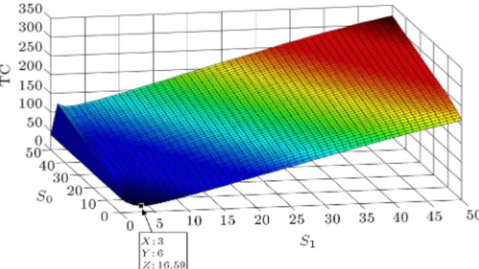
Appendix A
Convexity of Eq. (19)
To investigate the convexity of the approximated total cost function in Eq. (19), we consider a basic case with the following parameters:
c = 5; h0= 2; h1= 1;
0= 1= 0:3; 1= 2;
m = 2; p = 5; and = 20:
For this example, a 3-dimensional graph of TC(S0; S1)
(Eq. (19)) as a function of the two variables S0and S1
is provided using Matlab Software. As can be seen in Figure A.1, TC(S0; S1) is not convex.
Figure A.1. The graph of TC(S0; S1) for the basic
(S1+ 1)
(S1) =
e 1(10+m)(1+ m)S1
e 1010 1S1+1
(S1+1)! + R0
1+m
0 1
xS1e 1x
S1! dx
S1!
e 1(10+m)(10+ m)S1 1
e 1010 1S1
S1! + R0
1+m
0 1
xS1 1e 1x
(S1 1)! dx
(S1 1)!
=(
0 1+ m)
n
(e 11010S1=S1) +R 0 1+m
0 1 x
S1 1e 1xdxo
e 11010S1+1=(S1+ 1)
+R10+m
0 1 x
S1e 1xdx
> (
0 1+ m)
n
(e 11010S1=S1) +R 0 1+m
0 1 x
S1 1e 1xdx o
e 11010S1+1=(S1+ 1)
+ (0 1+ m)
R0 1+m
0 1 x
S1 1e 1xdx
=(e
1100
1S1+1=S1) + (me 1100
1S1=S1) + (10 + m)
R0 1+m
0 1 x
S1 1e 1xdx
e 11010S1+1=(S1+ 1)
+ (0 1+ m)
R0 1+m
0 1 x
S1 1e 1xdx
> 1:
Box I
(S1) = e
1(10+m)(0
1+ m)S1 1
e 1010 1S1
S1! + R0
1+m
0 1
xS1 1e 1x
(S1 1)! dx
(S1 1)!
= e 1(
0 1+m)
e 010 1S1
S1(10+m)S1 1 + R0
1+m 0 1 x 0 1+m S1 1
e 1xdx
> e 1(
0 1+m)
e 010 1S1
S1(10+m)S1 1 + R0
1+m 0 1 x 0 1+m S1 1
dx =
e 1(10+m)
e 1010 1 S1 0 0 1+m
S1 1
+ (10+m)S1
S1(10+m)S1 1
0 1S1
S1(10+m)S1 1
= S1e 1(
0 1+m) e 11010
0
0 1+m
S1 1 + 0
1+ m 10
0
0 1+m
S1 1:
Box II
Appendix B Proof of Lemma 1
First, we show that (S1) is increasing in S1, which
is same as showing that (S1+1)
(S1) > 1. From Eqs. (4)
and (5), the equation shown in Box I is obtained. Furthermore, for the second part, the equation shown in Box II is obtained, where:
lim
S1!1
S1e 1(10+m)
e 11010
0 1 0 1+m +0
1+m 10
0
0 1+m
S1 1=1:
Biographies
Anwar Mahmoodi is currently a PhD candidate in Industrial Engineering at Sharif University of Technol-ogy. He received his BSc in Industrial Engineering from
Isfahan University of Technology and his MSc degree from Sharif University of Technology. His research interests include supply chain management, inventory control, and queuing theory.
Alireza Haji is currently an Associate Professor of Industrial Engineering at Sharif University of Tech-nology, Tehran, Iran. He received his BSc, MSc, and PhD degrees in Industrial Engineering from Sharif University of Technology, Tehran, Iran, in 1987, 1991, and 2001, respectively. His research interests include inventory control, project control, project manage-ment, stochastic models, and queuing systems. Rasoul Haji is currently a Professor of Industrial Engineering at Sharif University of Technology in Tehran, Iran. He received a BSc degree from University
of Tehran in Chemical Engineering, in 1964. In 1967, he received his MSc degree and then, in 1970, his PhD degree both in Industrial Engineering from the University of California-Berkeley. He is recognized as
a co-founder of a fundamental and important relation in queuing theory, known as \Distributional Little's Law". His research interests include inventory control, stochastic processes, and queuing theory.