A Meshless Boundary Element Method
Formulation for Transient Heat
Conduction Problems with Heat Sources
M.R. Hematiyan
and G. Karami
1In the boundary element formulation of heat conduction, the heat source eect imposes an additional domain integral term on the system of integral equations. With this term, an important advantage of the boundary element method as a boundary-only formulation will be lost. This paper presents an accurate method for the evaluation of heat source domain integrals, with no need of domain discretization. Transformation of the domain integral into the corresponding boundary integral is carried out using Green's theorem. Both time-dependent and time-independent fundamental solutions are considered. The methodology can be implemented in general and for similar situations. Numerical examples will be presented to demonstrate the accuracy and eciency of the presented method.
INTRODUCTION
The Boundary Element Method (BEM) is an ecient and accurate numerical technique for heat conduction analysis. The BEM formulation of heat conduction includes several boundary and domain integrals. One domain integral is associated with time rate formula-tion in the form of initial condiformula-tions, and the other one includes the contribution due to heat sources. The direct numerical evaluation of domain integrals neces-sitates the discretization of the domain into internal elements. Although domain discretization does not in-troduce additional unknowns to the nal equations, an important advantage of the boundary element method as a boundary only formulation will disappear. Hence, a method is required to transform the domain integral to the boundary. For the transformation of such integrals in BEM, several schemes have been proposed. For a steady state analysis of the heat conduction problem, the Dual Reciprocity Method (DRM) and the Multiple Reciprocity Method (MRM) were presented by Nardini & Brebbia [1] and Nowak & Brebbia [2,3],
*. Corresponding Author, Department of Mechanical Engi-neering, School of EngiEngi-neering, Shiraz University, Shi-raz, I.R. Iran. E-mail: [email protected]
1. Department of Mechanical Engineering and Applied Me-chanics, North Dakota State University, Fargo, ND 58104, USA.
respectively. In addition, Tang et al. [4] used the Fourier series to represent particular solutions in order to transform integrals to the boundary.
For the transient analysis of heat conduction problems, two classes of formulation have been con-sidered. In the rst class [5-9], a time-dependent fundamental solution is used, and in the second class (including DRM [10] and MRM [11], particular in-tegrals [12] and the radial integration method [13]), a time-independent fundamental solution is used. In DRM [10], the domain terms are approximated by a series of localized particular solutions. This approxima-tion permits the domain integral to be converted into boundary integrals by a simple integration by parts. In MRM [11], high order fundamental solutions are used. Although DRM and MRM are computationally cost eective for transient analysis, they do not include the advantages of the time dependent fundamental solution. In particular, when time steps are selected to be small, DRM and MRM show unstable behavior. Yang et. al [12] employed the particular integrals method for the transformation domain integrals of a heat conduction problem to boundary integrals. Gao [13] used the radial integration method (RIM) for the transformation of domain integrals into boundary integrals. In RIM, the integrand of the domain integral is expressed in a radial form. The domain integral is, then converted to a one-dimensional integral and a boundary integral.
In other elds of analysis, the transformation of the domain integrals has played an ecient role. In elasticity, researchers have introduced several schemes for transforming the domain integrals. Among these schemes is the Galerkin tensor method, which was introduced by Cruse [14] and which was applied to a limited range of body force problems. Danson [15] has also presented a unied treatment for the trans-formation of body force domain integrals into surface integrals, using the concept of the Galerkin vector. Rizzo and Shippy [16] and Karami and Kuhn [17] presented an ecient method based on replacing body force and temperature changes by a scalar potential function. Dual reciprocity and multiple reciprocity techniques were presented by Nardini and Brebbia [18] and Neves and Brebbia [19]. A particular integral concept in boundary element modeling, in conjunc-tion with employing a global shape funcconjunc-tion for the temperature distribution, was presented by Henry & Banerjee [20]. Other solutions include the exact transformation of anisotropic domain integrals (see for example [21]).
In this paper, by using Green's lemma, the domain integrals associated with non-uniform heat sources are transformed to the boundary. The method to be presented here is general enough to be used by employing both either dependent or time-independent fundamental solutions. The method is also successful in solving problems with multiple con-nected regions and can be extended to other two dimensional problems with arbitrary domain loading or non-uniform body forces.
It is clear that the method to be presented here is more complex, from a mathematical point of view, than conventional BEM. However, because of the meshless nature of the present approach, the method will be much simpler from a user's point of view.
THE BOUNDARY INTEGRAL EQUATION OF TRANSIENT HEAT CONDUCTION The governing equation of transient heat conduction with constant material parameters is expressed as follows:
r2T (X; t) + 1
kg(X; t) = 1
@
@tT (X; t); (1)
where T (X; t) is the temperature at point X at time t. The thermal diusivity, , is equal to k
c, in terms
of conductivity, k, density, and specic heat, c, respectively. g(X; t) is the heat source function and is considered to be a function of position and time. The boundary integral form of Equation 1, for a problem with domain and boundary , can be expressed as
follows [5]:
C(P )T (P; tf) +
Z Z tf
t0
T (Q; )q(P; t
f; Q; )dd
= Z Z tf
t0
T (Q; )T(P; t
f; Q; )dd
+k Z
Z tf
t0
g(Q; )T(P; t
f; Q; )dd
+ Z
T (Q; t0)T (P; t
f; Q; t0)d; (2)
where P and Q are, respectively, source and eld points within the domain or on the boundary and C(P ) is a coecient, related to the local geometry at point P . The initial and nal time are represented by t0 and tf, respectively. T is the time dependent
fundamental solution for the diusion equation, which has the following form [22]:
T(P; t; Q; ) = 1
4(t )exp
r2
4(t )
H(t ); where H is the Heaviside function. In the above equation, r is the Euclidian distance between P and Q. The normal derivative of the fundamental solution is denoted by q, where:
q(P; t; Q; ) = @
@nT(P; t; Q; ) = 82(t )r 2exp
r2
4(t )
H(t )@n@r: There are two domain integrals in Equation 2, which include the contribution, due to the heat source and ini-tial conditions. If one assumes that the domain integral associated with the initial condition vanishes (i.e., the initial temperature eld is constant or stationary [7]), by assuming t0 = 0 and tf = tn+1 (tn: current time,
tn+1: new time), one may obtain the following:
C(P )T (P; tn+1) +
Z Z tn+1
tn
T (Q; )q(P; t
n+1; Q; )dd
=
Z Z tn+1
tn
q(Q; )T(P; t
n+1; Q; )dd
+k Z
Z tn+1
0 g(Q; )T
(P; t
n+1; Q; )dd
+ Z Z tn
0 [q(Q; )T (P; t
n+1; Q; )
T (Q; )q(P; t
In the above equation, the only domain integral is the third integral that is as follows:
Ign+1 =
k Z
Z tn+1
0 g[Q(x1; x2); ]
T[P; t
n+1; Q(x1; x2); ]dd; (4)
where (x1; x2) indicate the coordinates of the eld
point. For a direct numerical evaluation of the domain integral (Equation 4), the domain under consideration should be discretized. In such a case, the important advantage of the boundary element method as a bound-ary solution technique would be considerably lost. In this paper, an attempt is made to transfer the domain integral, Ign+1, to the boundary, in order to derive a
boundary-only formulation.
EVALUATION OF THE HEAT SOURCE INTEGRAL
In this section, an accurate and relatively ecient method to evaluate the heat source domain integral is presented. To do so, Green's theorem is used, which relates the domain integral of a two-dimensional region to the boundary. Green's theorem is expressed as follows [23]:
Z
@
@x1R(x1; x2)d =
Z
R(x1; x2)dx2:
This relation can be applied to simply or multiply connected regions, provided that the function, S, is continuous at all points on and on the boundary, . By setting R(x1; x2) as follows:
R(x1; x2) =k
Z x1
a
Z tn+1
0 g[Q(x
0; x 2); ]
T[P; t
n+1; Q(x0; x2); ]ddx;0 (5)
the following relation is obtained: Ign+1 =
k
Z Z x1
a
Z tn+1
0 g[Q(x
0; x 2); ]
T[P; t
n+1; Q(x0; x2); ]ddx0dx2: (6)
The constant a in Equations 5 and 6 is an arbitrary constant. As a suitable value for a, one can set the following:
a =x1 min+ x1 max
2 ;
where x1 minand x1 maxare, respectively, the minimum
and maximum values of the rst coordinate of the boundary points.
As can be seen, the time integral in Equation 6 must be calculated from zero to tn+1, the fact of which
causes too much computation, which, subsequently, becomes ineective and expensive. To overcome this diculty, one can use the fact that the fundamental solution decays with time and, therefore, one can eliminate several initial time steps. The same pro-cedure can also be used to evaluate the last integral in Equation 3 [24]. In the present study, for better accuracy, all time steps are considered for evaluation of the time integral. For cases where the heat generation function is time independent, this diculty can be eectively eliminated. In this respect, one can write as follows:
Ign+1 Ign=
k
Z Z x1
a
Z tn+1
0 g[Q(x
0; x 2)]
exph r2(x0;x2)
4(tn+1 )
i
4(tn+1 ) ddx
0dx 2
k
Z Z x1
a
Z tn
0 g[Q(x 0; x
2)]
exph r2(x0;x2)
4(tn )
i
4(tn ) ddx
0dx
2: (7)
By introducing a new variable, w = tn+1 , for the
rst integral and w = tn for the second integral in
Equation 7, one can write the following: Ign+1 Ign=
1 4k
Z Z x1
a
Z 0
tn+1
g[Q(x0; x 2)]
exph r2(x0;x2)
4w
i
w dwdx0dx2 +4k1
Z Z x1
a
Z 0 tn
g[Q(x0; x 2)]
exph r2(x0;x2)
4w
i
w dwdx0dx2; or:
Ign+1 = Ign+
1 4k
Z Z x1
a
Z tn+1
tn
g[Q(x0; x 2)]
exph r2(x0;x2)
4w
i
w dwdx0dx2:
can be computed by integration at only one time interval.
NUMERICAL IMPLEMENTATION
As T and q vary considerably more slowly than T
and q, one can assume that they are constant over a
small interval of time, (t = tn+1 tn). Hence, q and
T may be taken out of the time integration. By this formulation, only the geometrical boundary must be discretized. If boundary is discretized into N linear boundary elements, the integral Equation 3, may be written as:
C(Pi)T (Pi; tn+1) + N
X
j=1
Z
j
T (Qj; tn+1)
Z tn+1
tn
q(P
i; tn+1; Qj; )dd j = N
X
j=1
Z
j
q(Qj; tn+1)
Z tn+1
tn
T(P
i; tn+1; Qj; )dd + n X m=1 N X j=1 Z j "
q(Qj; tm)
Z tm
tm 1
T(P
i; tn+1; Qj; )d T (Qj; tm)
Z tm
tm 1
q(P
i; tn+1; Qj; )d
#
d j+k n+1 X m=1 N X j=1 Z j
Z x1
a
Z tm
tm 1
g[Q(x0; x
2); ]T(Pi; tn+1; Qj; )ddx0dx2: (8)
Subscript i is an index to represent the node number on the boundary.
The time integrals containing T and q can be
evaluated, analytically as follows: gij=
Z tn+1
tn
T(P
i; tn+1; Qj; )d =41 Ei
r2
4t
; hij=
Z tn+1
tn
q(P
i; tn+1; Qj; )d=2r1 exp
r2 4t @r @n; gm ij =
Z tm
tm 1
T(P
i; tn+1; Qj; )d
= 1 4 " Ei r2
4(tn+1 tm 1)
Ei
r2
4(tn+1 tm)
# ;
hm ij =
Z tm
tm 1
q(P
i; tn+1; Qj; )d
= 2r1 "
exp
r2
4(tn+1 tm 1)
exp
r2
4(tn+1 tm)
# @r @n;
where Ei() is the exponential integral function, i.e. as follows: Ei(a) = Z 1 a exp( x) x dx:
The last time integral in Equation 8 cannot be eval-uated by analytical means. To evaluate this integral, numerically, constant elements over time are used, i.e. g and T are set to be constant over tm 1 < < tm
and are evaluated at midpoint ( = tm 0:5t).
Consequently, Equation 6 takes the following form: C(Pi)T (Pi; tn+1) +
N
X
j=1
Z
j
hijT (Qj; tn+1)d j
=XN
j=1
Z
j
gijq(Qj; tn+1)d j
+ n X m=1 N X j=1 Z j gm
ijq(Qj; tm) hmijT (Qj; tm)d j
+tk n+1X
m=1 N X j=1 Z j
Z x1
a g[Q(x 0; x
2); tm
0:5t]T(P
i; tn+1; Qj; tm 0:5t)dx0dx2: (9)
Regular boundary integrals in Equation 9 are evaluated by a standard 6-point Gauss quadrature method. Since the integrand of the inner integral in Equation 9 may have a severe variation in the integral interval, (a x1), the integral must be evaluated with special
attention. Here, in this research, this integral is evaluated using an adaptive version of the Simpson method. The adaptive Simpson integration method is described in the next section. By adaptive integration methods, one can nd a complicated integral with a desired accuracy.
The evaluation of singular integrals appearing in the formulation is not a dicult task. For this matter, the treatment given in [25] is employed.
Equation 9 can be written in matrix form as follows:
where H and G are coecient matrices, Tn+1 and
qn+1 are temperature and heat ux vectors at time
n+1, respectively, Fn+1 is a vector associated with a
history of the previous steps and Ln+1 represents a
vector associated with heat sources.
For cases where the heat source function is not a function of time, one can write:
Lin+1 = Lin+
t 2k
N
X
j=1
Z
j
Z x1
a g[Q(x 0; x
2)]
exph r2(x0;x2)
2(tn+tn+1)
i (tn+ tn+1) dx
0dx 2:
In writing the above equation, the integral over w = tn
to w = tn+1 is approximated by a constant element,
i.e. the integrand is set to be constant over the time element and is evaluated at midpoint (w = tn+tn+1
2 ).
ADAPTIVE SIMPSON METHOD
Assume that it is desired to compute I = Rabf(x)dx, with tolerance ". This integral can be expressed by Simpson's rule with an interval size, h = (b a)=2 (two intervals, n = 2) as follows:
I = S(a; b) h905f(4)(!); ! 2 [a; b]; (10)
where: S(a; b) = h
3[f(a) + 4f(a + h) + f(b)]: (11) Integral I with four intervals (n = 4) can be expressed by the following relation:
I =S
a;a + b2
+S
a + b 2 ; b
1 16
h5
90
f(4)(!);
! 2 [a; b]: (12)
As an approximation, one assumes f(4)(!)
f(4)(!) [26]. By considering this assumption, one can
show the following: h5
90f(4)(!) 16 15 "
S(a; b) S
a;a + b2
S
a + b 2 ; b
#
: (13)
Now, the error of Simpson's rule, with 4 intervals, can be estimated as follows:
Error =I S
a;a + b2
S
a + b 2 ; b
151 S(a;b) S
a;a+b2
S
a+b
2 ; b
: (14)
If the error computed by Equation 14 is greater than ", the procedure is applied separately to intervalsa;a+b
2
anda+b
2 ; b
, with a tolerance of "
2 for each subinterval.
This halving procedure is continued until each portion is within the required tolerance.
EVALUATION OF THE HEAT SOURCE INTEGRAL IN OTHER FORMULATIONS WITH A TIME INDEPENDENT
FUNDAMENTAL SOLUTION
As mentioned previously in the introduction, in some boundary element formulations of heat conduction analysis, a time-independent fundamental solution is employed [10-13]. In such cases, the heat source integral may be expressed as follows:
Ig= 1k
Z
g(x1; x2)T
[P ; Q(x
1; x2)]d; (15)
where P and Q are, respectively, source and eld points within the domain or on the boundary and T is the
time independent fundamental solution, which has the following form:
T(P ; Q) = 1
2ln
1 r(P ; Q)
;
in which r is the Euclidean distance between P and Q. By applying Green's lemma to Integral 15, the associated boundary integral is obtained as follows:
Ig= 1k
Z Z x1
a g(x 0; x
2)T[P ; Q(x0; x2)]dx0dx2:
For special cases, where heat generation function, g, is to be considered uniformly distributed (g = g0) over
the domain, the integral takes the following form: Ig=2kg0
Z Z x1
aln
1 p
(x0 xs1)2+(x2 xx2)2
! dx0dx
2;
where (xs1; xs2) are coordinates of the source point.
In this case, the inner integral can be evaluated, analytically. For a = 0, it can be expressed as follows:
Ig= 2kg0
Z
[(x1 xs1) ln r
+ (x2 xs2) tan 1
x1 xs1
x2 xs2
(x1 xs1)]dx2:
(16) When the boundary, , is discretized by linear ele-ments, the boundary integral (Equation 16) can also be computed analytically. This would enhance the accuracy of the solutions, especially when the body is thin or the geometric boundary of the domain is complex.
If one assumes Igj to be the heat source integral
over a linear boundary element, j, with starting and
ending points, P1(x11; x12) and P2(x21; x22), then Igj
can be written as follows: Igj = g0(x2k22 x12)
1
Z
0
h
(x1 xs1) ln r
+ (x2 xs2) tan 1
x1 xs1
x2 xs2
(x1 xs1)
i d; where is a local coordinate associated with the element and:
x1= x11(1 ) + x21; x2= x12(1 ) + x22;
r = p
[x11(1 )+x21 xs1]2+[x12(1 )+x22 xs2]2:
(17) Now, one can write as follows:
Igj = g0(x2k22 x12)(Igj1+ Igj2+ Igj3):
The integrals, Igj1, Igj2 and Igj3 are evaluated as
follows: Igj1=
1
Z
0
(x1 xs1) ln rd
=
1
Z
0
(a1+ b1) ln
p
c12+ d1 + e1d; (18)
where:
a1= x11 xs1; b1= x21 x11; c1= rP21P2;
d1= r2sP2 r2P1P2 r2sP1; e1= rsP2 1:
rsP1 and rsP2are Euclidian distances from source point
to P1 and P2, respectively, and rP1P2 is the length of
the element. The analytical evaluation of Integral 18 is described in the Appendix.
The second integral, Igj2, is expressed as follows:
Igj2=
1
Z
0
(x2 xs2) tan 1
x1 xs1
x2 xs2
d:
By substituting x1 and x2 from Equations 17 to the
above integral, it takes the following form: Igj2=
1
Z
0
(a2+ b2) tan 1
c2 + d2
e2 + f2
d; (19)
where:
a2= x12 xs2; b2= x22 x12;
c2= x21 x11; d2= x11 xs1;
e2= x22 x12; f2= x12 xs2:
An analytical evaluation of Integral 19 is given in the Appendix.
The integral, Igj3, is expressed as follows:
Igj3=
1
Z
0
(x1 xs1)d = xs1 12(x21+ x11);
when the source point coincides with any nodes of the element, Igj can be expressed as follows:
Igj= g0(x122kx22)nx21 8 x11
ln rP1P2
1 2
+12(x22 x12) tan 1
x21 x11
x22 x12
1
2(x21 x11) o
: In the above equation, = +1, when the source point coincides with node P1, and = 1, when the source
point coincides with node P2.
EXAMPLES
Three dierent examples are presented to show the accuracy of the proposed method. Two examples are concerned with a transient analysis with a time-dependent fundamental solution and the third example is focused on an analysis with a time-independent fundamental solution. The results are compared with those of analytical or Finite Element Method (FEM) solutions. Whenever FEM is employed, the domain of the problem is discretized by a large number of ele-ments (ne mesh) and the Crank-Nicolson scheme [27] is used.
Example 1: Non-Uniform Time-Independent Heat Source
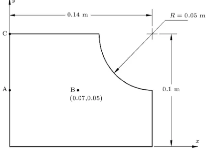
The domain shown in Figure 1 is considered to be subjected to a time-independent heat source, with a distribution of g(x; y) = 106(1 + sin 40x + 10y).
The initial temperature eld is equal to 0.0C and
the boundary condition is of a Robin type, with an ambient temperature of 0.0C and a heat transfer
coecient of 200 W
m2C. Thermal conductivity and
thermal diusivity are set to be k = 80:2 W mC and
= 2:28 10 5 m2
s , respectively.
Results for the temperature variation, with re-spect to time, are presented at three dierent points,
Figure 1. The geometrical domain of the problem.
A, B and C. Points A, B and C are, respectively, a boundary point, an internal point and a corner point. The obtained results are compared with the FEM solution.
For FEM analysis, the domain of the problem is discretized by 512 quadrilateral elements and 559 nodes (Figure 2). For BEM analysis, the boundary of the problem is discretized by 46 linear elements (Figure 3). Figures 4 to 6 compare the FEM solution (t = 10 sec) with results of the present work (t = 20 sec) at the three points, A, B and C. As can be seen, there is a small dierence between the solutions of the BEM analysis and FEM. In problems with a strong variation in heat source function, the FEM can produce an acceptable solution, only with a large number of elements, whereas the solutions obtained by BEM will be acceptable, even with a moderate number of boundary elements.
Example 2: Non-Uniform Time-Dependent Heat Source
In this example, the geometry of the problem, the ini-tial conditions and material properties are considered
Figure 2. FEM discretization of the domain.
to be identical to the previous example. The only dierence is the form of heat generation function, which is assumed to be as follows:
g(x; y) = 106(1 + sin 40x + 10y)f(t):
Figure 3. BEM discretization of the domain.
Figure 4. Temperature variation at point A, Example 1.
Figure 6. Temperature variation at point C, Example 1.
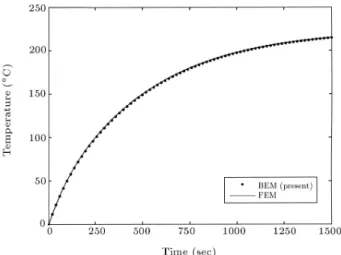
The function, f(t), is chosen to have a variation over time as shown in Figure 7. The results are presented for the temperature at the three points, A, B and C. Figures 8 to 10 compare the FEM solution (512 quadrilateral elements, t = 2:5 sec) with the results of the present work (46 linear boundary elements, t = 5 sec) at the three points, A, B and C. The temperature variations along the lower edge at two dierent times (t = 50 sec, t = 100 sec), are also shown in Figure 11. As seen, the obtained results by the proposed method are in good agreement with the accurate nite element solution.
Example 3: Uniform Heat Source with Time Independent Fundamental Solution
In the two previous examples, the temperature dis-tribution was studied through a simply connected domain, whereas in the example under consideration here, the steady temperature will be studied within a multiply connected domain.
Figure 7. Variation of f(t) with respect to time.
A hollow cylinder, with internal and external radii of ri and ro, is subjected to a uniform heat source with
intensity g0. The boundary surfaces at r = ri and
r = roare kept at temperatures Tiand To, respectively.
Figure 8. Temperature variation at point A, Example 2.
Figure 9. Temperature variation at point B, Example 2.
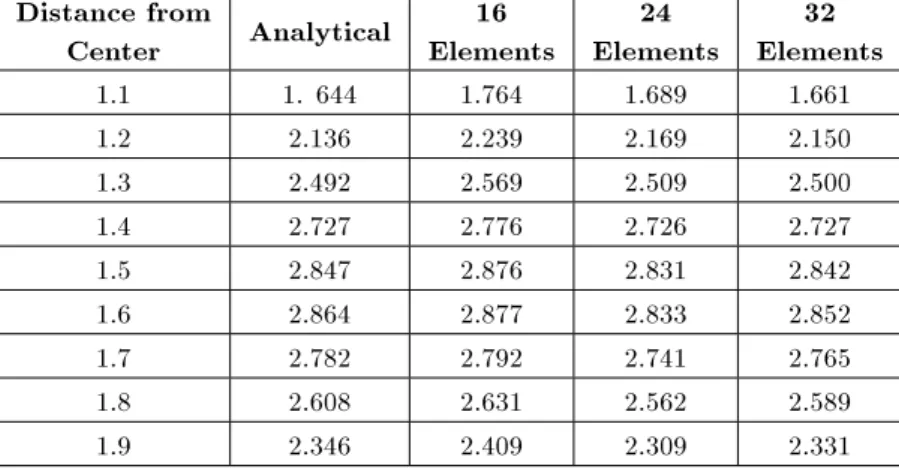
Table 1. Results of analytical and boundary element solutions. Distance from
Center Analytical
16 Elements
24 Elements
32 Elements 1.1 1. 644 1.764 1.689 1.661 1.2 2.136 2.239 2.169 2.150 1.3 2.492 2.569 2.509 2.500 1.4 2.727 2.776 2.726 2.727 1.5 2.847 2.876 2.831 2.842 1.6 2.864 2.877 2.833 2.852 1.7 2.782 2.792 2.741 2.765 1.8 2.608 2.631 2.562 2.589 1.9 2.346 2.409 2.309 2.331
Figure 11. Temperature variation along the lower edge, Example 2.
The governing equation of this problem has the following form:
1 r
d dr
rdTdr
+gk0 = 0:
This has an exact solution as follows: T = 4kg0r2+ c
1ln r + c2;
where:
c1= [To Ti+ g0
4k(r2o ri2)]
lnro
ri
; c2= Ti+g4k0r2i c1ln ri:
This problem is solved with dierent numbers of boundary elements with Ti= 1C, To= 2C, ri= 1 m,
ro= 2 m, k = 1 mWC and g0 = 10 mW3. For boundary
element analysis, both outer and inner boundaries must
be discretized. Table 1 compares the analytical solution at several points with the numerical results obtained when the boundary of the domain is discretized into 16, 24 and 32 linear boundary elements, respectively. As seen, the obtained results are satisfactory.
CONCLUSION
In this paper, a meshless boundary element method for the analysis of heat conduction problems was presented. The method can be implemented for various kinds of BEM heat conduction formulations, includ-ing time-dependent or time-independent fundamental solutions. Although it cannot be used for three-dimensional problems, it can be eciently employed for the treatment of body-force or domain loading in other related two-dimensional elds of analysis.
For stationary and for transient analysis with time-independent heat sources, the method is pletely cost eective, however, it will introduce a com-putational load for the treatment of time-dependent heat sources. An attractive advantage of the present method is its excellent accuracy, especially for the treatment of domain sources, which have severe varia-tions inside the domain.
In conventional BEM, domain integrals are eval-uated by internal discretization and the accuracy of calculated values for domain integrals is directly depen-dent on the size of internal cells. In the present method, domain integrals are evaluated by a boundary integral and a simple 1-D integral, which is evaluated by an adaptive integration method. By using the adaptive integration method, the integrals can be evaluated with a desired and controllable accuracy.
REFERENCES
1. Nardini, D. and Brebbia, C.A. \The solution of parabolic and hyperbolic problems using an alternative boundary element formulation", in Boundary
Ele-ment Methods in Engineering, Proc. of the VIIth Int. Conference, Computational Mechanics Publications, Southampton and Boston, Sprigner-Verlag, Berlin, (1986).
2. Nowak, A.J. \Temperature elds in domains with heat sources using boundary only formulations", in Boundary Element Method, Proc. of 10th Conference, C.A. Brebbia, Ed., Springer-Verlag, Berlin, 2, pp 233-247 (1988).
3. Nowak, A.J. and Brebbia, C.A. \The multiple reci-procity method - A new approach for transforming BEM domain integrals to the boundary", Engineering Analysis with Boundary Elements, 6(3), pp 164-168 (1989).
4. Tang, W., Brebbia, C.A. and Telles, J.C.F. \A gen-eralized approach to transfer the domain integrals into boundary ones for potential problems in BEM", in Boundary Element Methods in Engineering, Proc. of the IX Int. Conference, Computational Mechanics Publications, Southampton and Boston (1987). 5. Brebbia, C.A., Telles, J.C.F. and Wrobel, L.C.,
Bound-ary Element Techniques: Theory and Applications in Engineering, Springer-Verlag, Berlin (1984).
6. Fernandes, J.L.M. and Pina, H.L.G. \Unsteady heat conduction using the boundary element method", in Boundary Element Methods in Engineering, C.A. Brebbia, Ed., Springer-Verlag, Berlin, pp 156-170 (1982).
7. Pasquetti, R. and Caruso, A. \Boundary element ap-proach for transient and nonlinear thermal diusion", Numer. Heat Transfer, Part B, 17, pp 83-89 (1990). 8. Dargush, G.F. and Banerjee, P.K. \Application of the
boundary element method to transient heat conduc-tion", International Journal for Numerical Methods in Engineering, 31, pp 1231-1244 (1991).
9. Ochiai, Y., Sladek, V. and Sladek, J. \Transient heat conduction analysis by triple-reciprocity boundary el-ement method", Engineering Analysis with Boundary Elements, 30, pp 194-204 (2006).
10. Brebbia, C.A. and Wrobel, L.C. \The dual reciprocity boundary element formulation for non-linear diusion problems", Computer Methods in Applied Mechanics and Engineering, 65, pp 147-164 (1987).
11. Nowak, A.J. \The multiple reciprocity method of solving transient heat conduction problems", in Ad-vances in Boundary Elements, 2, Field and Fluid Flow Solutions, C.A. Brebbia and J.J. Connor, Eds., Cambridge, USA, pp 81-93 (1989).
12. Yang, M.T., Park, K.H. and Banerjee, P.K. \2D and 3D transient heat conduction analysis by BEM via particular integrals", Computer Methods in Applied Mechanics and Engineering, 191, pp 1701-1722 (2002). 13. Gao, X.W. \A meshless BEM for isotropic heat con-duction problems with heat generation and spatially varying conductivity", International Journal for Nu-merical Methods in Engineering, 66, pp 1411-1431 (2006).
14. Cruse, T.A. \Boundary integral equation method for three-dimensional elastic fracture mechanics analysis", AFOSR-TR-75 0813 Report (1975).
15. Danson, D.J. \A boundary element formulation for problems in linear isotropic elasticity with body forces", in Boundary Element Methods, C.A. Brebbia, Ed., Springer-Verlag (1981).
16. Rizzo, F.J. and Shippy, D.J. \An advanced boundary integral equation method for three-dimensional ther-moelasticity", Int. J. Num. Meth. Engng., 11, pp 1753-1768 (1977).
17. Karami, G. and Kuhn, G. \Implementation of ther-moelastic forces in boundary element analysis of elastic contact and fracture mechanics problems", Eng. Anal. with Boundary Elements, 10, pp 313-322 (1992). 18. Nardini, D. and Brebbia, C.A. \A new approach to
free vibration analysis using boundary elements", in Boundary Element Methods, Springer-Verlag, Berlin (1982).
19. Neves, A.C. and Brebbia, C.A. \The multiple reci-procity boundary element method in elasticity: A new approach for transforming domain integrals to the boundary", Int. J. Num. Meth. Engng., 31, pp 709-727 (1991).
20. Henry, D.P. and Banerjee, P.K. \A new boundary element formulation for two- and three-dimensional thermoelasticity using particular integrals", Int. J. Num. Meth. Engng., 26, pp 2061-2077 (1988). 21. Zhang, J.J., Tan, C.L. and Afagh, F.F. \Treatment of
body-force volume integrals in BEM by exact trans-formation for 2-D anisotropic elasticity", Int. J. Num. Meth. Engng., 40, pp 89-109 (1997).
22. Carslaw, H.S. and Jaeger, J.C., Conduction of Heat in Solids, 2nd Ed., Clarendon Press, Oxford (1959). 23. Wylie, C.R. and Barrett, L.C., Advanced Engineering
Mathematics, 5th Ed., McGraw-Hill (1982).
24. Demirel, V. and Wang, S. \An ecient boundary element method for two-dimensional transient wave propagation problems", Appl. Math Modeling, 11, pp 411-416 (1987).
25. Aliabadi, M.H., The Boundary Element Method, 2, John Wiley & Sons (2002).
26. Burden, R.L. and Faires, J.D., Numerical Analysis, PWS-KENT Publishing Company, 5th Edition (1993). 27. Reddy, J.N., An Introduction to the Finite Element
Method, 2nd Ed., McGraw-Hill (1993).
APPENDIX
Analytical Evaluation of Integrals Igj1 and Igj2
Igj1 and Igj2 are expressed in terms of two other
integrals, I1 and I2. I1is introduced as follows:
I1(a; b; c; d; e) = 1
Z
0
a + b c2+ d + ed;
when d2 4ce = 0, one can write:
I1(a; b; c; d; e) = ac 1 Z 0 + b a + d 2c 2d = a c 2 4 1 Z 0 1 + d 2c d + d 2c b a Z1 0 1 + d 2c d 3 5
= ac "
ln
+ 2cd + d 2c b a 1 + d 2c # =1 =0 ; and, when d2 4ce < 0, one has the following:
I1(a; b; c; d; e) = 2ca 1
Z
0
2 + 2b a
2+d c +ec
d = a 2c 2 4 1 Z 0
2 + d c
2+d c +ec
d +
1
Z
0
2b a dc
2+d c +ec
d 3 5
= 2ca "
ln
2+d
c + e c =1 =0 + 2b a d c Z1 0 1 + d 2c 2 + e c d 2 4c2 d #
= 2ca "
ln
2+d
c + e c + 2b a d c 1 q e c d 2 4c2
tan 1q +2cd e c d 2 4c2 # =1 =0 : I2 is introduced as follows:
I2(a; b; c; d; e; f) = 1
Z
0
a2+ b + c
d2+ e + fd:
By integration by part, one obtains the following: I2(a; b; c; d; e; f) = ad
=1 =0 + 1 Z 0 b ae d
+c afd
d2+ e + f d
= a d+ I1
b ae
d; c af
d ; d; e; f
: Now, Igj1 can be evaluated as follows:
Igj1 =
1
Z
0
(a1+ b1) ln
p
c12+ d1 + e1d:
One can write Igj1= Igj0 1+ Igj001, where:
I0 gj1 = a1
1
Z
0
lnpc12+ d1 + e1d
= a1 ln
p
c12+ d1 + e1
=1 =0 a1 1 Z 0
(2c1 + d1)
2(c12+ d1 + e1)d
= a1 ln
p
c12+ d1 + e1
=1 =0 a1
2I2(2c1; d1; 0; c1; d1; e1): and:
I00 gj1 = b1
1
Z
0
lnpc12+ d1 + e1d
= b212lnpc
12+ d1 + e1
=1 =0 b1 4 1 Z 0
2(2c1 + d1)
(c12+ d1 + e1)d
= b212lnpc
12+ d1 + e1
=1 =0 b1 4 1 Z 0 2
42 c1
d1 + d2 1
c1 2e1
+d1e1
c1
(c12+ d1 + e1)
3 5 d =
" b1
22ln p
c12+ d1 + e1 b412+b4c1d1 1
b1
4I1
d2 1
c1 2e1;
d1e1
c1 ; c1; d1; e1
# =1 =0 : Another integral, which was introduced previously, is Igj2, which is expressed as follows:
Igj2=
1
Z
0
(a2 + b2) tan 1
c2 + d2
e2 + f2
d:
By applying integration by part, one obtains the following:
Igj2=
a22
2 + b2
tan 1c2 + d2
e2 + f2
=1 =0
(c2f2 e2d2) 1
Z
0 a2
22+ b2
(e2
2+ c22)2+ 2(e2f2+ c2d2) + (f22+ d22)d:
When 0 < f2
e2 < 1, one would confront a singularity
(denominator in argument of tan 1 becomes zero at
= f2
e2), which might be easily removed and, thus
the solution to Igj2 becomes as follows:
Igj2=
a2
2 + b2
tan 1c2+ d2
e2+ f2
+ (c2f2 e2d2)I2a22; b2; 0; e22+ c22; 2e2f2
+ 2c2d2; f22+ d22
; where:
=
a22
2 + b2
tan 1c2 + d2
e2 + f2
= f2e2+ = f2e2
for 0 < fe2