Recent multivariate changes in the North Atlantic climate system, with a focus on 2005–2016

R E V I E W

Recent multivariate changes in the North Atlantic climate system,

with a focus on 2005

–

2016

Jon Robson

| Rowan T. Sutton

| Alex Archibald

| Fenwick Cooper

| Matthew Christensen

|

Lesley J. Gray

| N. Penny Holliday

| Claire Macintosh

| Malcolm McMillan

| Ben Moat

|

Maria Russo

| Rachel Tilling

| Ken Carslaw

| Damien Desbruyères

| Owen Embury

|

Daniel L. Feltham

| Daniel P. Grosvenor

| Simon Josey

| Brian King

| Alastair Lewis

|

Gerard D. McCarthy

| Chris Merchant

| Adrian L. New

| Christopher H. O'Reilly

|

Scott M. Osprey

| Katie Read

| Adam Scaife

| Andrew Shepherd

| Bablu Sinha

|

David Smeed

| Doug Smith

| Andrew Ridout

| Tim Woollings

| Mingxi Yang

1_{National Centre for Atmospheric Science, Department of Meteorology, University of Reading, Reading, UK} 2_{National Centre for Atmospheric Science, Department of Chemistry, University of Cambridge, Cambridge, UK} 3_{Atmosphere, Ocean and Planetary Physics, University of Oxford, Oxford, UK}

4_{STFC Rutherford Appleton Laboratory, Oxford, UK} 5

National Oceanography Centre, Southampton, UK

6_{National Centre for Earth Observation, Department of Meteorology, University of Reading, Reading, UK} 7_{Centre for Polar Observations and Modelling, University of Leeds, Leeds, UK}

8_{National Centre for Atmospheric Science, School of Earth and Environment, University of Leeds, Leeds, UK} 9_{IFREMER, Laboratoire d'Océanographie Physique et Spatiale, Plouzané, France}

10_{Centre for Polar Observations and Modelling, Department of Meteorology, University of Reading, Reading, UK} 11_{National Centre for Atmospheric Science, University of York, York, UK}

12_{Irish Climate Analysis and Research UnitS (ICARUS), Department of Geography, National University of Ireland Maynooth, Maynooth, Ireland} 13_{Met Office Hadley Centre, Exeter, UK}

14_{College of Engineering, Maths and Physical Science, University of Exeter, Exeter, UK} 15_{Centre for Polar Observations and Modelling, University College London, London, UK} 16_{Plymouth Marine Laboratory, Plymouth, UK}

Correspondence

Jon Robson, National Centre for Atmospheric Science, Department of Meteorology, University of Reading, Reading, UK.

Email: [email protected]

Funding information

Natural Environment Research Council, Grant/ Award Number: North Atlantic Climate System: Integrated Study (ACSIS)

Major changes are occurring across the North Atlantic climate system, including in the atmosphere, ocean and cryosphere, and many observed changes are unprece-dented in instrumental records. As the changes in the North Atlantic directly affect the climate and air quality of the surrounding continents, it is important to fully understand how and why the changes are taking place, not least to predict how the region will change in the future. To this end, this article characterizes the recent observed changes in the North Atlantic region, especially in the period 2005–2016, across many different aspects of the system including: atmospheric circulation; atmospheric composition; clouds and aerosols; ocean circulation and properties; and the cryosphere. Recent changes include: an increase in the speed of the North Atlantic jet stream in winter; a southward shift in the North Atlantic jet stream in summer, associated with a weakening summer North Atlantic Oscillation; increases

DOI: 10.1002/joc.5815

This is an open access article under the terms of the Creative Commons Attribution License, which permits use, distribution and reproduction in any medium, provided the original work is properly cited.

© 2018 The Authors. International Journal of Climatology published by John Wiley & Sons Ltd on behalf of the Royal Meteorological Society.

in ozone and methane; increases in net absorbed radiation in the mid-latitude west-ern Atlantic, linked to an increase in the abundance of high level clouds and a reduction in low level clouds; cooling of sea surface temperatures in the North Atlantic subpolar gyre, concomitant with increases in the western subtropical gyre, and a decline in the Atlantic Ocean's overturning circulation; a decline in Atlantic sector Arctic sea ice and rapid melting of the Greenland Ice Sheet. There are many interactions between these changes, but these interactions are poorly understood. This article concludes by highlighting some of the key outstanding questions. K E Y W O R D S

atmosphere, atmospheric composition, cryosphere, observations, ocean, north atlantic

1 | I N T R O D U C T I O N

The North Atlantic region has warmed over the past 100 or so years (Stockeret al.,2013; Chenget al.,2017). However, the North Atlantic has also evolved somewhat differently to the rest of the world's oceans on multidecadal time scales, with periods of faster warming and cooling. This variability, which has become known as Atlantic multidecadal variabil-ity (AMV, Sutton et al., 2017), has been linked to a wide range of impacts including rainfall anomalies over Africa, North America and Europe (Sutton and Hodson, 2005; Knight et al.,2006; Sutton and Dong, 2012); the frequency of Hurricanes (Zhang and Delworth, 2006; Smith et al.,

2010); the rate of Greenland ice-sheet melt (Holland et al.,

2008; Hanna et al., 2013a);sea-level anomalies (McCarthy et al., 2015); fisheries (Hátún et al.,2009) and the strength of the mid-latitude atmospheric jet (Woollings et al.,2015). Therefore, uncertainty in how North Atlantic surface temper-atures might change is a major uncertainty in climate projec-tions, especially for the European sector (Woollings

et al.,2012).

Although multidecadal variability has been observed in the North Atlantic, the mechanisms and processes that con-trol this variability are poorly understood. A leading hypoth-esis is that changes in the strength of the ocean circulation, and particularly the Atlantic meridional overturning circula-tion (AMOC), is an important contributor to the variability in the ocean heat content and sea surface temperature (SST) (Knight, 2005; Ba et al.,2014; Menaryet al.,2015). How-ever, although indirect observations suggest ocean circula-tion has led AMV-related changes in the North Atlantic (McCarthy et al., 2015; Robson et al., 2016; Thornalley

et al.,2018), a paucity of observations has prevented a direct link being made between ocean circulation changes and AMV in the real world. There is also a considerable diver-sity in the mechanisms of variability found in climate models and the important feedbacks that control the time scales of variability (Baet al.,2014; Menaryet al.,2015).

Variability in the atmospheric circulation is also an important driver of climate variability across the North Atlantic climate system. The leading mode of atmospheric variability, the North Atlantic Oscillation (NAO), drives inter-annual to multidecadal time-scale variability in vari-ables that span the entire Atlantic climate system, including SST, ocean circulation, troposhperic ozone, surface run off from Greenland and extreme temperatures and rainfall over Europe (Hurrell et al., 2003; Scaife et al., 2008; Pausata

et al., 2012; Robson et al., 2012; Hanna et al., 2014). Indeed, the NAO is often considered a major driver of AMOC, and hence AMV (Eden and Willebrand, 2001; Rob-son et al., 2012; Delworth and Zeng, 2016; Sutton et al.,

2017)—although it has also been hypothesised that the NAO may drive AMV with no need for ocean circulation changes (Clement et al., 2015). On decadal time scales, the NAO may also be influenced by AMV or other changes in North Atlantic conditions such as regional SST anomalies or sea ice changes (Gastineau et al., 2013; Gastineau and Fran-kignoul, 2014; Peings and Magnusdottir, 2014; O'Reilly

et al., 2017; Wang et al., 2017). However, unravelling the interactions between ocean, atmosphere and cryosphere is very challenging, especially in the short observational record.

A further question to consider is the role of external fac-tors in driving changes in the North Atlantic. For example, recent studies have suggested that AMV is a result of com-petition between rising greenhouse gas emissions and regional changes in sulphate aerosols (Booth et al., 2012). Changes in solar irradiance and volcanic aerosols are also thought to be important influences on the atmospheric circu-lation and the NAO, and hence could impact widely across the North Atlantic climate system (Grayet al.,2013; Menary

et al., 2013; Ortega et al., 2015). The long-term warming trend is also changing the climate of the North Atlantic region, especially in the high latitudes, including melting Arctic sea ice and the Greenland Ice sheet (Stocker et al.,

2013) which could influence the oceanic (Swingedouw

circulation. Finally, the presence of global teleconnections, in the atmosphere in particular, means that variability and changes outside the North Atlantic can also have a substan-tial influence (Biastochet al.,2008; Bellet al.,2009).

The composition of the atmosphere in the North Atlantic region has also been changing, and can interact with changes in physical aspects of the climate. Ozone (O3) and methane (CH4) are powerful greenhouse gases and can affect climate by changing the Earth's radiative balance (Stocker et al.,

2013). Tropospheric ozone can also affect human health and agricultural yields (Kampa and Castanas, 2008), and was recently suggested to cause 1.2 million premature deaths per year (Malley et al., 2017). Observed ozone changes are driven by a complex interplay of emission changes in nitro-gen oxides and organic and inorganic radicals, changes in downward transport from the stratosphere, and changes in regional atmospheric circulation affecting transport time scales (see. e.g., Monkset al. (2015) for more details). How-ever, while recent trends in carbon monoxide and methane are generally driven by emission changes (Worden et al.,

2013; Nisbet et al., 2016), the recent observed trends in ozone over the North Atlantic are not fully characterized or understood (Parrishet al.,2014) and require a deeper under-standing of relationships to atmospheric circulation changes.

It follows from the above discussion that there are many important unanswered questions regarding the nature of decadal timescale change in the North Atlantic region, and how changes in different components of the North Atlantic climate system are interlinked. This lack of understanding is a fundamental limit to our ability to understand the current changes, and to our ability to make quantitative predictions of how the North Atlantic climate system will change in the future. However, the large number of important variables and processes involved in the changes, and the complex array of interactions between different components of the North Atlantic climate system, makes understanding the ongoing changes across all components of the North Atlantic climate system extremely challenging. Therefore, there is a need to take a more holistic, and multidisciplinary, view of decadal time-scale variability in the North Atlantic. There-fore, with this end in mind, this article aims to broadly char-acterize and document the observed changes across multiple components of the North Atlantic climate system in one place, and to review of the relevant recent literature. Although the atmosphere has been well observed for many decades, other important variables have not. Therefore, we focus on the observed changes over the recent time period (since 2000) by exploiting the many new observations and improved reanalysis products that have recently become available as a consequence of programmes such as ARGO and RAPID, and satellite products. The period 2006–2015/2016 is a particular focus due to the vastly improved data coverage over all components of the North Atlantic.

This article is structured as follows. Recent changes in atmospheric circulation are described in Section 2, before recent changes in atmospheric composition are discussed in Section 3. Recent changes in aerosols, clouds and radiative effects are described in Section 4, before changes in ocean properties and the cryosphere are discussed in Sections 5 and 6. Finally, a summary and conclusions are presented in Section 7.

2 | R E C E N T C H A N G E S I N A T M O S P H E R I C C I R C U L A T I O N A N D P R O P E R T I E S

In this section, we consider the recent variability and trends in atmospheric circulation over the North Atlantic region. We use data from the European Centre for Medium-Range Weather Forecasts ERA-interim reanalysis (Deeet al.,2011) and, where stated, from the Atmospheric and InfraRed Sounder (AIRS) instrument onboard NASA's Aqua satellite (Tianet al.,2017).

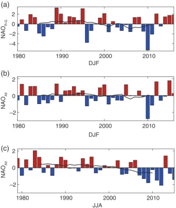
“The North Atlantic Oscillation (NAO) is one of the most prominent and recurrent patterns of atmospheric circu-lation variability”(Hurrellet al.,2003). It is usually defined as the first empirical orthogonal function (EOF) of surface pressure in the region 30W–40E and 20–70N and its time evolution can be illustrated by plotting the correspond-ing principal component time series. An alternative that does not require knowledge of surface pressure over this extended region uses the normalized pressure difference between station-based observations, usually between Azores-Iceland (Hurrell, 1995; Cropperet al.,2015) or between Reykjavík– Gibraltar, (Jones et al., 1997). We employ the Reykjavík– Gibraltar (NAOR-G) index here. The standard EOF-based NAO and the NAOR-Gindicators are very similar in the win-ter season [December–January–February (DJF)], with a cor-relation coefficient of 0.89 over the period 1979–2016.

The recent NAOR-G index averaged over the winter months (DJF) is plotted in Figure 1a. The smoothed 11-year running mean of NAOR-G increases from the mid-1980s, peaks around the early 1990s, and is followed by a down-ward trend (Woollings et al., 2015). The winter of DJF 2009/2010 exhibits a particularly strong negative NAO, although positive values in the more recent years may indi-cate a positive trend. To focus more on how the atmospheric circulation has varied over the North Atlantic Ocean, we also derive an EOF-based index of the NAO (NAOAtl) using the first EOF of surface pressure over the restricted region centred over the Atlantic, that is, 60–0W and 30–70N (Figure 1b; see also Figure S1a, Supporting Information). In comparison with NAOR-G, the 11-year running mean of NAOAtl in DJF is noticeably flatter with respect to its vari-ance, although the correlation of the DJF NAOAtl with NAOR-G is still 0.82. The 11-year running mean of NAOAtl for the summer months (June–July–August; JJA; Figure 1c, with corresponding EOF in Figure S1c) has been on a

continuous downward trend since 1990 and was previously reported as statistically significant (Hanna et al., 2015). (We note from examination of the structure of the first EOF of the JJA surface pressure that the station-based NAOR-Gis not an appropriate indicator of the summer-time circulation [compare A2a and A2b.] and it is therefore not shown).

While the NAO is a useful single indicator of atmo-spheric circulation over the Atlantic and its potential impact on European weather, it is nevertheless a derived quantity combining several factors. Two additional indicators that directly characterize the North Atlantic Jetstream have been proposed: the jet latitude and jet speed (Woollings et al.,

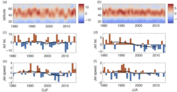
2014). Figure 2a,b shows the DJF and JJA time series of zonal velocity at 850 hPa in the region 60–0W and 15– 75N, to illustrate the spatial evolution of the mid-latitude Jetstream. The jet latitude index (JLI) is defined as the lati-tude of the maximum zonal wind speed at 850 hPa calcu-lated using seasonal mean zonal winds over the region 60– 0W, 15–75N (Figure 2c,d). The JLI is clearly related to NAOAtl (compare Figures 1b,c and 2c,d); positive NAOAtl implies that the jet maximum is somewhat offset to the north. Figure 2c shows that recent trends in the 11-year

running mean of the winter JLI are small in comparison with the interannual variability (Woollings et al., 2014). How-ever, the 1979–2015 southward trend in summer JLI (Figure 2d) is statistically significant at thep< .05% level, consistent with the negative trend in the NAOAtl in JJA (Figure 1c). Note the different scales in Figure 2c,d indicat-ing that variability in winter JLI is larger than in summer.

The jet speed index (Figure 2e,f ) is defined as the maxi-mum zonal velocity in the region 60–0W at the latitude identified by the JLI. It is also more variable in winter than in summer. The 11-year running mean of the winter jet speed peaks in 1990, is a minimum around 2005, and then returns to higher speeds more recently. As the summertime jet has moved southwards in recent years it has also weak-ened (Figure 2f ). Figure 2f also hints that variability in the JJA mean jet speed has reduced.

Comparing the NAO and jet indices, we can see that the negative summer NAO trend over 2005–2016 (Figure 1c) largely reflecting an equatorward jet shift (Figure 2d), with some contribution of a weaker jet (Figure 2f ). In the winter, the trend over 2005–2016 was to a slightly stronger jet (Figure 2e). However, the interannual variability in jet lati-tude (Figure 2c) also made an important contribution to the interannual evolution of the NAO (Figure 1a). An increase in the year-to-year variability of the December NAO (Hanna

et al.,2015) and corresponding jet latitude (Overlandet al.,

2015) has also been reported previously. The equatorward migration of the summertime jet may be linked to AMV (Sutton and Dong, 2012), which transitioned from negative to positive in the mid-1990s (Suttonet al.,2017). Neverthe-less, these changes in the zonal wind speed and latitude have implications for atmospheric heat and water vapour (Deser

et al., 2010) and aerosol (Lewis and Schwartz, 2004) exchange with the Atlantic Ocean, as has been pointed out for the Southern Ocean (Korhonenet al.,2010).

Figure 3 shows trends in the overall seasonal surface pressure fields (rather than only the NAO index). In DJF for both the 1990–2005 and 2006–2016 periods, the pressure trends project strongly onto the second EOF pattern. The dot products of these trends with the second EOF patterns (not shown), both normalized to unit vectors, are 81 and 76%, respectively, while their projection onto the first EOF pattern is weaker (19 and 51%, respectively). In JJA on the other hand, the situation is reversed with stronger projection of trends onto the first EOF (55 and 56%, respectively) than onto the second EOF (17 and 12%, respectively).

In Figure 3, the hatched regions indicate where there is less than a 5% chance (i.e.,p≤.05) that the observed trend is consistent with random variability. We conclude that trends in the seasonal mean surface pressure over the periods considered are small relative to its variance, and the trends will be sensitive to the time periods used. However, over the period 1990–2005, there was a statistically significant increase in pressure over Greenland (also noted by Hanna

1980 1990 2000 2010

–4 –2 0 2

NAO

R-G

DJF

1980 1990 2000 2010

DJF –2

0 2

NAO

Atl

1980 1990 2000 2010

JJA –2

0 2

NAO

Atl

(a)

(b)

(c)

FIGURE 1 (a) NAO index estimated from the normalized difference of surface pressures at Reykjavik and Gibraltar. Each of the surface pressure time series is normalized by their respective standard deviation (SD), so the index is dimensionless. (b) DJF Atlantic NAO index estimated as the surface pressure principal component time series over the region 60–0W, 30–70N. The principal component time series is normalized by itsSD, so the index is dimensionless. (c) JJA Atlantic NAO index otherwise as (b). All plots: The bars indicate the seasonal mean values and the thick black line indicates an 11-year running mean [Colour figure can be viewed at wileyonlinelibrary.com]

et al.,2016). This increase suggests that the 11-year decreas-ing trend in NAO over this period (Figure 1a,b) is potentially associated with a weakening of the Icelandic Low (i.e., the northern node of the NAO). Despite a stronger (positive) trend over 2006–2016 when compared to 1989–2005, the 2006–2016 trend is not significantly different from that expected from random numbers (note also the slightly shorter time period). The summertime pressure trends are smaller than the wintertime trends, but note that this could be due to the smaller variability in summertime.

As an illustration of the vertical distribution of recent circu-lation changes, Figure 4 shows the zonally averaged DJF zonal wind at 60N. Year-to-year changes in the strength of the extratropical westerly jet stream tend to be equivalent barotro-pic and hence vertically aligned throughout the depth of the troposphere and stratosphere. There is also sometimes addi-tional evidence for a downward propagation of zonal wind changes and they show some striking inter-decadal variability. Recent decades have shown substantial variability in the strength of these extratropical winter westerlies. A build-up of strong westerlies occurred from the early 1960s (see, e.g., Figure 3 in Scaife et al. (2005), and also Hanna et al. (2008a) in relation to“storminess”), and is apparent throughout the depth of the atmosphere, eventually peaking in the early 1990s, as evident in Figure 4. These early 1990s winters also coincided with a string of positive episodes of the surface NAO and were accompanied by intense storms, very wet win-ters and a drastic reduction in the number of frost days in

northern Europe (Scaife et al., 2008; Roberts et al., 2014). While the build-up of the westerlies in the early 1990s seen in Figure 4 is related to multidecadal variability rather than a sys-tematic trend, the reasons are still unclear. It is not even known if this is due to forced or internal variability. The proposed explanations involve internal chaotic variability (Semenov

et al., 2008), ocean–atmosphere interaction (Hoerling et al.,

2004; Omraniet al.,2016) and forced responses to volcanism (Marshall and Scaife, 2009; Driscollet al.,2012) or solar vari-ability (Grayet al.,2010; Inesonet al.,2011).

Following the peak winter westerlies in the early 1990s seen in Figure 4, a subsequent decline is evident, with a deep minimum in 2010 that corresponds to the strongly negative NAO in Figure 1a,b. Although the maximum easterly anom-alies are in the troposphere, there is evidence of downward extension from the stratosphere. The 2010 anomaly is also visible as an equatorward shift in the position of the Atlantic westerlies (Figure 2a). The winter of 2009/2010 exhibited the lowest NAO on record (Cattiaux et al., 2010; Seager

et al.,2010; Feredayet al., 2012) and followed in 2010 by the coldest December for a century (Maidens et al., 2013; Blakeret al.,2015). Potential causes of the 2009/2010 weak westerlies includes the extratropical response to El Nino (Fereday et al., 2012), the deep minimum in the 11-year solar cycle (Gray et al., 2013, 2016), the easterly phase of the quasi-biennial oscillation (QBO) (Pascoe et al., 2006; Feredayet al.,2012), and Arctic sea-ice losses (Strong and Magnusdottir, 2011; Wanget al.,2017).

FIGURE 2 Top row: (a) and (b), seasonal and longitudinal average of the zonal velocity as a function of latitude at 850 hPa in the region 60–0W, (m/s). Note the change in colour scale. Middle row: (c) and (d), latitude anomaly (degrees) of the maximum of the seasonal mean zonal velocity at 850 hPa in the region 60–0W, 15–75N. Bottom row: (e) and (f ), anomaly of the maximum of the seasonal mean zonal velocity (m/s) at 850 hPa in the region 60–0W, 15–75N. Left: Index averaged over DJF. Right: Index averaged over JJA. All plots: The bars indicate the monthly mean values and the thick black line indicates an 11-year running mean [Colour figure can be viewed at wileyonlinelibrary.com]

After 2010, the westerlies strengthened again. The recent three winters from 2013/2014 to 2015/2016 were all strong westerly winters with positive surface NAO and numerous win-ter wind storms and abundant rainfall (Huntingfordet al.,2014; Wild et al., 2015; Watson et al.,2016; Scaife et al., 2017).

Recent changes in the Atlantic Ocean surface conditions and tropical rainfall help to explain this recent upturn, which also closely follows the recent solar maximum (Scaifeet al.,2017).

North Atlantic SSTs are strongly influenced by atmo-spheric seasonal variability (see Section 5 of this article and, e.g., Deser et al., 2010). However, surface heat fluxes are governed by a complex function of the wind speed, humidity and temperature differences (e.g., Hewitt et al., 2011, their Figure 1). The 2006–2016 trend in ERA-interim 2 m temper-ature is plotted in Figure 5a,b (DJF, JJA, respectively). The DJF cooling in the North Atlantic region is visible above the background variability, consistent with the 1996–2005 SST trends in Figure 14. The summertime trend (JJA) over this time period is smaller, but shows the same overall pattern of a cooling in the north Atlantic, including over Greenland, and a warming further towards the tropics.

FIGURE 3 Trends in the seasonal mean surface pressure in hPa per decade. Hatched regions are where the trend exceeds the 95% confidence interval for Gaussian distributed random numbers, with one number per season [Colour figure can be viewed at wileyonlinelibrary.com]

FIGURE 4 Seasonal average of the DJF zonal mean zonal wind anomaly at 60N (m/s). The time series on each pressure level has been normalized to have aSDof one in order to highlight the barotropic nature of the flow [Colour figure can be viewed at wileyonlinelibrary.com]

To examine trends at higher levels, the 2006–2016 trends in the seasonal mean 700 hPa air temperature are plot-ted in Figure 5c,d (now as measured by AIRS, to be consis-tent with the water mass mixing ratio plots in Figure 5e,f ).

Although barely distinguishable from the background vari-ability, both the wintertime and summer time 700 hPa trends bear some resemblance to their 2 m equivalents. In DJF, the north Atlantic has cooled at 700 hPa by around 0.15C per

(a) (b)

(c) (d)

(e) (f)

FIGURE 5 Decadal trends over the period 2006–2016. Top row: (a) and (b), 2 m air temperature trend using ERA-interim data. Middle row: (c) and (d), 700 hPa temperature, as measured by AIRS, see http://airs.jpl.nasa.gov. Bottom row: (e) and (f ), 700 hPa water mass mixing ratio, as measured by AIRS [Colour figure can be viewed at wileyonlinelibrary.com]

decade, while warming towards the tropics and the winter-time trend is again much larger than the summerwinter-time. Trends in the 700 hPa water mass mixing ratio (as measured by AIRS) are not distinguishable from the background variabil-ity over this time period. It is not clear how closely the trend patterns for water mass mixing ratio in both DJF and JJA (of around 0.0025 g/kg dry air) reflect the respective 700 hPa temperature trend patterns in the north Atlantic.

3 | R E C E N T C H A N G E S I N A T M O S P H E R I C C O M P O S I T I O N

In this section, we concentrate on tropospheric ozone and methane; two important trace gases for which a recent satel-lite record exists. Ozone is produced in the troposphere through a complex interplay of reactions involving nitrogen oxides and organic and inorganic radicals (see, e.g., Monks

et al. (2015) for more details). Because of its short lifetime in the troposphere (days to weeks), the largest ozone concen-trations are often observed downwind but in close proximity to the sources of precursor gases. Methane, on the other hand, has a much longer lifetime in the troposphere (around 10 years) and is relatively well mixed. Changes in methane concentrations are generally thought to be mainly driven by changes in its emissions, which range from soils in natural wetlands through to fossil fuel production. More recently,

changes in methane concentrations have also been attributed to changes in the concentration of the hydroxyl radical (OH), the main sink for methane, (Schaefer et al., 2016; Prather and Holmes, 2017; Rigbyet al.,2017; Turneret al.,

2017). In this section, we document recent changes using surface observations and monthly mean gridded satellite data. The tropospheric ozone column was calculated from the Ozone Monitoring Instrument (OMI) and Microwave Limb Sounder (MLS) combination (OMI/MLS) as described in Ziemke et al. (2006) while methane total column was derived from the AIRS (Xiong et al., 2008; Yurganov

et al.,2008).

3.1 | Time series of surface ozone at selected monitoring sites, tropospheric ozone column and total methane column

Figure 6 shows recent trends (ca. 2006–2016) of ozone and methane in the North Atlantic as measured at the surface and by satellite. Surface ozone shows a strong seasonal cycle across the North Atlantic, with a peak in spring and a mini-mum in the summer (see Figure 6b). Surface ozone at Ber-muda has been decreasing significantly at a rate of 19.8 ppb/ decade; this is likely due to the significant reduction in emis-sions of ozone precursors in the United States (Granier

et al.,2011). A smaller decrease is observed at Mace Head; in this case, the changes are harder to attribute and may FIGURE 6 Time series from satellite and surface in situ measurements in the North Atlantic. Monthly median surface ozone mixing ratios (panel b) are shown for three long-term monitoring sites in the North Atlantic: Bermuda (64.87E; 32.31N), Cape Verde (24.87E; 16.54N), Mace Head (9.90E; 53.32N) (locations shown on panel a). Satellite trends (panels c and d) are calculated over the period 12/2005–2/2016 (123 months) for average values over three domains: North Atlantic (100W–20E; 0:60N), mid-latitude (100W–20E; 30–60N), subtropical (100W–20E; 0:30N). The curves plotted are 12 months running averages. Tropospheric ozone column trends from monthly OMI-MLS data; methane column trends from AIRS; surface in situ measurements from global atmospheric watch [Colour figure can be viewed at wileyonlinelibrary.com]

reflect local changes to the lifetime of ozone or the effect of large decreases in ozone precursors upwind of Mace Head. In contrast, surface ozone at Cape Verde has been increasing at a rate of 3.6 ppb/decade. This may be related to an increase in shipping, and hence ozone precursor emissions, a decrease in oceanic halogens, an important sink for ozone (Read et al., 2008), or a general effect of the increases in methane, which acts as an important ozone precursor at the global scale (Younget al.,2013).

Changes in tropospheric ozone column, Figure 6c, show a different picture, with a consistent increase across the North Atlantic. Several factors can contribute to trends in background tropospheric ozone including changes in emis-sions of ozone precursors, changes in temperature and solar radiation and long-range transport of ozone and its precur-sors. It has also been suggested that through El Niño/South-ern Oscillation and the stratospheric Quasi-Biennial Oscillation, large-scale changes in climate may be affecting the transport of stratospheric rich ozone into the troposphere (Neuet al.,2014), thereby increasing the tropospheric ozone burden.

The satellite retrievals of total column methane also show a strong, near linear, increase in methane over the North Atlantic in the last decade. This is consistent with our current understanding of global methane trends, for example, (Nisbet et al., 2016). The methane trends are consistent across subregions of the North Atlantic, albeit the total col-umn methane magnitude is smaller in the subtropics than in the mid-latitudes. A lower subtropical methane column is consistent with a shorter lifetime (due to higher concentra-tions of OH), weaker primary sources and stronger mixing into the stratosphere (through deep convection) in the tropics compared to mid-latitudes.

3.2 | Spatial and seasonal variability in observed trends

In this section, we analyse how trends in the observed col-umns of ozone and methane vary spatially and seasonally across the North Atlantic basin. Methane is a relatively long-lived gas which is generally well mixed at a regional scale and therefore very little spatial and seasonal variation in the North Atlantic trends is observed (not shown). On the other hand, ozone shows some interesting spatial variations with generally positive trends ranging between 0 and 15% per decade, depending on location. In winter (top panels of Figure 7), the spatial variability of ozone trends becomes larger with negative ozone trends over the Western part of the North Atlantic domain and very large positive trends over Central Europe and the Eastern part of the North Atlan-tic basin. In summer (middle panels in Figure 7) ozone shows a larger increase in the subtropical North Atlan-tic (STNA).

Observations from a small number of surface stations in the nineteenth century indicate that ozone concentrations

have increased significantly since preindustrial times due to anthropogenic activities (Mickley et al., 2001; Shindell

et al.,2006; Stevensonet al.,2013). In developed countries, a recent reduction in the emissions of ozone precursors (Granieret al., 2011) has helped decrease ozone levels and made an impact at the local and regional scale. However, different observational studies do not provide a consistent picture regarding the sign and magnitude of recent ozone trends at northern mid-latitudes (Cooperet al.,2014; Parrish

et al., 2014; Ebojie et al., 2016; Oetjen et al., 2016). Our FIGURE 7 Decadal linear trends (ca. 2006–2016) calculated using seasonal (DJF [top] and JJA [middle]) and annual-mean (bottom) ozone tropospheric column. Trends are calculated over the period 12/2005–2/2016. The stippling indicates where trends are significant to the 95% confidence level, based on the standard error of the residuals (Wigley et al., 2006). Methane trends show little variation spatially and seasonally (not shown) [Colour figure can be viewed at wileyonlinelibrary.com]

study shows a generally small, but significant, positive trend over the North Atlantic for the period 2006–2016 (Figure 6c and Figure 7). The ozone increase seems to be larger and more robust for the STNA, and also for summer compared to winter. Despite looking at similar quantities, that is, tropo-spheric ozone column, our results and those of Ebojieet al. (2016) and Oetjen et al. (2016) all somewhat differ from each other. This is partly due to significant differences between the observing techniques and the different retrieval schemes applied. Similarly, the differences we identify between observed trends for surface and free tropospheric ozone are likely due to a decoupling between surface ozone (driven by local emission and sinks) and mid-tropospheric ozone (driven by large-scale transport and stratosphere-troposphere exchange (STE)).

3.3 | Impact of NAO on North Atlantic composition and possible effects on observed ozone trends

The positive phase of the NAO can increase the rate of trans-port of ozone and ozone precursors from North America to Europe. Ozone has a relatively short lifetime; therefore, faster transport across the North Atlantic can increase its abundance downwind of source regions. Changes in precipitation patterns (Scaifeet al.,2008) associated with the positive phase of the NAO (wetter than average Northern Europe and drier than average Southern Europe) can additionally affect ozone distri-bution by affecting the concentration of soluble ozone precur-sors. The NAO can also have an impact on modulating strat-trop exchange (Simmonds et al., 2013) which in turn can affect the regional ozone distribution in the North Atlantic.

Several studies have looked at intercontinental transport of tracers and pollutants and the role of the NAO in such transport pathways (Li et al., 2002; Creilson et al., 2003; Pausata et al., 2012). Li et al. (2002) analysed modelled hourly surface ozone at Mace Head, for the period 1993–1997, and found it includes a significant fraction of North American ozone, around 10% on average throughout the year, and rising up to ~30% during transatlantic transport events. Creilson et al. (2003) analysed tropospheric ozone column (from TOMS/SBUV instruments) for the period 1979–2000 and found that, in some regions of the North Atlantic, tropospheric ozone is correlated to the NAO index. Similarly, Pausata et al. (2012) investigated the impact of NAO on ozone and found a positive correlation between the winter NAO index and ozone concentrations from surface stations in the United Kingdom and Northern Europe. They further suggested that summer NAO events could increase ozone concentrations over Europe, at a time when ozone levels are generally highest and could pose a threat to human health. As the NAO exerts a large influence on ozone trans-port over the North Atlantic, understanding future changes in the NAO and its influence on atmospheric composition is an important but little studied task (Baceret al.,2016).

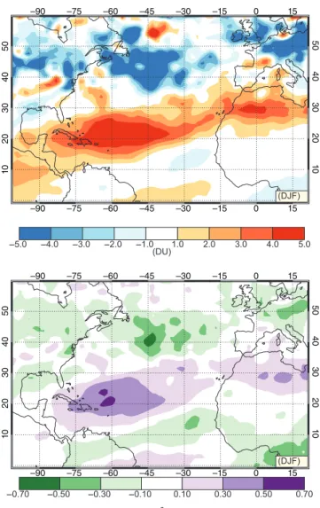
We now focus on whether we can identify any influence of the winter NAO on the tropospheric ozone data used for this study and address whether changes in the NAO could partly explain observed or future ozone trends in the North Atlantic. Figure 8 (top panel) shows the difference in monthly mean tro-pospheric ozone column between winter months with “high” and “low”NAO indices. The top panel of Figure 8 suggests that the tropospheric ozone column decreases by up to 5–6 dob-son units (DU) over large parts of North Europe, the United Kingdom and mid-latitude North Atlantic when the NAO is in its positive phase compared to when it is in its negative phase. Conversely, large areas of North Africa and STNA see an increase in tropospheric ozone column of 5–6 DU when the NAO is in its positive phase. This indicates a sizeable change in tropospheric ozone column over large areas of the North

–90

50

40

30

20

10

50

40

30

20

10

–75 –60 –45 –30 –15 0 15

–90 –75 –60 –45 –30 –15 0 15

–90

50

40

30

20

10

50

40

30

20

10

–75 –60 –45 –30 –15 0 15

–90 –75 –60 –45 –30 –15 0 15

FIGURE 8 Impacts of NAO on tropospheric ozone column. Top panel shows difference in mean ozone tropospheric column between winter months with“high”and“low”NAO indices (high/low are defined as months between 12-2005 and 2-2016 with NAO index greater/smaller than +/−2). Bottom panel shows the correlation coefficient between tropospheric ozone column at each location and winter months NAO indices. NAO index is calculated as the difference between the normalized sea level pressure over Gibraltar and the normalized sea level pressure over SW Iceland (Jones et al.,1997). Ozone data are detrended prior to the analysis [Colour figure can be viewed at wileyonlinelibrary.com]

Atlantic (up to ~15%) when the NAO switches between differ-ent phases. Furthermore, the bottom panel in Figure 8 shows that areas with the largest ozone changes are also strongly cor-related with the winter NAO index. Although our findings and those of Pausataet al. (2012) disagree on the sign of the corre-lation over North Europe, the analysis of Pausata et al. focuses on surface ozone rather than tropospheric ozone column. The discrepancy in relationship between NAO and ozone can be attributed to the differences in the factors that control the behav-iour of ozone at the surface and in the free troposphere, influencing the response of ozone to the NAO (Monks

et al.,2015).

In conclusion, different phases of the NAO can alter ozone concentrations at a regional level. Therefore, a future trend in the winter NAO index could have a large impact on ozone trends across different regions of the North Atlantic.

4 | R E C E N T C H A N G E S I N A E R O S O L S , C L O U D S A N D R A D I A T I V E F L U X E S

Recent changes in aerosol, cloud and top of atmosphere radia-tive fluxes are assessed across the North Atlantic Ocean using several mature satellite observation products. These satellite observations span multiple decades and cover a wide range of spatial (from 1 km) and temporal scales (in daily intervals over 30 years in selected satellite missions). Top-of-atmosphere (ToA) shortwave and longwave fluxes are obtained from the Clouds and the Earth's Radiant Energy System Energy Bal-anced And Filled (CERES-EBAF version 2.8) product from the Terra satellite, and the European Space Agency (ESA) Cli-mate Change Initiative Advanced Track Scanning Radiometer satellite derived fluxes using the Optimal Retrieval for Aerosol and Cloud (ORAC) algorithm. ORAC-ATSR retrieves top of atmosphere radiative fluxes at the 1-km pixel-scale imager reso-lution using BUGSrad, a correlated-k and Eddington approxi-mation radiation model for retrieving broadband fluxes (Stephenset al.,2001), in conjunction with the ORAC aerosol and cloud retrieval (Christensenet al.,2016). Cloud and aerosol properties are analysed in MODerate Resolution Imaging Spec-troradiometer (MODIS) standard collection six data and ATSR ORAC retrieval. Daytime data are averaged into monthly time intervals over 1 × 1 regions. MODIS/CERES provides data from the Terra satellite over the period from 2000 to present day. The ATSR satellite series contain two satellites the ATSR-2 which provides observations from 1995 to ATSR-2003 and AATSR which provided data from 2002 to 2012.

4.1 | Observed trends

The North Atlantic Ocean encompasses a variety of regional climates. Radiative fluxes across this region are strongly influ-enced by the mid-latitude storm track, dry subtropics where low-level clouds interact with offshore Saharan dust, and deep convective clouds (Harrison et al., 1990). Trends in the energy

budget at the top of the atmosphere using 10 years (2006–2016) of CERES observations are displayed in Figure 9. Netradiativecooling (south of the Azores; box 1 in Figure 9c) and warming (in the West Atlantic, box 2 in Figure 9c) trends are evident [we use the term cooling to imply an increase in the net upward LW + southwest (SW) radiation]. The radiative changes in these regions are correlated (mostly) with the changes in cloud-cover fraction (influencing reflected sunlight and hence shortwave radiative cooling, Figure 9d) and/or cloud-top pressure (influencing longwave radiative emission, Figure 9e; box 2 region). Aero-sols may also indirectly interact with these clouds causing subsequent changes in their optical properties that typically cause shortwave radiative cooling (Twomey, 1974), although this effect cannot be deduced from these data. Increases in aerosol loading are apparent from the positive trend in aerosol optical depth (AOD) in a zonal strip oriented off the African Saharan coast (Figure 9f ). This increase is likely to be associ-ated with dust aerosol from the African continent, which may have implications for cloud ice nucleation (e.g., Atkinson

et al., 2013; Welti et al., 2017). The extent to which the increased aerosol loading off the coast of Africa is affecting the cloud properties demands further investigation. On the other hand, decreases in AOD occur off the east coast of the United States and Europe over the same period.

The East Atlantic box region (box 1) is related to an increase in the reflected shortwave radiative flux, which is associated with the large increase in reflective low-level clouds (Figure 10b,c), and longwave radiative cooling, due to the negative cloud top pressure trends (i.e., cloud-top height is increasing, Figure 9c). An evident seasonal cycle in cloud fraction is present in the East Atlantic with the maxi-mum cloud fraction occurring in winter in both the standard MODIS and ATSR-ORAC retrieval (Figure 10b,c). In box 1, ATSR is found to retrieve a higher fraction of low-level clouds than MODIS although ATSR tends to underestimate the total cloud fraction relative to MODIS. This underesti-mation in ATSR is possibly due to weaker sensitivity using fewer channels than MODIS (Poulsenet al.,2011).

In the West Atlantic (box 2), the positive net TOA flux trend corresponds to a negative trend in the outgoing long-wave radiation, which is associated with a decrease in cloud to pressure. This could indicate an increase in cloud-top heights, and/or an increase in high-level clouds that emit less longwave radiation to space (i.e., trapping more heat in the troposphere). While smaller by comparison, we also observe a reduction in low-level clouds during this period. Combined with the increase in overall cloud fraction in this region seen in Figure 9d, this indicates an increase in mid- and high-altitude cloud fraction. A decrease in low-level cloud would give rise to radiative warming (when there is no overlying cloud). Therefore, both flux trends (shortwave and long-wave) contribute to the substantial radiative warming trend in the West Atlantic region.

Trends were also examined for individual seasons (not shown). During DJF, the net radiative flux trends are similar and slightly amplified compared to the annual flux trends; this is par-ticularly notable for the very strong positive AOD trend off the coast of Saharan Africa. During JJA, the net radiative flux trends in the East Atlantic (i.e., box 1) reverse sign (i.e., they become positive) resulting in more energy absorption. This reversal in sign may be due to a decreasing cloud fraction trend during this season, possibly caused by decreasing aerosols.

4.2 | Discussion

Here, we have used mature satellite data products to examine the recent changes in aerosols, clouds and radiative fluxes across the North Atlantic Ocean and we have identified net radiative flux trends over the 2006–2016 period. Changes in cloud properties largely control the radiative flux responses. These changes may be caused by changes meteorological and/or atmospheric composition. For example, the regime switch from low-level to deeper-level clouds in the West Atlantic region (box 2) may be affected by changes in SST, atmospheric stability, aerosols, or possibly numerous other related factors that need to be explored in subsequent work with high-resolution models.

The NAO also affects SST and the thermodynamics that influence cloud formation. The NAO may also drive strong cloud radiative feedbacks as suggested by Yuan et al.

(2016). For example, the positive phase of the NAO is asso-ciated with weaker trade winds and reduced dust outflow and a decrease in cloud top pressure off the coast of the Saharan desert, which results in further warming of the tropi-cal North SST's. This dynamitropi-cal feedback, as described in Yuan et al. (2016), is corroborated here by the correlation analysis with the NAO index (Figure 11a) and the top of atmosphere net cloud radiative effect (Figure 11b). The strong correlation pattern (regions have Pearson correlation coefficients >0.4) in the TOA radiative fluxes and increase in dust outflow over this period implies there may indeed be a strong connection between the NAO, cloud radiative effect, cloud fraction, and emission of dust aerosol (e.g., the trends in Figure 9c are highly correlated to the correlation trend with the NAO in Figure 11b). By including meteoro-logical factors and comparing these trend results with regional-scale models, the process-scale interactions influencing cloud radiative feedbacks will advance our understanding of the North Atlantic Climate system.

5 | R E C E N T T R E N D S I N O C E A N C I R C U L A T I O N A N D P R O P E R T I E S

The Subpolar North Atlantic (SPNA) and STNA are charac-terized by large wind-driven gyres which meet at circa 45N, where the upper ocean Gulf Stream/North Atlantic FIGURE 9 Trends in the anomalies computed from the monthly mean top of atmosphere (a) outgoing shortwave, (b) outgoing longwave, and (c) net radiative flux computed using All-sky monthly mean CERES-EBAF during the period 2006–2016 over the North Atlantic region (note positive is a net downwards flux in c). The MODIS MOD08_M3 product also displays (d) All-sky cloud cover fraction, (e) cloud top pressure and (f ) AOD. Trends are computed using the period 2006–2016 over the North Atlantic region. Two boxes are displayed showing regions with substantial cooling (box 1 in the East Atlantic) and warming (box 2 in the West Atlantic). Mean trends of the anomalies are reported as a change per decade. Regions in black contain missing data [Colour figure can be viewed at wileyonlinelibrary.com]

Current system feeds subtropical water into the eastern SPNA (see Figure 13g for schematic of North Atlantic Ocean Circulation). A warm net northward flow is balanced by returning colder intermediate (1,000–2,000 m) and deep layers (>2,000 m) concentrated in the deep western bound-ary currents: the basic vertical structure of the AMOC.

From 1996 to circa 2005, a range of indicators in the SPNA evolved in essentially the same way. For much of the

record, the upper ocean trend was to higher sea level, higher SSTs and greater ocean heat content (see Figure 12). How-ever, the period since 2006 has shown a different pattern and that of surface cooling and decreasing heat content above 1,000 m (Figure 14a,b). Some of the upper ocean and sur-face cooling can be explained by cold winters with high heat loss from the ocean to the atmosphere (Figure 13f ) (Josey

et al., 2015; de Jong and de Steur, 2016; Duchez et al.,

FIGURE 11 (a) NAO index averaged over DJF months (Hurrell, 1995) and (b) correlation of the observed cloud radiative effect (CERES) with the NAO index over the period from 2000 to 2016 [Colour figure can be viewed at wileyonlinelibrary.com]

FIGURE 10 Monthly averages of (a) top of atmosphere All-sky albedo, (b) total cloud fraction and (c) low-level cloud fraction defined as a cloud top pressure greater than 500 hPa for the observations in the East Atlantic region (box 1). Monthly anomalies of (d) top of atmosphere outgoing longwave flux, (e) cloud top pressure and (f ) low-level cloud fraction (for box 2). MODIS (red line) and AATSR (blue line) data sets are shown and the trend is computed over MODIS observations from 2006 to 2016. Anomalies (right panel only) are computed using the 2002–2012 period from independent retrievals from AATSR and MODIS observations. The slope (m) and correlation coefficient (r) are provided for each time series [Colour figure can be viewed at wileyonlinelibrary.com]

2016; Grist et al., 2016). Unusually, deep convection (to 1,600 m) was observed in the Labrador Sea in winter 2014/2015 (Yashayaev and Loder, 2016), though the con-vection has not yet reached the depths observed during the last extended period of deep convection (1987–1994, 2,100 m) when the heat content was lower than it is today. The occurrence of cold winters, heat loss and convective activity is strongly associated with the sign of the NAO index. The cold conditions in the mid-1990s in Figure 12 developed over two decades of increasingly positive NAO

conditions (see Figure 1a,b), and the high heat loss in 2008, 2014 and 2015 were also under NAO positive conditions.

In the SPNA, heat loss to the atmosphere is replenished to a greater or lesser extent by the transport of heat in the upper ocean from the subtropics. This ocean heat transport is thought to be a dominant factor in setting multiyear patterns of SPNA upper ocean heat content (Robson et al., 2012; Williamset al.,2014). The mechanisms for ocean heat trans-port include the AMOC and the circulation of the gyres, and these may respond to different forcing on different time FIGURE 12 Time series of North Atlantic subpolar (left column) and subtropical (right column) sea level, SST and ocean heat content anomalies. (a,b) Sea level change (m), and (c,d) Steric sea level change (m), all anomalies from 1993 to 2014 mean seasonal means. (e,f ) SST anomalies from the 1993 to 2014 seasonal means. (g,h) A 0–1,000 m ocean heat content anomaly from 1993 to 2015 seasonal mean and (i,j) Same except 1,000–1,800 m. Sea level and SST data are from the ESA-CCI project (Hollmannet al.,2013; Merchantet al.,2014; Ablain et al. 2015, 2017). Heat content anomalies derived from EN4 data sets (Goodet al.,2013) (www.metoffice.gov.uk/hadobs/en4/) [Colour figure can be viewed at wileyonlinelibrary.com]

FIGURE 13 Time series of North Atlantic Ocean circulation and air-sea heat flux anomalies. (a) A subpolar gyre circulation index derived from ESA-CCI Sea level product (principle component of first EOF of SPNA Sea surface height). (b) The meridional overturning circulation observed at 26N by the RAPID array (www.rapid.ac.uk). (c) The transport of overflow water at the Faroe Bank Channel (after Hansenet al.,2016). (d) A subtropical-to-subpolar circulation index derived from sea-level gradient along the east coast of North America (after McCarthy et al., 2015). (e,f ) Net heat flux derived from ERA-interim reanalysis data product. All anomalies are from 1993 to 2015 mean, or full time series length if shorter. (g) A schematic of North Atlantic Ocean circulation, and key regions [Colour figure can be viewed at wileyonlinelibrary.com]

scales. A measure of decadal changes in heat transport from the STNA to the SPNA is given in an index derived from the sea level gradient along the eastern U.S. coast (McCarthy et al., 2015a), Figure 13d). When a 7-year low-pass filter is applied, this index leads the rate of change of SPNA surface temperature trends by around 2 years (McCarthy et al., 2015a). The index is closely related to the NAO and matches the trend towards negative NAO from 2000 to 2011, reversing sharply in the previous few years in response to the shift to positive NAO. A measure of subpolar gyre heat transport is given by an index derived from sea surface height gradients across the region (Häkkinen and Rhines, 2004; Berx and Payne, 2016) (Figure 13a). Multi-year periods of decreasing index imply a slowing gyre circu-lation in association with decreasing wind stress curl, increased occurrences of atmospheric blocking events (Hakkinenet al.,2011; Hannaet al.,2016) which are linked to periods of warmer, more saline eastern SPNA. The decadal-scale trend in the index reflects the long-term change in basin-scale steric height (Foukal and Lozier, 2017).

SPNA sea level remains high despite the recent cooling (Figure 12a), even while the steric sea level contribution (from salinity and temperature) has decreased (Figure 12c). Some property changes are be density compensating and do not directly contribute to sea level changes (Mauritzenet al.,

2012; Desbruyèreset al.,2017). For most of the 1993–2015 periods, the steric sea level component follows a very similar pattern to the upper ocean heat content, though Figure 14 shows that changes in salinity oppose the thermosteric changes to some extent. The mass component of total sea level rise (i.e., from ice loss, or changes in land water stor-age) is clearly significant in the SPNA.

At intermediate depths (1,000–1,800 m), the SPNA is dominated by Labrador Sea Water (LSW). Formed in the Labrador and Irminger Seas by deep winter convection and freshened by mixing with Arctic-origin shallow outflows, the LSW spreads southward to form the upper part of the AMOC deep return flow. Since 1995, after the cessation of the last major deep convection period in the Labrador Sea, this layer has been steadily warming and increasing in salin-ity as it restratifies and mixes with warm, saline boundary currents (Lazier et al.,2002), while elsewhere it also mixes with surrounding water types (Yashayaevet al.,2007). This means that since 2006, the SPNA intermediate layer has been changing in an opposite sense to the upper layer. The 2014/2015 convection reached 1,600 m in the Labrador Sea (Yashayaev and Loder, 2016), but this localized event has apparently not yet impacted on the heat content averaged across the whole basin (Figure 12i).

The data coverage in the deepest SPNA layer of dense northern overflows (>2,000 m) is restricted to locations where repeated measurements are made from ships and moored instruments. We observe in the overflows a small

increase in salinity from 1996 to 2015 at the Iceland-Scotland ridge, a slight cooling at the Denmark Strait, and remarkably steady volume transport at both (see Figure 13c) (Jochumsenet al.,2012; Hansenet al.,2016). By the time, the overflows reach the Labrador Sea they have increased in volume by entraining upper layer and intermediate water, and thus we observe a much larger increase in salinity and density in the Labrador Sea between 1996 and 2015 (Yashayaev and Loder, 2016).

The LSW and overflows exit the subpolar gyre west of the Grand Banks, becoming known as the upper and lower North Atlantic Deep Water (NADW). NADW enters the subtropical gyre in the“transition zone”(Buckley and Mar-shall, 2016) where it encounters the subtropical waters of the Gulf Stream extension. Some of the deep waters take interior pathways southwards (Bower et al., 2009; Lozier et al.,

2013) but most form the deep western boundary current. By 30N, the classical pattern of subtropical Atlantic circulation is established, with a horizontal gyre circulation in the top 1,000 m interacting with the large-scale overturning circula-tion (northwards in the top 1,000 m, southwards below 1,000 m) (Bryden and Imawaki, 2001). The balance of warm shallow waters moving northwards, with cold deep waters coming southward, leads to the largest heat transport of any ocean. Since 2004, the RAPID project has been mea-suring the AMOC at 26N (McCarthy et al., 2015b).

Time scales of variability in the subtropical Atlantic dif-fer from the SPNA. The SPNA shows a smoother, decadal-scale variability and the STNA shows much more interann-ual variability as it responds to local forcing as well as large-scale, longer term forcing (Bingham et al., 2007). This is reflected in the time series of heat content, SST and sea-level change in the last 20 years also (Figure 12). While overall STNA sea level has risen in a similar manner to the SPNA (reflecting perhaps the global trend in sea level rise), the ste-ric sea level, SST and upper ocean heat content anomaly show much more variable patterns in the STNA than the SPNA equivalents. Interannual timescale variability in the subtropics complicates the comparison between the SPNA and STNA but opposing patterns of variability are expected to be seen between the two gyres on decadal to multidecadal timescales due to opposing wind driven circulation changes (Williamset al.,2014).

The measurements from the RAPID array can be used to understand these processes. Large and unexpected interann-ual variability was observed in the AMOC at 26N in 2009 to 2010 (McCarthy et al., 2012). The AMOC dropped in strength by 30% for a period of 18 months (Figure 13b). This was most likely wind initiated (Roberts et al., 2013) and had the effect of cooling the subtropical ocean through ocean heat transport divergence (Cunningham et al.,2013). However, a longer term weakening of the AMOC has also been ongoing. The AMOC had a strength of 18.5 Sv from 2004 to 2008 but only 15.5 Sv from 2009 to 2015 (updated

from Smeed et al.,2014). Changes in the transport of deep water masses had the largest influence on this 10-year decline. The decadal slowdown in overturning is likely to warm the subtropics and cool the subpolar North Atlantic (NA) as it leads to a reduction in heat exported from the sub-topics to higher latitudes—a pattern that is consistent with the evolution of heat content in both gyres since 2010.

The pattern of large-scale cooling associated with a reduc-tion in strength of the overturning circulareduc-tion is linked, in cli-mate models and reanalyses, to reduced densities in the deep Labrador Sea (in those studies meaning 1,000-2,500 m) (Robson et al., 2014; Jackson et al., 2016; Robson et al.,

2016). In observations, this depth range is called the upper NADW, which has its origins in the LSW that is observed to have multidecadal changes in density in the source region (Yashayaev and Loder, 2016). However, direct signatures of Labrador Sea density changes such as those described in (Ortega et al., 2011) have yet to be seen at 26N. Disentan-gling these (predominantly wind-driven) changes that cause

the vertical displacement (or heave) of isopycnal surfaces from changes driven by source water changes is a key prob-lem in understanding the LSW–AMOC link.

In observations at 26N, the greatest changes in density and transport are in the lower NADW (LNADW, 3,000–5,000 m), which has origins in the dense overflows of the SPNA (Smeedet al.,2014). To interpret, the slowdown in LNADW transport in the STNA as a consequence of changes in the overflows is an oversimplification. Indeed, as we have seen, the overflows have been remarkable constant in their volume transport over the last 20 years. At 26N and throughout the STNA, in the depth range of NADW, density is higher on the western boundary than on the eastern bound-ary, defining the velocity shear pattern allowing for south-wards flowing NADW. The density of the LNADW at 26N has decreased on the western boundary since 2004, directly driving some of the weakening in the LNADW transports (Smeedet al.,2014, see their Figure 6). The same pattern of deep density reduction is seen at 16N (Frajka-Williams FIGURE 14 Recent decadal trends of key North Atlantic Ocean variables. (a) SST trend for 1996–2005. (b) SST trend for 2006–2015. (c) Sea level trend for 2006–2014. (d) Total steric sea level trend (0–1,800 m) for 2006–2014. (e) Thermosteric Sea level trend (0–1,800 m) for 2006–2014. (f ) Halosteric Sea level trend (0–1,800 m) for 2006–2014. (g) Ocean heat content trend for 2006–2016 (0–1,000 m). (h) Ocean heat content trend for 2006–2016 (1,000–1,800 m). Sea level and SST data are from the ESA climate change initiative project. Heat content, steric, thermostreic and halosteric anomalies derived from EN4 data set [Colour figure can be viewed at wileyonlinelibrary.com]

et al.,2018). At 26N, a large amount of the total change in the LNADW transport reduction since 2004 appears as a compensation to thermocline/gyre changes in order to bal-ance mass across the section. This mass constraint has been independently verified, within an accuracy of approximately 1 Sv, in models (Hirschi and Marotzke, 2007), by bottom pressure recorder data (Kanzowet al.,2007) and gravity sat-ellite, GRACE, data (Landereret al.,2015). While undoubt-edly a real signal, the changes in LNADW due to compensation are perhaps less interesting that those due to the change in density. Deep density changes are the mecha-nism by which the AMOC collapses in a range of CMIP5 models under future greenhouse gas emissions scenarios (McCarthy et al., 2017) and perhaps offer the earliest hints of detectability of an AMOC collapse (Baehret al.,2007).

A notable change in the STNA in the last 10–20 years has been a southwards shift in the path of the Gulf Stream. This is most evident in patterns of sea level change (Figure 14c–e) but also in trends in SST and upper ocean heat content (Figure 14b,g). The Gulf Stream path is known to vary on multiannual and longer time scales. This variabil-ity is characterized by meridional shifts in the position of the Gulf Stream extension known as the Gulf Stream North Wall (GSNW). The relationship between the GSNW and the AMOC is disputed with some authors arguing that a north-wards shift accompanies a strengthening AMOC (McCarthy et al., 2015a) and other authors arguing that a southwards shift accompanies a strengthening AMOC (Joyce and Zhang, 2010), with the former view being supported by the patterns observed in the last decade.

6 | C U R R E N T S T A T E A N D R E C E N T C H A N G E S I N N O R T H A T L A N T I C S E A I C E A N D T H E G R E E N L A N D I C E S H E E T

This section summarizes the nature and drivers of recent changes to North Atlantic sea ice and the Greenland Ice Sheet. We first describe decadal variability in sea ice extent, regional ice concentration and sea ice volume. We then sum-marize the recent behaviour of the Greenland Ice Sheet, and the processes responsible for the ice sheet's evolution. 6.1 | Decadal variability of Arctic sea ice

Satellites have observed a decline in Arctic sea ice extent for all months since 1979 (Fettereret al.,2017; Perovichet al.,

2017), coincident with abrupt global and Arctic warming over the last 30 years (Hartmann et al., 1990). Over that period, the surface temperature in the Arctic increased at almost twice the global average rate—a phenomena known as Arctic amplification. As sea ice and snow retreat, surface albedo decreases and more solar radiation is absorbed by the Arctic Ocean (Curryet al.,1995) providing a positive feed-back on surface temperature. The surface albedo feedfeed-back is

often cited as the main contributor to the observed Arctic amplification (Serreze and Barry, 2005; Screen and Sim-monds, 2010; Tayloret al.,2013). However, increased cloud cover (Winton, 2006), and an ocean–atmosphere heat exchange as sea ice diminishes (Lindsay and Zhang, 2005; Serreze and Barry, 2005) also likely contributed. The satellite-observed decline in ice extent is strongest in September, when Arctic sea ice extent reaches its annual minimum. September sea ice extent decreased by 13% dec-ade−1from 1979 to 2016, resulting in a record minimum ice extent of 3.41 million km2on 16 September, 2012 (Fetterer

et al.,2017). The 10 lowest minimum Arctic sea ice extents on satellite record have all occurred since 2005.

Further insight into changes in Arctic-wide and regional sea ice cover can be gained from mapping recent annual anomalies in ice concentration relative to decadal means (Figure 15). In spring (March/April; towards the end of the sea ice growth season) 2016, there was little difference in the concentration of sea ice in the central Arctic compared with the 2005–2016 mean. However, there were significant differences in springtime ice concentration in the more southerly regions that have a predominantly seasonal, first year ice cover. Within the Atlantic sector (defined as the area encompassing the Greenland Sea, Iceland Sea, Barents Sea, Kara Sea, White Sea, Labrador Sea, and Gulf of St Law-rence/Nova Scotia peninsula—see Figure S2), the 2016 ice concentration was anomalously low in the Greenland, Ice-land and Barents Seas but higher in the western Labrador Sea and Gulf of St Lawrence, and along the Nova Scotia peninsula. In autumn (October/November; the period follow-ing the annual minimum sea ice extent) 2016, Arctic-wide sea ice concentration was ~15% lower than the 2005–2016 mean, coincident with the decline observed in Arctic-wide sea ice extent. The greatest anomalous lows occurred in the Iceland and Kara Seas, which are regions that fall within the Atlantic sector and have seasonally varying sea ice cover.

Sea ice concentration has also exhibited large interannual variability in recent years. Within the Atlantic Sector, and indeed the wider Arctic, 2016 was an unusual year. At the end of March 2016, sea ice extent was below average in most of the seasonal regions, most notably in the Barents and Kara seas, but not the Labrador Sea. These variations were associated with anomalously warm conditions over the Arctic Ocean, driven by a pattern of above-average sea level pressures centred over the ocean north of Alaska, and below-average pressures over the Atlantic side of the Arctic (NOAA, 2017). In addition, the Barents and Kara seas were experiencing an influx of warm Atlantic waters (NSIDC, 2016a). The autumn of 2016 was associated with unusually slow growth of sea ice following the annual minimum extent, and in the Kara Sea, it has been suggested that the slow ice growth was due to above average SSTs for the time of year (NSIDC, 2016b).

6.2 | Importance of Arctic sea ice thickness and volume observations

Arctic-wide observations of sea ice concentration have pro-vided insight into decadal-scale changes in the ice cover. However, to fully understand regional and global impacts of these changes, long-term accurate estimates of total ice vol-ume are required. Sea ice thickness and volvol-ume estimates can be obtained from some models, such as the Pan-Arctic Ice-Ocean Modelling and Assimilation System (PIOMAS; Zhang and Rothrock, 2003). From an observational perspec-tive, the ESA's CryoSat-2 satellite (Wingham et al., 2006) provides unparalleled coverage of the Arctic Ocean up to 88N since 2010. CryoSat-2 data have been used to produce the first observational estimates of sea ice thickness and vol-ume across the entire Northern Hemisphere over the sea ice growth season, before melt ponds begin to form on the ice (Tillinget al.,2015; Tillinget al.,2016).

Since 1980, PIOMAS shows a decline in Arctic sea ice vol-ume for autumn of 16% decade−1and a decline in spring vol-ume of 8% decade−1 (Figure 16). Since 2005, the decline in autumn volume has increased to 25% decade−1 whereas the decline in spring volume has remained more stable at 9% dec-ade−1. Over the CryoSat-2 period alone ,there have been clear seasonal and interannual variations in the volume of Northern Hemisphere sea ice cover. For example, between 2010 and

2016, the large (349–468 km3year−1) interannual fluctuations in ice volume (Figure 16) were two to three times greater than the variability that occurred in the central Arctic between 2003 and 2008 (115–275 km3 year−1)—the only other period for which satellite observations of Arctic sea ice volume exist (Kwoket al.,2009). For the CryoSat-2 period, the Atlantic sec-tor contributed 9 and 14% to the total autumn and spring sea ice FIGURE 15 Arctic Sea ice concentration anomaly in 2016, relative to the 2005–2016 mean, for (a) spring (March/April) and (b) autumn (October/

November), from PIOMAS. Regions with a mean sea ice concentration less than 5% are not shown, and the extent is masked for 2016 [Colour figure can be viewed at wileyonlinelibrary.com]

FIGURE 16 Time series of PIOMAS model Arctic Sea ice volume for autumn 1980–2015 (solid line) and spring 1980–2016 (dashed line). CryoSat-2 volume estimates are plotted for autumn (October/November) 2010–2014 and spring (March/April) 2011–2014, Arctic-wide (red stars) and within the Atlantic sector (blue triangles) [Colour figure can be viewed at wileyonlinelibrary.com]

volume, respectively. Total autumn sea ice volume declined by 14% (1,279 km3) between 2010 and 2012, increased by 41% (3,184 km3) in 2013, and then decreased by 22% (2,629 km3) between 2013 and 2016. The peak autumn volume in 2013 was associated with the retention of thick ice in the multi-year ice region north of Greenland and Ellesmere Island coincident with a ~5% drop in the number of days on which melting occurred over summer. The sharp increase in sea ice volume after just one cool summer demonstrates the ability of Arctic sea ice to respond rapidly to a changing environment (Tillinget al.,2015). 6.3 | Recent changes in the mass of the Greenland ice sheet

Since the early 1990s, mass loss from the Greenland Ice Sheet has contributed approximately 10% of the observed global mean sea level rise (Vaughan et al., 2013). During this period, the ice imbalance has progressively increased with time (Rignotet al.,2011; Shepherdet al.,2012), from 34 ± 40 Gt year−1between 1992 and 2001, to 215 ± 59 Gt year−1between 2002 and 2011 (Vaughan et al.,2013), and to 269 ± 51 Gt year−1 between 2011 and 2014. The latter rate corresponds to an annual contribution of 0.74 ± 0.14 mm year−1to global mean sea level (McMillanet al.,2016), ~25% of the total observed budget (Hanna et al., 2013b). Regionally, Greenland's South West has experienced the greatest loss of ice (Figure 17), contributing ~40% of the total ice sheet imbalance between 2011 and 2014 (McMillan

et al., 2016). In contrast, the North East sector contributed ~10% of ice losses, with the remainder split almost equally between the South East and North West sectors (Figure 17).

Satellite, airborne and field observations show that ice loss has been predominantly focussed upon ice margin regions and marine terminating outlet glaciers (Krabillet al.,

2004; Thomas et al., 2006; Rignot et al., 2010; Enderlin

et al., 2014; Joughin et al., 2014), which are sensitive to warming at their atmospheric and ocean interfaces. Inland, within the cooler, slow-flowing interior, and particularly at more southerly latitudes, snowfall driven mass accumulation occurred throughout the 1990s and up to 2005 (Thomas

et al., 2006). However, since 2005 inland snowfall, and associated mass gains, appear to have diminished (Kuipers Munneke et al.,2015). Over shorter, interannual timescales, Greenland's mass balance has fluctuated considerably (Figure 17). In 2012, for example, a record mass deficit of 439 ± 62 Gt was recorded, only to be followed in 2013 by losses of 116 ± 65 Gt in 2013, which were approximately half the 2000–2011 mean (McMillan et al., 2016). At the finer scale of individual glacier systems, the spatial and tem-poral pattern of variability is also complex, with glacier response to changes in ocean (Holland et al., 2008) and atmospheric (Fettweis et al., 2011; van den Broeke et al.,

2017) forcing being modulated by both glacier geometry and setting.

6.4 | Drivers of recent changes in the mass of the Greenland ice sheet

Recent fluctuations in Greenland Ice Sheet mass have been driven by two processes; changing surface mass balance and variable glacier flow. Between 2000 and 2008 ice loss was

, , , , , ,

FIGURE 17 Top panel. Rate of mass change of the Greenland ice sheet between January 2011 and December 2014. For each of the SW, southeast (SE), NE and northwest (NW) sectors, the colour wheel indicates the proportion of mass lost in each year, with the radius scaled according to the magnitude of the total losses. The boundaries between the four sectors are shown in grey. Bottom panel. Monthly evolution in ice sheet mass since 2003 from GRACE gravimetry (green) and since 2011 from CryoSat-2 altimetry and firn modelling (blue). The CryoSat-2 time series has been referenced to the GRACE data at the start of 2011. The inset shows the correspondence between the GRACE and CryoSat-2 monthly estimates of mass evolution since 2011 (solid blue dots), together with a linear regression (solid blue line), the regression slope and the Pearson correlation coefficient,R.The dashed line indicates equivalence, although the GRACE results include, additionally, mass changes of peripheral ice caps and unglaciated regions (McMillanet al.,2016) [Colour figure can be viewed at wileyonlinelibrary.com]