Sharif University of Technology
Scientia IranicaTransactions B: Mechanical Engineering www.scientiairanica.com
LP modelling for the two dimensional nonlinear
Fredholm integral equations
A.R. Nazemi
Department of Mathematics, School of Mathematical Sciences, University of Shahrood, Shahrood, P.O. Box 3619995161-316, Iran. Received 5 July 2012; received in revised form 5 April 2014; accepted 6 May 2014
KEYWORDS Fredholm integral equation;
Functional space; Measure space; Approximation; Linear programming.
Abstract. A dierent numerical approach for the two dimensional nonlinear Fredholm integral equations of the second kind with the continuous kernel is considered. The main idea is to convert the integral equation into an optimization problem. Then by using an embedding method, the class of admissible trajectories is replaced by a class of positive Borel measures. The optimization problem in measure space is then approximated by a nite dimensional Linear Programming (LP) problem. Some examples demonstrate the eectiveness of the method.
© 2015 Sharif University of Technology. All rights reserved.
1. Introduction
In this paper, we are concerned with an optimization method for two-dimensional nonlinear Fredholm inte-gral equations of the second kind, i.e.:
u(x; y) =f(x; y) + Z b
a
Z d
c k(x; y; s; t; u(s; t))dtds;
(x; y) 2 D; (1) where u(x; y) is an unknown function, f(x; y) and k(x; y; s; t; u) are given continuous functions deni-tions, respectively, on:
D = [a; b] [c; d]; and:
E = D D ( 1; 1);
with k(x; y; s; t; u) nonlinear in u: We assume through-out this paper that the integral equation (Eq. (1))
*. Tel./Fax: +98 273 3300235
E-mail address: [email protected] (A.R. Nazemi)
has a unique solution. Integral equations are often involved in the mathematical formulation of physical phenomena, and can be encountered in various elds of science such as physics [1], biology [2] and engineer-ing [3,4]. It can also be used in numerous applications, such as biomechanics, control, economics, elasticity, electrical engineering, electrodynamics, electrostatics, ltration theory, uid dynamics, game theory, heat and mass transfer, medicine, oscillation theory, plasticity, queuing theory, etc. [5]. Fredholm and Volterra integral equations of the second kind were shown up in studies that includes airfoil theory [6], elastic contact prob-lems [7,8], fracture mechanics [9], combined infrared radiation and molecular conduction [10] and so on.
There has been much work on developing and ana-lyzing the numerical methods for solving integral equa-tions (see, for example [11]-[25] and the references cited therein). But among them, the analysis of computa-tional methods for multi-dimensional Fredholm integral equations seems to have been discussed in only a few papers, especially in the nonlinear case. Using Gaus-sian radial basis function, Alipanah and Esmaeili [11] also, successfully, solved the two-dimensional Fredholm integral equations using Gaussian radial basis function.
Recently, Babolian et al. have considered the use of a basis of rationalized Haar functions for the numerical solution of nonlinear two-dimensional Volterra and Fredholm integral equations [15]. In [18], Han and Wang applied the iterated Galerkin method to the so-lution of nonlinear two-dimensional Fredholm integral equations of the second kind. Han and Jiong [19] considered this problem by the Nystrm method. Xie and Lin [25] also proposed a fast numerical solution method for linear two-dimensional Fredholm integral equations of the second kind.
Motivated by the above discussions, in this paper, we intend to present a numerical optimization scheme for extracting approximate solution for the nonlinear Fredholm integral equation (Eq. (1)) by an extended measure theory-based approach established in [26]. The advantages of the proposed method are in the fact that the method is not iterative, it is self-starting and is not restricted to dierentiable cost functions. Because of these features, this method has been extended to solve a variety of control and optimization problems. In this connection we may refer to the numerical estimation of the distributed control of a diusion equation [27], an optimal shape design formulation for inhomogeneous dam problems [28], determining optimal shape of the pole of an electromagnet [29], time optimal control problem of the heat [30,31] and wave equations [32], the shape variation design problem of the planar contraction nozzle [33], optimal shape design for a thin airfoil [34], optimal designing for a two dimensional nozzle [35], shape optimization of cylindrical bar cross-sections [36] and the time optimal control problem in the case of multiple targets [37].
2. Moment problem
Let 1= fx0; x1; : : : ; xMg and 2 = fy0; y1; : : : ; yMg
be two equidistance partitions of I = [a; b] and J = [c; d]; where:
h1= xi+1 xi; i = 0; 1; ; M 1;
and:
h2= yj+1 yj; j = 0; 1; ; N 1;
are the discretization parameters of the partitions. For the partitions:
1= fx0; x1; : : : ; xMg;
and:
2= fy0; y1; : : : ; yMg;
on I J; the integral equation (Eq. (1)) can be
discretized in the following form: 8 > > > > > > > > > > > > > > > > > > > > > > > > > > > > > > > > > < > > > > > > > > > > > > > > > > > > > > > > > > > > > > > > > > > : Rb a Rd
c k(x0; y0; s; t; u(s; t))dtds u(x0; y0)
= f(x0; y0);
Rb
a
Rd
c k(x0; y1; s; t; u(s; t))dtds u(x0; y1)
= f(x0; y1);
... Rb
a
Rd
c k(x0; yN; s; t; u(s; t))dtds u(x0; yN)
= f(x0; yN);
... Rb
a
Rd
c k(xM; y0; s; t; u(s; t))dtds u(xM; y0)
= f(xM; y0);
Rb
a
Rd
c k(xM; y1; s; t; u(s; t))dtds u(xM; y1)
= f(xM; y1);
... Rb
a
Rd
c k(xM; yN; s; t; u(s; t))dtds u(xM; yN)
= f(xM; yN):
(2)
We dene an approximating optimization problem corresponding to the integral equation (Eq. (1)) as follows:
minimize Z b
a
Z d
c g(s; t; u(s; t)) dtds; (3)
subject to : Z b
a
Z d
c k(xi; yj; s; t; u(s; t))dtds u(xi; yj)
= f(xi; yj);
(i = 0; 1; ; M); (j = 0; 1; ; N); (4) where g(s; t; u(s; t)) is a continuously dierentiable function. Without loos of generality, throughout this paper we assume g(s; t; u(s; t)) = 0:
Proposition 1. Finding a solution for the ap-proximated system (Eq. (2)) of the integral equation (Eq. (1)) is equivalent to nd a solution of the opti-mization problem (Eqs. (3)-(4)).
Proof. The proof is clear, since the problem (Eq. (1)) has a unique solution.
Denition 1. The trajectory function u(; ) : [a; b] [c; d] ! IR is called admissible if it is absolutely continuous and Constrains (4) are satised. We denote the set of all admissible trajectories by Uad which is
Now integral equation problem (Eq. (1)) is re-duced to nd a solution u 2 Uad satisfying:
minimize Z b
a
Z d
c g(s; t; u(s; t))dtds; (5)
subject to : Z b
a
Z d
c kijdtds = aij;
(i = 0; 1; ; M); (j = 0; 1; ; N); (6) where for simplicity, we denote:
aij= u(xi; yj) f(xi; yj)
kij= k(xi; yj; s; t; u(s; t));
(i = 0; 1; ; M); (j = 0; 1; ; N):
In the next section, we proceed to enlarge the set Uad.
3. Metamorphosis
In general, it may be dicult to characterize the optimal trajectory in Uad; necessary conditions are not
always helpful because the information that they give may be impossible to interpret [30]. It appears that these situations may become more favorable if the set Uad could somehow be made larger. In the following,
we use a transformation to enlarge the set Uad.
Let = I J U; where U is a known compact sets in R such that the trajectory u gets its values for each (x; y) 2 I J in this set, and C() is the space of all real-valued continuously dierentiable functions on . For each admissible trajectory u 2 Uad, we
correspond the following linear continuous functional:
: h ! Z b
a
Z d
c h(s; t; u(s; t))dtds; 8 h 2 C(): (7)
Some aspects of this mapping are useful; it is well dened, and positive [31].
Proposition 2. Transformation u ! of an admiss-ible trajectory in Uadinto the linear mapping dened
in Eq. (7) is an injection.
Proof. We must show that if ur 6= uq, then r 6=
q: Indeed, if ur and uq are dierent admissible
trajectories, then there is a subinterval of I; say NL,
where ur(s; t) 6= uq(s; t) for (s; t) 2 NL. A continuous
positive function h can be constructed on I so that the right-hand side of Eq. (7), corresponding to urand uq,
are not equal. For instance, assume for all (s; t) 2 NL;
the function h is positive on the appropriate portion
of the graph of ur(; ), and zero on uq(; ). Then the
corresponding linear functionals are not equal.
Thus, solving Eqs. (5)-(6) is equivalent to nd in functional space C() (C is the dual space), such
that:
minimize (g); (8) subject to :
(kij) = aij; (i = 0; 1; ; M); (j = 0; 1; ; N):
(9) By Riesz representation theorem [38], there exists a unique positive Radon representing the measure on , such that:
(h) = Z
hd = (h); h 2 C(): (10)
These measures are required to have certain prop-erties which are abstracted from the denition of admissible trajectories. First, from Eq. (10), we have:
j(h)j ST sup
jh(s; t; u(s; t))j;
where S = b a and T = d c. Hence (1) ST . From Eqs. (9) and (10), we see that the measures satisfy:
(kij) = aij; (i = 0; 1; ; M); (j = 0; 1; : : : ; N):
Next, suppose that 2 C() does not depend on u, that is:
(s; t; u1) = (s; t; u2);
for all s 2 [a; b], t 2 [c; d], and u1; u2 2 U; where
u1(; ) 6= u2(; ): Then the measures must satisfy:
Z
d =
Z b
a
Z d
c (s; t; u(s; t))dtds = ;
where u is an arbitrary number in the set U, and is
the Lebesgue integral of (; ; u) over I.
Let M+() be the set of all positive Radon
measures on . We topologize the space M+() by
the weak*-topology and dene the set Q as a subset of M+() as follows:
Q = S1\ S2\ S3;
where:
S1= f 2 M+() : (1) ST g;
S2= f 2 M+() : (kij) = aij; (i = 0; 1; ; M);
(j = 0; 1; ; N)g; S3= f 2 M+() : () = ;
So one may change the problem (8)-(9) in functional space, to the following optimization problem in mea-sure space:
minimize I() = Z
d (g) (11)
subject to :
2 Q: (12)
Theorem 1. The set Q is compact in M+():
Proof. The set S1 is compact and the set S2 can be
written as:
S2= M
\
i=1 N
\
j=1
f 2 M+() : (k
ij) = aijg= M
\
i=1 N
\
j=1
Wij;
where each Wij = f 2 M+() : (kij) = aijg is
closed, because it is the inverse image of a closed set on the real line, the set faijg; under a continuous map.
By a similar argument, it is easy to show that S3 is
closed. Thus Q is a closed subset of the compact set, S1; and then Q is compact.
Theorem 2. The measure-theoretical problem, which consists of nding the minimum of the functional (11) over the set Q of M+(), possesses a minimizing
solution ; say, in Q:
Proof. The proof is clear, since is a linear functional on a compact set Q; therefor it attains its minimum.
In the next sections, we shall establish a method for estimating numerically trajectories which approxi-mate the action of the optimal measures.
4. Approximation of the optimal measure In this section, we obtain an approximation to the optimal measure satisfying Eqs. (11)-(12).
It is clear that the measure-theoretical problem (11)-(12), can be written in the following form
minimize I() = (g); (13) subject to :
8 > > > < > > > :
(1) ST;
(kij) = aij; (i = 0; 1; ; M); (j = 0; 1; ; N);
() = ; 2 C() independent of u: (14)
The minimizing problem of Eqs. (13)-(14) is an innite-dimensional LP problem and we are mainly interested in approximating it. It is possible to approximate the
nearly trajectory function of the problem (Eqs. (13)-(14)) by the solution of a nite dimensional LP of suciently large dimension.
First we consider the minimization of Eq. (13) not only over the set Q; but also over a subset of it dened by requiring that only a nite number of Constraints (14) be satised. This will be achieved by choosing countable sets of functions whose linear combinations are dense in the appropriate spaces, and then selecting a nite number of them.
Proposition 3. Let Q(MN; GH) be a subset of M+() consisting of all measures which satisfy:
8 > > > > > < > > > > > :
(1) ST;
(kij) = aij; (i = 0; 1; :::; M; j = 0; 1; :::; N);
(vw)=vw; (v = 1; 2; :::; G; w = 1; 2; :::; H):
As M; N; G and H tend to innity, %(MN; GH) = infQ(MN;GH)(g) tends to % = infQ(g):
Proof. The proof is similar to Proposition 2 in [35]. This is the rst stage of the approximation. As the second stage, from Theorem (A.5) of [26], we can characterize a measure, say , in the set Q(MN; GH)
at which the function ! (g) attains its minimum. Proposition 4 follows a result of Rosenbloom [39]. Proposition 4. The measure in the set Q(MN;
GH), at which the function ! (g) attains its minimum, has the following form:
=MN+GHX k=1
k(zk); (15)
with z
k 2 and k 0; k = 1; 2; ; MN + GH:
Here (z) is unitary atomic measure concentrated at
z 2 ; characterized by (z)(F ) = F (z); where F 2
C():
Based on Eq. (15), the measure theoretical opti-mization problem (13)-(14) is equivalent to the follow-ing nonlinear optimization problem:
minimize
MN+GHX k=1
kg(zk); (16)
subject to :
MN+GHX k=1
kkij(zk) u(xi; yj) = f(xi; yj);
MN+GHX k=1
kvw(zk) = vw;
(v = 1; ; G); (w = 1; ; H); (18)
MN+GHX k=1
k ST; (19)
u(xi; yj) is free;
(i = 0; 1; : : : ; M); (j = 0; 1; : : : ; N); (20)
k 0; (k = 1; 2; : : : ; MN + GH); (21)
where the unknowns are the coecients
k; supports
z
k (k = 1; 2; : : : ; MN + GH); and u(xi; yj) (i =
0; 1; : : : ; M) (j = 0; 1; : : : ; N):
It would be computationally convenient if we could minimize the function ! (g) only with respect to the coecients
k (k = 1; 2; : : : ; MN + GH); and
u(xi; yj) (i = 0; 1; : : : ; M) (j = 0; 1; : : : ; N); which
leads to a nite-dimensional LP problem. However, we do not know the supports of the optimal measure. The answer lies in a meaningful approximation of this support, by introducing a dense subset in :
Proposition 5. Let be a countable dense subset of : Given > 0; a measure 2 M+() can be found
such that: j( )(g)j ;
j( )(k
ij)j ; (i = 0; 1; : : : ; M) (j = 0; 1; : : : ; N);
j( )(
vw)j ; (v = 1; ; G); (w = 1; ; H);
the measure has the form:
=MN+GHX
k=1
k(zk); (22)
where the coecients
kare the same as in the optimal
measure (15) and zk2 :
Proof. See the proof of Proposition III.3 in [26]. Finally, the above results enable us to approx-imate the problem via nite dimensional LP prob-lem:
minimize XL
k=1
kg(zk); (23)
subject to :
L
X
k=1
kkij(zk) u(xi; yj) = f(xi; yj);
(i = 0; 1; ; M); (j = 0; 1; : : : ; N); (24)
L
X
k=1
kvw(zk) = vw;
(v = 1; ; G); (w = 1; ; H); (25)
L+1X k=1
k= ST; (26)
u(xi; yj) is free;
(i = 0; 1; : : : ; M); (j = 0; 1; : : : ; N); (27)
k 0 (k = 1; 2; : : : ; MN + GH); (28)
where L >> MN + GH and zk; k = 1; :::L are xed
in : It is to be noted that we added a slack variable L+1 for obtaining equality in Eq. (19).
In the problem (23)-(28), is partitioned into L subregions 1; 2; :::; L where = SLk=1k and
zk is chosen in k: To this means, assume that I =
[a; b] is divided to m portions, J = [c; d] to n portions and U to p portions, that is L = mnp: In application, the functions vw in Eq. (25) are chosen as piecewise
constant. Let us dene:
vw(s; t; u) =
8 < :
1 if t 2 Jvw
0 otherwise (29) where:
Jvw=
(v 1)S m ;
vS m
(w 1)T n ;
wT n
;
(v = 1; 2; : : : ; m); (w = 1; 2; : : : ; n);
and we set G = m and H = n: In the right-hand side of Eq. (25), vw is the integral of vw(t; u) on [a; b][c; d],
so by Eq. (29) we have:
vw =
Z
Jvw
vw(s; t; u(s; t))dt = STmn;
(v = 1; 2; : : : ; m) (w = 1; 2; : : : ; n): (30) From the above relations and expanding Eq. (25), we have:
p
X
k=1
2p
X
k=p+1
k= mnST;
...
(mn 1)pX k=(mn 2)p+1
k= STmn;
mnpX k=(mn 1)p+1
k= STmn:
Adding the above equalities leads to:
L
X
k=1
k= ST: (31)
Comparing Eqs. (26) and (31) guarantees that L+1=
0:
From the above analysis, problem (23)-(28) can be converted to the following LP problem:
minimizeXL
k=1
kg(zk); (32)
subject to : 8 > > > > > > > > > > > < > > > > > > > > > > > : PL
k=1kkij(zk) u(xi; yj) = f(xi; yj);
(i = 0; 1; ; M); (j = 0; 1; : : : ; N); PL
k=1k = ST;
u(xi; yj) is free; (i = 0; 1; : : : ; M);
(j = 0; 1; : : : ; N); k 0; (k = 1; 2; : : : ; L):
(33)
5. Computer simulations
In this section, we propose our method to obtain approximate solution of two dimensional Fredholm integral equations. To compare the solutions, we dene an extension of error function proposed in [14]:
e(xi; yj) = u(xi; yj) u(xi; yj);
i = 0; 1; :::; M; (34) where we suppose u(x; y) be exact solution of nonlinear Fredholm integral equation (1) and u(x
i; yj); i =
0; 1; :::; M; j = 1; :::; N be a solution obtained by solving the nal LP problem.
Example 1. Consider the following two-dimensional nonlinear Fredholm integral equation with the exact
solution u(x; y) = 1
(1+x+y)2 [11]:
u(x; y)=f(x; y)+ Z 1
0
Z 1
0
x
1 + y(1+s+t)u2(s; t)dtds; where:
f(x; y) = (1 + x + y)1 2 6(1 + y)x :
We choose M = N = 4; m = p = 10 and n = 5: Thus = [0; 1] [0; 1] [ 1:5; 1:5] is divided to L = 250 equal subintervals. We select zk = (sk; tk; uk) and k =
1; 2; :::; 250, as:
k = e + 5(f 1) + 25(g 1);
(e = 1; 2; :::; 10); (f; g = 1; 2; ; 5);
zk=
8 > > > < > > > :
sk =15f;
tk= 101e;
uk= 1:5 + 35g:
Thus the corresponding LP model is: 8 > > > > > > > > > > > > > > > > > < > > > > > > > > > > > > > > > > > :
minimize 0t
subject to P250
k=1k1+yxij(1 + sk+ tk)u2k+ u(xi; yj)
= 1 (1+xi+yj)2
xi
6(1+yj); (i; j = 0; 1; 2; 3; 4);
P250
k=1k = 1
k 0; k = 1; 2; ; 250; 0t= (0; 0; ::::0| {z } 250
);
t= (1; 2; ::::250):
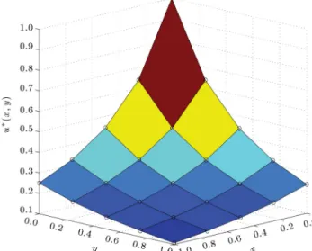
One can compare the approximate and exact solutions of the integral equation in Figures 1 and 2. The error function (Eq. (34)) can be seen in Figure 3. The numerical results are also compared in Table 1. Example 2. As the second example, consider the following integral equation with the exact solution u(x; y) = log1 + xy
(1+y2)
[19]:
u(x; y) = f(x; y) + Z 1
0
Z 1
0 k(x; y; s; t; u(s; t))dtds;
where:
f(x; y) = 16(1 + y)x log
1 + (1 + yxy 2)
;
k(x; y; s; t; u(s; t))=
x(1 t2)
(1 + y)(1 + s2)
Figure 1. The surface of the approximate solution u(x; y) in Example 1.
Figure 2. The surface of the exact solution u(x; y) in Example 1.
Figure 3. The error function e(x; y) in Example 1.
Table 1. The results for Example 1 with (xi; yj) = (4i;j4)(i; j = 0; 1; :::; 4):
(xi; yj) u(xi; yj) u(xi; yj) e(xi; yj)
(0, 0) 1.0000 1.0000 0.0000
(0, 0.25) 0.6400 0.6400 0.0000 (0, 0.5) 0.4444 0.4444 0.0000 (0, 0.75) 0.3265 0.3265 0.0000
(0, 1) 0.2500 0.2500 0.0000
(0.25, 0) 0.6400 0.6400 0.0023 (0.25, 0.25) 0.4426 0.4444 0.0018 (0.25, 0.5) 0.3250 0.3265 0.0015 (0.25, 0.75) 0.24870 0.2500 0.0013 (0.25, 1) 0.1964 0.1975 0.0011 (0.5, 0) 0.4399 0.4444 0.0046 (0.5, 0.25) 0.3229 0.3265 0.0037 (0.5, 0.5) 0.2464 0.2500 0.0031 (0.5, 0.75) 0.1949 0.1975 0.0026 (0.5, 1) 0.1577 0.1600 0.0023 (0.75, 0) 0.3179 0.3265 0.0069 (0.75, 0.25) 0.2445 0.2500 0.0055 (0.75, 0.5) 0.1929 0.1975 0.0046 (0.75, 0.75) 0.1561 0.1600 0.0039 (0.75, 1) 0.1288 0.1322 0.0034
(1, 0) 0.2408 0.2500 0.0092
(1, 0.25) 0.1902 0.1975 0.0073 (1, 0.5) 0.1539 0.1600 0.0061 (1, 0.75) 0.1270 0.1322 0.0052
(1, 1) 0.1065 0.1111 0.0046
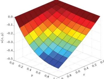
In this example, we choose M = N = 4 and m = n = p = 10: We employe again the LP model (33) and obtain Figures 4 and 5. The error function in Figure 6 also shows the precision of the approximate solution. The numerical results are summarized in Table 2.
To end this section, we answer a natural ques-tion: Are there advantages of our proposed method compared to the existing ones? To answer this, we summarize what we have observed from numerical experiments and theoretical results as below:
Comparison of the results of the above examples with some other methods such as the proposed schemes in [11,15,18,19,25], shows the eciency of this algorithm more clearly. This result is intuitive, since the results of this algorithm depend explicitly on the slack variables of the nal LP problem (32) and (33).
The proposed transformation method in this article can also allow us to transform easily and eciently the dierent kinds of the integral equation problems into an optimization problem.
Table 2. The results for Example 2 with (xi; yj) = (i4;j4)(i; j = 0; 1; :::; 4):
(xi; yj) u(xi; yj) u(xi; yj) e(xi; yj)
(0, 0) 0.0000 0.0000 0.0000
(0, 0.25) 0.0000 0.0000 0.0000 (0, 0.5) 0.0000 0.0000 0.0000 (0, 0.75) 0.0000 0.0000 0.0000
(0, 1) 0.0000 0.0000 0.0000
(0.25, 0) 0.0156 0.0000 -0.0156 (0.25, 0.25) -0.0447 -0.0572 -0.0125 (0.25, 0.5) -0.0849 -0.0953 -0.0104 (0.25, 0.75) -0.1044 -0.1133 -0.0089 (0.25, 1) -0.1100 -0.1178 -0.0078 (0.5, 0) 0.0312 0.0000 -0.0312 (0.5, 0.25) -0.0862 -0.1112 -0.0250 (0.5, 0.5) -0.1615 -0.1823 -0.0280 (0.5, 0.75) -0.1973 -0.2151 -0.0178 (0.5, 1) -0.2075 -0.2231 -0.0156 (0.75, 0) 0.0469 0.0000 -0.0469 (0.75, 0.25) -0.1250 -0.1625 -0.0375 (0.75, 0.5) -0.2311 -0.2624 -0.0312 (0.75, 0.75) -0.2807 -0.3075 -0.0268 (0.75, 1) -0.2950 -0.3185 -0.0234 (1, 0) 0.0625 0.0000 -0.0625 (1, 0.25) -0.1613 -0.2113 -0.0500 (1, 0.5) -0.2948 -0.3365 -0.0416 (1, 0.75) -0.3563 -0.3920 -0.0357 (1, 1) -0.3742 -0.4055 -0.0312
Figure 4. The surface of the approximate solution u(x; y) in Example 2.
Since the procedure of this algorithm is not iterative and does not need any initial guess of the solution, subsequently, appears that the applied method in this paper is very easy to use and straightforward in comparison with other numerical methods.
Figure 5. The surface of the exact solution u(x; y) in Example 2.
Figure 6. The error function e(x; y) in Example 2.
6. Conclusion
In this paper, we investigated an optimization tech-nique for solving two dimensional nonlinear Fredholm integral equations of the second kind. The integral equation problem was transformed into an approximat-ing optimization problem, and the embeddapproximat-ing method based on some principles of measure theory, func-tional analysis and linear programming was applied for solving this integral equation. The method is not iterative and it does not need any initial guess of the solution. Furthermore, in this approach the nonlinearity of the continuous kernels has not serious eects on the solution.
References
1. Bloom, F. \Asymptotic bounds for solutions to a system of damped integro-dierential equations of electromagnetic theory", J. Math. Anal. Appl., 73, pp. 524-542 (1980).
2. Holmaker, K. \Global asymptotic stability for a sta-tionary solution of a system of integro-dierential equations describing the formation of liver zones", SIAM J. Math. Anal., 24(1), pp. 116-128 (1993). 3. Abdou, M.A. \On asymptotic methods for Fredholm{
Volterra integral equation of the second kind in contact problems", J. Comput. Appl. Math., 154, pp. 431-446 (2003).
4. Forbes, L.K., Crozier, S. and Doddrell, D.M. \Calcu-lating current densities and elds produced by shielded magnetic resonance imaging probes", SIAM J. Appl. Math., 57(2), pp. 401-425 (1997).
5. Polyanin, A.D. and Manzhirov, A.V., Handbook of Integral Equations, 2nd Ed., Chapman & Hall/CRC Press, Boca Raton, 2008, Updated, Revised and Ex-tended.
6. Golberg, M.A. \The convergence of a collocations method for a class of Cauchy singular integral equa-tions", J. Math. Appl., 100, pp. 500-512 (1984). 7. Kovalenko, E.V. \Some approximate methods for
solving integral equations of mixed problems", Provl. Math. Mech., 53(1), pp. 85-92 (1989).
8. Semetanian, B.J. \On an integral equation for axially symmetric problem in the case of an elastic body containing an inclusion", J. Appl. Math. Mech., 55(3), pp. 371-375 (1991).
9. Willis, J.R. and Nemat-Nasser, S. \Singular perturba-tion soluperturba-tion of a class of singular integral equaperturba-tions", Quart. Appl. Math., XLVIII(4), pp. 741-753 (1990). 10. Frankel, J. \A Galerkin solution to regularized Cauchy
singular integro-dierential equation", Quart. Appl. Math., 52(2), pp. 145-258 (1995).
11. Alipanah, A. and Esmaeili, S. \Numerical solution of the two-dimensional Fredholm integral equations using Gaussian radial basis function", J. Comput. Appl. Math., 235, pp. 5342-5347 (2011).
12. Atkinson, K.E., A Survey of Numerical Methods for the Solution of Fredholm Integral Equations of the Second Kind, Philadelphia: SIAM (1976).
13. Atkinson, K.E., The Numerical Solution of Integral Equations of the Second Kind, Cambridge University Press (2011).
14. Borzabadi, A.H. and Fard, O.S. \A numerical scheme for a class of nonlinear Fredholm integral equations of the second kind", J. Comput. Appl. Math., 232, pp. 449-454 (2009).
15. Babolian, E., Bazm, S. and Lima, P. \Numerical solution of nonlinear two-dimensional integral equa-tions using rationalized Haar funcequa-tions", Commun. Nonlinear Sci. Numer. Simulat., 16, pp. 1164-1175 (2011).
16. Baker, C.T., Numerical Treatment of Integral Equa-tions, Clarendon Press: Oxford (1977).
17. Delves, L.M. and Mohamed, J.L. Computational Methods for Integral Equations, Cambridge University Press (2011).
18. Han, G. and Wang, R. \Richardson extrapolation of iterated discrete Galerkin solution for two-dimensional Fredholm integral equations", J. Comput. Appl. Math., 139, pp. 49-63 (2002).
19. Han, G.Q. and Jiong, W. \Extrapolation of Nystrom solution for two dimensional nonlinear Fredholm in-tegral equations", J. Comput. Appl. Math., 134, pp. 259-268 (2001).
20. Hetmaniok, E., Slota, D. and Witula, R. \Conver-gence and error estimation of homotopy perturbation method for Fredholm and Volterra integral equations", Appl. Math. Comput., 218, pp. 10717-10725 (2012). 21. Hsiao, C.H. \Hybrid function method for solving
Fredholm and Volterra integral equations of the second kind", J. Comput. Appl. Math., 230, pp. 59-68 (2009). 22. Izzo, G., Jackiewicz, Z., Messina, E. and Vecchio, A. \General linear methods for Volterra integral equa-tions", J. Comput. Appl. Math., 234, pp. 2768-2782 (2010).
23. Izzo, G., Russo, E. and Chiapparelli, C. \Highly stable Runge-Kutta methods for Volterra integral equations", Appl. Numer. Math., 62, pp. 1002-1013 (2012). 24. Reihani, M.H. and Abadi, Z. \Rationalized Haar
functions method for solving Fredholm and Volterra integral equations", J. Comput. Appl. Math., 200, pp. 12-20 (2007).
25. Xie, W.J. and Lin, F.R. \A fast numerical solution method for two dimensional Fredholm integral equa-tions of the second kind", Appl. Numer. Math., 59, pp. 1709-1719 (2009).
26. Rubio, J.E., Control and Optimization; The Linear Treatment of Non-linear Problems, Manchester Uni-versity Press: Manchester U.K. (1986).
27. Rubio, J.E. \The global control of nonlinear diusion equations", SIAM J. Control Optim., 33, pp. 308-322 (1995).
28. Nazemi, A.R., Farahi, M.H. and Zamirian, M. \Fil-tration problem in inhomogeneous dam by using em-bedding method", J. Appl. Math. Comput., 28, pp. 313-332 (2008).
29. Nazemi, A.R., Farahi, M.H. and Mehne, H.H. \Opti-mal shape design of iron pole section of electromag-net", J. Phys. Lett. A, 372, pp. 3440-3451 (2008). 30. Nazemi, A.R. \LP Modelling for the time optimal
control problem of the heat equation", J. Math. Model. Algorithms, 10, pp. 227-244 (2011).
31. Eati, S., Nazemi, A.R. and Shabani, H. \Time optimal control problem of the heat equation with thermal source", IMA J. Math. Control Info., Doi: 10.1093/imamci/dnt016 (2013).
32. Nazemi, A.R. and Eati, S. \Time optimal control problem of the wave equation", J. Adv. Model. Optim., 12, pp. 363-382 (2010).
33. Nazemi, A.R. and Farahi, M.H. \Control the bre orientation distribution at the outlet of contraction", J. Acta Appl. Math., 106, pp. 279-292 (2009). 34. Farahi, M.H., Mehne, H.H. and Borzabadi, A.H.
\Wing drag minimization by using measure theory", Optim. Meth. Soft., 21, pp. 169-177 (2006).
35. Farahi, M.H., Borzabadi, A.H., Mehne, H.H. and Kamyad, A.V. \Measure theoretical approach for opti-mal shape design of a nozzle", J. Appl. Math. Comput., 17, pp. 315-328 (2005).
36. Mehne, H.H., Farahi, M.H. and Esfahani, J.A. \On solving constrained shape optimization problems for nding the optimum shape of a bar cross-section", Appl. Numer. Math., 168, pp. 1258-1272 (2005). 37. Mehne, H.H., Farahi, M.H. and Kamyad, A.V. \MILP
modelling for the time optimal control problem in the
case of multiple targets", Optim. Control Appl. Meth., 27, pp. 77-91 (2006).
38. Rudin, W., Functional Analysis. McGraw-Hill: New York (1991).
39. Rosenbloom, P.C. \Quelques classes de problems ex-tremaux", Bulletin de la Societe Mathematique de France, 80, pp. 183-216 (1952).
Biography
Alireza Nazemi received his BSc degree from Sharif University of Technology, Tehran, Iran, in 2001, his MSc degree from Hakim Sabzevari University, Sabze-var, Iran, in 2003, and his PhD degree from Ferdowsi University of Mashhad, Mashhad, Iran, in 2008, all in applied mathematics. He is currently an Associate Professor at University of Shahrood, Iran. His current research interests include control and optimization, distributed parameter systems, and neural network theory.