ISSN: 2252-8938, DOI: 10.11591/ijai.v9.i1.pp33-39 33
Artificial neural network forecasting performance with missing
value imputations
Nur Haizum Abd Rahman1, Muhammad Hisyam Lee2
1Department of Mathematics, Faculty of Science, Universiti Putra Malaysia, 43400, Serdang, Selangor, Malaysia 2Department of Mathematical Sciences, Faculty of Science, Universiti Teknologi Malaysia, 81310, Skudai, Johor Bahru,
Johor, Malaysia
Article Info ABSTRACT
Article history: Received Nov 12, 2019 Revised Jan 25, 2020 Accepted Feb 2, 2020
This paper presents time series forecasting method in order to achieve high accuracy performance. In this study, the modern time series approach with the presence of missing values problem is developed. The artificial neural networks (ANNs) is used to forecast the future values with the missing value imputations methods used known as average, normal ratio and also the modified method. The results are validated by using mean absolute error (MAE) and root mean square error (RMSE). The result shown that by considering the right method in missing values problems can improved artificial neural network forecast accuracy. It is proven in both MAE and RMSE measurements as forecast improved from 8.75 to 4.56 and from 10.57 to 5.85 respectively. Thus, this study suggests by understanding the problem in time series data can produce accurate forecast and the correct decision making can be produced.
Keywords:
Air pollutant index Error measurements
Artificial neural network Imputations
Forecating
This is an open access article under the CC BY-SA license.
Corresponding Author: Nur Haizum Abd Rahman, Department of Mathematics,
Faculty of Science, Universiti Putra Malaysia, 43400, Serdang, Selangor, Malaysia.
Email: [email protected]
1. INTRODUCTION
Data can be obtain according to time either in hourly, daily or yearly. This form of recorded data is know as time series. By analysis the time series data, the structure of the data can be taken in building the model [1]. Many forecasting techniques have been reported in the literature [2]. In general, these techniques can be classified roughly into three groups, i.e. statistical modified-classical methods, techniques based on artificial intelligences, and advanced techniques.
The most important classical method is the autoregressive integrated moving average (ARIMA) model because of its flexibility in modelling different types of dataset [1, 3]. This model is executed from the autoregressive model (AR), the moving average model (MA) and the combination of AR and MA models, which is known as ARMA models. In addition, if there is an existence of seasonal component in the series, then the model is known as seasonal ARIMA (SARIMA) model [3]. Thus, the flexibility of this model make it competitive with the recently developed methods. However, the major limitation of this model is that it can only capture the linear form of time series data and the preliminary analysis stages become the constraint in building this model [4].
As an alternative to the classical methods, forecasters have developed new methods that can overcome the limitation of classical methods, such as artificial neural network (ANN) and the fuzzy time series (FTS). ANN has been widely used as a forecasting model in many applications [5]. This include
weather forecast [6], electricity price [7], airline data [8], and many others. It is because ANN is flexible in forecasting applications since it can model both linear and non-linear processes [9]. In developing ANN model, the pre-processing of data is important before analysis where the data transformation normally used is [-1, 1] or [0, 1] [10-12]. Different from previous study, the analysis take the important of imputation the missing data into ANN forecast. The forecast performance will be validate using real data which is air quality data.
Air pollution is the major pollution problem in the world [13]. Power production from power plant, vehicles fuel burning, industrial processes and natural factors like volcano eruption make the air quality worsen. The issues of air quality now become a major concern worldwide as its effects are diverse and numerous [14]. The pollution not only effect human health but also towards the forests, waters and whole ecosystem.
In Malaysia, a series of haze episodes were reported since the 1980s [15]. Massive land and forest fires in Sumatra and Kalimantan, Indonesia has been the main reason of haze episodes occurrence. The winds has made it easier for the heavy haze to be transported. According to DOE report [16], for the first time in Malaysia’s history, 34 stations in this country recorded unhealthy air quality status which happened on 15 September 2015. Besides Malaysia, haze also reaches another Southeast Asia country such as Singapore, Thailand and Brunei [17].
The Department of Environment (DOE) is a government agency which is responsible to monitor and manage Malaysia’s air quality. Thus, to identify and give information on the severity of air pollution to the public, the ambient air quality measurement in Malaysia is described in terms of Air Pollutant Index (API). Based on the average of main pollutants namely sulphur dioxide (SO2), nitrogen dioxide (NO2), carbon monoxide (CO), ozone (O2), particulate matter diameter 2.5 (PM2.5) and particulate matter diameter 10 (PM10), the API value is measured. The highest pollutant’s concentration will determine the API value. Usually, PM2.5 is the highest concentration recorded compared to other pollutants.
Air quality data has been recorded in Malaysia since 1996 and the huge amount of data usually presented in the form of text information. Thus, air quality information are difficult to be reviewed, especially for the public understanding. Moreover, the public, especially those in high risk groups such as asthmatic individuals, children, and elderly, need to be alerted beforehand about the cases of poor air quality. Therefore, this study use time series approach by using classical and modern methods which are Box-Jenkins and ANN to solve forecast accuracy issued with the presence of missing data. It is important to implement air quality management and public warning strategies for pollution levels that are acceptable to the public.
2. RESEARCH METHOD
2.1. Box-Jenkins method
Box-Jenkins method or autoregressive integrated moving average (ARIMA) method was first introduced by Box and Jenkins [18]. Originated from the autoregressive model (AR), the moving average model (MA) and differencing order of d known as the integrated (I) model. The seasonal ARIMA model (SARIMA) is used when the seasonal components are included in this ARIMA model. The generalized form of SARIMA (p, d, q)(P, D, Q)S model can be written as:
𝜙𝑝(𝐵)𝛷𝑝(𝐵𝑆)(1 − 𝐵)𝑑(1 − 𝐵𝑆)𝐷𝑌𝑡= 𝜃𝑞(𝐵)𝛩𝑞(𝐵𝑆)𝑎𝑡 (1)
where
𝜙𝑝(𝐵) = 1 − 𝜙1𝐵 − 𝜙2𝐵2− ⋯ − 𝜙𝑝𝐵𝑝
𝛷𝑃(𝐵) = 1 − 𝛷1𝐵𝑆− 𝛷2𝐵2𝑆− ⋯ − 𝛷𝑃𝐵𝑃𝑆
𝜃𝑞(𝐵) = 1 − 𝜃1𝐵 − 𝜃2𝐵2− ⋯ − 𝜃𝑝𝐵𝑝
𝛩𝑄(𝐵) = 1 − 𝛩1𝐵𝑆− 𝛩2𝐵2𝑆− ⋯ − 𝛩𝑄𝐵𝑄𝑆
B is denoted as the backward shift operator, d and D are denoted as the non-seasonal and seasonal orders of difference respectively. Box-Jenkins procedure contains three main stages to build an ARIMA model, i.e. model identification, model estimation and model checking.
2.2. Artificial neural network
Artificial neural network (ANN) is one of the artificial intelligence approaches. It is one of the most accurate and widely used forecasting methods. Multi-layer perceptron (MLP) or also known as the feed-forward neural network (FFNN) is broadly used as ANN approach [10, 12]. The term perceptron refers to the
simplest form of a neural network used for the classification. Generally, the components of ANN are neuron, layer, activation function and weight.
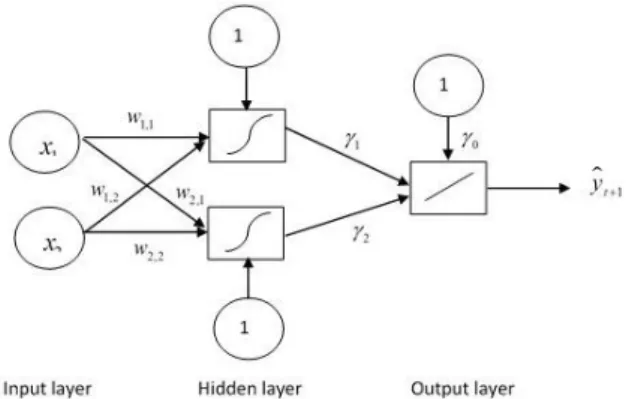
MLP consists of three layers i.e. input layer, hidden layer and output layer [19] as shown in Figure 1. Each input node in the input layer will be forwarded to the neurons with the arrival of a certain weight [20]. Input will be processed by a backpropagation function which will add up the values of all weights. This sum will be compared with a threshold value given by the activation function of each neuron. Commonly, in the hidden layer, the activation function used is the logistic function, 𝑓(𝑥) = 1/(1 − exp(−𝑥)), meanwhile the linear function, 𝑓(𝑥) = 𝑥, is used at the output stage. If the input is passed a certain threshold, then the neuron will be activated. When the neurons are activated, the neuron will transmit output via the output weights to all neurons associated with it. There are constants or bias (in NN jargon) connected to each neurons and output, denoted as one [8].
Figure 1. Neural network architecture example with two inputs and two neurons.
MLP is trained by back propagation learning which is capable to solve more complex problems compared with single layer nets and outliers [21]. This procedure repeatedly modifies the weights on the connection links in a NN so that it minimizes the difference between actual output and the desired output. MLP model in statistics modelling for time series forecasting can be considered as a non-linear autoregressive (AR) model. In time series forecasting, the input node is the lag(s) of available historical data determined based on the autoregressive order in the Box-Jenkins model [8, 5].
Based on Figure 1, the MLP relationship between the output 𝑦𝑡and the inputs, 𝑥𝑡−1, 𝑥𝑡−2, . . . , 𝑥𝑡−𝑛
has the following mathematical representation: 𝑦𝑖= 𝑤0+ ∑ 𝑤𝑖𝑥𝑗
𝑛
𝑖=1 (2)
𝑦𝑡= 𝑤0+ ∑ 𝑤𝑗𝑔(𝑤0𝑗+
𝑞
𝑗=1 ∑ 𝑤𝑖𝑗𝑥𝑡−𝑖+
𝑝
𝑖=1 𝑎𝑡) (3)
where 𝑤𝑗; (𝑗 = 1, 2, . . , 𝑞) and 𝑤𝑖𝑗 (𝑖 = 1, 2, . . . , 𝑝; 𝑗 = 1, 2, . . . , 𝑞) are the model parameters that are often
called as the connection weights; p is the number of input nodes and q is the number of hidden nodes. 2.3. Missing values imputation
2.3.1. Decomposition method
The basic idea for the decomposition method is to decompose the problem into sub problems, which is used as the solution for various problems and algorithms. The sub problems are trend, seasonal, cyclical and irregular (error). The estimates from these factors are used to describe the series and can be used to compute point forecasts. This method can be presented into two forms; an additive decomposition and multiplicative decomposition. The equation of both forms with the factors can be presented as below. Additive decomposition:
𝑌𝑡 = 𝑇𝑡 + 𝑆𝑡 + 𝐶𝑡 + 𝐼𝑡 (4)
𝑌𝑡 = 𝑇𝑡 × 𝑆𝑡 × 𝐶𝑡 × 𝐼𝑡 (5)
where 𝑇𝑡, 𝑆𝑡, 𝐶𝑡 and 𝐼𝑡 are trend, seasonal, cyclic and irregular at time respectively.
2.3.2. Spatial weighting method
The analysis of missing values using the spatial weighting methods will involve a target station with selected neighboring stations. Generally, the weighting method formula is given as follows:
𝑌̂𝑡= ∑𝑁𝑖=1𝑊𝑖𝑌𝑖 𝑡≠𝑖
(6)
where 𝑌𝑖 is the estimated value of the missing data at the target station, 𝑡 (𝑡 ≠ 𝑖), N is the number of
neighboring stations, 𝑌𝑖 is the observation at theith neighboring station and 𝑊𝑖 is the weight of the ith
neighboring station with constraint 𝑊𝑖= 1.
The arithmetic average (AA) method is the classically way to identify weight. It considered equal weight for each selected neighboring station. It can be defined as:
𝑊𝑖=
1
𝑁 (7)
The second method is the normal ratio (NR) method. The NR method was firstly proposed by [22]. The method is based on the mean ratio of available data between the target station, and the ith neighboring stations. The method is given as follows:
𝑊𝑖=
1 𝑁∑
𝜇𝑡
𝜇𝑖 𝑁
𝑖=1 (8)
where µ𝑡 and µ𝑖 are the sample mean of the available data at the target station 𝑡, and the ith neighboring
stations respectively.
In 1992, Young proposed to use the correlation between the target station and the neighboring station as the weighting factors [23]. The weight known as the modified normal ratio based on correlation (MNR) is given as follows:
𝑊𝑖=
(𝑛𝑖−2)𝑟𝑖𝑡2(1−𝑟𝑖𝑡2)−1 ∑𝑁 (𝑛𝑖−2)𝑟𝑖𝑡2(1−𝑟𝑖𝑡2)−1
𝑖=1
(9)
where 𝑟𝑖𝑡 is the correlation coefficient of the daily time series data between the target station and the ith
neighboring stations, 𝑛𝑖 is the length of data series that are used to compute the correlation coefficient.
2.4. Error measurement
Let 𝑦𝑡 be the actual values, 𝑦̂𝑡 is the forecast values and 𝑡 is time. Thus, the error be defined as, 𝑒𝑡=
𝑦𝑡− 𝑦̂𝑡. The measurements used in this study are mean absolute error (MAE) and root mean square error
(RMSE). The equation for both measurements as follow: MAE=∑𝑛𝑡=1|𝑦𝑡−𝑦̂𝑡|
𝑛 (10)
RMSE=√∑𝑛𝑡=1(𝑦𝑡−𝑦̂𝑡)2
𝑛 (11)
The MAE and RMSE are scale dependent measure where both not suitable to compare the forecast with different scale. Both of these measurements are easy to interpret since the error can be computed directly from the actual and forecast values without involving any unknown parameter that needs to be estimated [24].
3. RESULTS AND DISCUSSION
The analyses of API data are presented in this section. Station located in Johor Bahru city was chosen for this study since it is the capital of Johor state and the second largest metropolitan in Malaysia. Thus, it is home to a large number of the region’s industries, residential, and commercial hotspots. The study
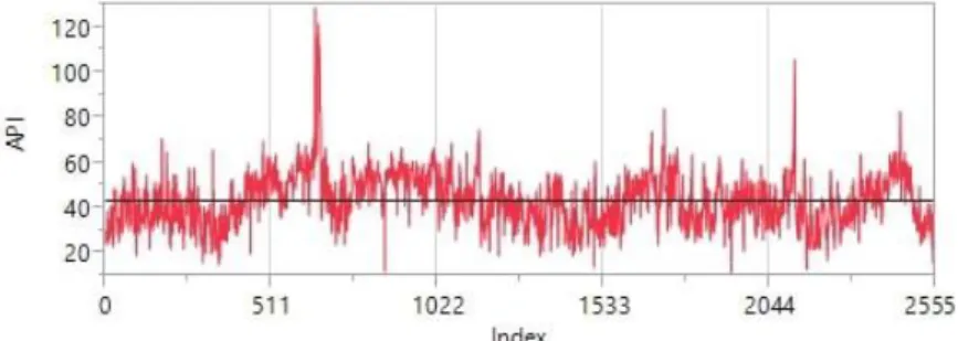
used daily data set for seven years, from year 2005 until 2011. The data were divided into two data sets: (1) a training set from 2005 until 2010 with total of 2191 observations to find the suitable API model, and (2) a test data set in year 2011 with a total of 365 observations to check the model performance. The missing data were initially estimated by using the decomposition method. Figure 2 show the time series plot for both training and testing data set.
Figure 2. Time series plot for daily API in Johor Bahru
From Figure 2, the API series consist yearly seasonality where the data start to increase in the middle of the year. The seasonality indicate nonstationary data. Thus, the data transformation and differencing in both seasonal and nonseasonal were carried out to obtain stationary series.
There were two possible models showed significant result in both parameter and L-jung Box statistics, which were SARIMA(3, 1, 3)(0, 1, 1)365 and SARIMA(3, 1, 3)(2, 1, 0)365. Comparing both models in
terms of RMSE, the SARIMA(3, 1, 3)(0, 1, 1)365 was the best model to forecast the daily data because of the
lowest RMSE value, 10.52.
The data pre-processing for ANN method used in Johor Bahru daily API data included the normalize data transformation and scaled interval transformation of [0,1] and [-1,1]. In input layer, the input nodes were identified based on all lags from the best SARIMA model (SARIMA(3, 1, 3)(0, 1, 1)365), seasonal
lags which are 365 and 730 and lastly lag 1 with before and after seasonal lags (1, 364, 365, 366, 729, 730 and 731). Table 1 showed that the smallest RMSE with value of 10.57 was by using all input lags from the best SARIMA model with the data transformation of [-1,1].
Missing data or incomplete data matrices is a problem that is repeatedly encountered in many areas, including the environmental research. This is common and unavoidable problem caused by unsystematic data storing, instrument malfunctions, and stations relocation [25]. Missing data can lead to insufficient data sampling, errors in measurements, and it gives a significant effect to the conclusions that could be drawn from the data [26]. In time series, the analysis requires the data to be continuously available. Thus, an appropriate statistical method is important to solve the missing data problem.
Table 1. ANN forecasting accuracy based on RMSE for daily API in Johor Bahru
Lags Normalize [0,1] [-1,1]
All 10.57 10.64 10.57
Seasonal (365,730) 10.99 10.90 10.99
Lag 1 with seasonal lags ± 1
11.06 11.07 11.06
The spatial weighting method was used since numbers of monitoring stations were available near to the selected stations. Imputation methods were tested in different distances, 100 km, 150 km, and 200 km in order to test the method’s sensitivity so that optimal result can be produced.
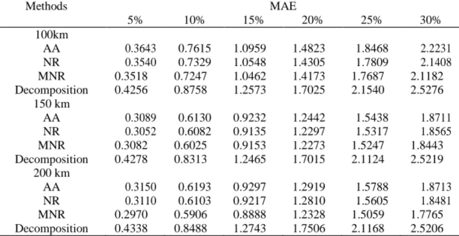
To check the stability of the method, six different percentage ranges from 5% to 30% were chosen. Performance of the imputation methods are compared by using MAE measurement. Lowest MAE indicate better imputation. As shown in Table 2, in 100 km distance, MNR was the best method in all percentage missing. In 150 km distance, the result varied between old normal ratio, NR and modified normal ratio, MNR. The best imputation for NR were in 5% and 15% percentage missing, while for MNR, the best imputation were in 10%, 20%, 25%, and 30% percentage missing. Consistent result also obtained in 200 km as it indicated that the MNR was the best imputation method. Thus, as conclusion MNR was the best method while decomposition was the worst method.
Table 2. Performance missing values estimation based on MAE
Methods MAE
5% 10% 15% 20% 25% 30%
100km
AA 0.3643 0.7615 1.0959 1.4823 1.8468 2.2231
NR 0.3540 0.7329 1.0548 1.4305 1.7809 2.1408
MNR Decomposition 0.3518 0.4256 0.7247 0.8758 1.0462 1.2573 1.4173 1.7025 1.7687 2.1540 2.1182 2.5276 150 km
AA 0.3089 0.6130 0.9232 1.2442 1.5438 1.8711
NR 0.3052 0.6082 0.9135 1.2297 1.5317 1.8565
MNR Decomposition 0.3082 0.4278 0.6025 0.8313 0.9153 1.2465 1.2273 1.7015 1.5247 2.1124 1.8443 2.5219 200 km
AA 0.3150 0.6193 0.9297 1.2919 1.5788 1.8713
NR 0.3110 0.6103 0.9217 1.2810 1.5605 1.8481
MNR Decomposition 0.2970 0.4338 0.5906 0.8488 0.8888 1.2743 1.2328 1.7506 1.5059 2.1168 1.7765 2.5206
The similar processes are conducted after missing values imputation performed. The new performance evaluations were given in Table 3. The result shown that the ANN model can outperformed SARIMA model and improved the forecasting performance. The MAE improved from 8.75 to 4.56 and RMSE from 10.57 to 5.85.
Table 3. Performance evaluation for daily API
Imputation Method Forecasting Method MAE RMSE
Decompositon SARIMA 8.37 10.52
ANN 8.75 10.57
MNR SARIMA 8.44 10.63
ANN 4.56 5.85
4. CONCLUSION
This paper presents the problem of how to forecast the huge amount of API dataset contaminated with different ranges of the API scales and terms that used in assessing and describing the air quality status on human health. The objective of the study was to adapt time series method, classical method and modern method that would yield satisfactory workable results for the API forecasts with missing data problem. From the result, it is evident that the modern method, artificial neural network (ANN) gave better forecasting performances in forecasting compared to SARIMA model. Besides, ANN showed improvement in forecasting after high accuracy data imputation conducted. The ability of ANN to capture complex data pattern which consist both linear and nonlinear make the reason for the good performance of ANN model [9]. For future recommendation, this study can be extend with input from the other pollutant in target and neighboring stations.
ACKNOWLEDGEMENTS
This study was supported by Universiti Putra Malaysia, Malaysia under Putra-IPM grant, 9587700. We would like to thanks the Department of Environment (DOE), Malaysia for providing air pollutants data.
REFERENCES
[1] J. D. Cryer and K. S. Chan, Time Series Analysis: with Applications in R. New York: Springer-Verlag New York Inc., 2010, pp. 1-141.
[2] J. G. D. Gooijer and R. J. Hyndman, “25 Years of Time series Forecasting,” International Journal of Forecasting, vol. 22, Issue 3, pp. 443-473, 2006.
[3] S. Suhartono, “Time Series Forecasting by using Seasonal Autoregressive Integrated Moving Average: Subset, Multiplicative or Additive Model,” Journal of Mathematics and Statistics, vol. 7, pp. 20-27, 2011.
[4] M. E. Nor, et al., “Fuzzy Time Series and SARIMA Model for Forecasting Tourist Arrivals to Bali,” Jurnal Teknologi (Sciences and Engineering), vol. 57, pp. 69-81, 2012.
[5] G. Zhang, B. E. Patuwo and M. Y. Hu, “Forecasting with Artificial Neural Networks: The State of the Art,”
[6] K. Abhishek, et al., “Weather Forecasting Model using Artificial Neural Network,” Procedia Technology, vol. 4, pp. 311-318, 2012.
[7] I. P. Panapakidis and A. S. Dagoumas, “Day-Ahead Electricity Price Forecasting via the Application of Artificial Neural Network based Models,” Applied Energy, vol. 172, pp. 132-151, 2016.
[8] J. Faraway and C. Chatfield, “Time Series Forecasting with Neural Networks: A Comparative Study using the Airline Data,” Applied Statistics, vol. 47, pp. 231-250, 1998.
[9] S. Barhmi and O. E. Fatni, “Hourly Wind Speed Forecasting based on Support Vector Machine and Artificial Neural Networks,” International Journal of Artificial Intelligence, vol. 8, pp. 286-291, 2019.
[10] W. S. Sarle, “Neural Networks and Statistical Models,” Proceedings of the Nineteenth Annual SAS Users Group International Conference, 1994.
[11] J. J. Shi, “Reducing Prediction Error by Tansforming Input Data for Neural Networks,” Journal of Computing in Civil Engineering, vol. 14, pp. 109-116, 2000.
[12] A. Palmer, J. J. Montano, and A. Sese, “Designing an Artificial Neural Network for Forecasting Tourism Time Series,” Tourism Management, vol. 27, pp. 781-790, 2006.
[13] A. Kurt and A. B. Oktay, “Forecasting Air Pollutant Indicator Levels with Geographic Models 3 Days in Advance using Neural Networks,” Expert Systems with Applications, vol. 37, Issue 12, pp. 7986-7992, 2010.
[14] Z. Yang and J. Wang, “A New Air Quality Monitoring and Early Warning System: Air Quality Assessment and Air Pollutant Concentration Prediction,” Environmental Research, vol. 158, pp. 105-117, 2017.
[15] R. Afroz, M. N. Hassan, and N. A. Ibrahim “Review of Air Pollution and Health Impacts in Malaysia,”
Environmental Research, vol. 92, pp. 71-77, 2003.
[16] Department of Environment, “Chronology of Haze Episodes in Malaysia,” Putrajaya: Department of Environment. [17] N. H. A. Rahman, M. H. Lee, S. Suhartono and M. T. Latif, “Evaluation Performance of Time Series Approach for
Forecasting Air Pollution Index in Johor, Malaysia,” Sains Malaysiana, vol. 45, pp. 1625–1633, 2016.
[18] M. Khashei and M. Bijari, “A Novel Hybridization of Artificial Neural Networks and ARIMA Models for Time Series Forecasting,” Applied Soft Computing Journal, vol. 11, pp. 2664-2675, 2011.
[19] F. Yumono, et al., “Artificial Neural Network for Healthy Chicken Meat Identification,” International Journal of Artificial Intelligence, vol. 7, pp. 63-70, 2018.
[20] K. C. Rani and Y. Prasanth, “A Decision System for Predicting Diabetes using Neural Networks,” International Journal of Artificial Intelligence, vol. 6, pp. 56-65, 2017.
[21] R. Law, “Back-Propagation Learning in Improving the Accuracy of Neural Network-Based Tourism Demand Forecasting,” Tourism Management, vol. 21, pp. 331-340, 2000.
[22] J. L. H. Paulhus and M. A. Kohler, “Interpolation of Missing Precipitation Records,” Monthly Weather Review, vol. 80, pp. 129-133, 1952.
[23] K. C. Young, “A Three-Way Model for Interpolating for Monthly Precipitation Values,” Monthly Weather Review, vol. 120, pp. 2561-2569, 1992.
[24] G. Elliott, I. Komunjer and A. Timmerman, “Estimation and Testing of Forecast Rationality under Flexible Loss,”
Review of Economic Studies, vol. 72, pp. 1107-1125, 2005.
[25] H. Junninen, et al., ”Methods for Imputation of Missing Values in Air Quality Data Sets,” Atmospheric Environment, vol. 38, pp. 2895-2907, 2004.
[26] J. Suhaila, M. D. Sayang, and A. A. Jemain, “Revised Spatial Weighting Methods for Estimation of Missing Rainfall Data,” Asia-Pacific Journal of Atmospheric Sciences, vol. 44, pp. 93-104, 2008.