HIGH-PRECISION EXTREME-MASS-RATIO INSPIRALS IN BLACK HOLE PERTURBATION THEORY AND POST-NEWTONIAN THEORY
Erik Robert Forseth
A dissertation submitted to the faculty at the University of North Carolina at Chapel Hill in partial fulfillment of the requirements for the degree of Doctor of Philosophy in the Department of Physics &
Astronomy.
Chapel Hill 2016
ABSTRACT
Erik Robert Forseth: High-precision extreme-mass-ratio inspirals in black hole perturbation theory and post-Newtonian theory
(Under the direction of Charles R. Evans)
The recent detection of gravitational wave (GW) signal GW150914 by the Advanced LIGO experiment inaugurated the long-anticipated era of GW astronomy. This event saw the merger of two black holes, having roughly 36 and 29 solar masses, and the ringdown of the resulting 62 solar mass black hole. The energy emitted in gravitational radiation was equivalent to about three solar masses. The detection underscored the importance of theoretical models for not only isolating signal from noise, but especially for the accurate estimation of source parameters. The two-body problem in Einstein’s general theory has no exact solution, and so the development of these models is the subject of intensive research.
We present a set of results for a class of binary systems known as extreme-mass-ratio inspirals (EMRIs), comprised of a small compact object (generically a stellar-mass black hole) in orbit about a supermassive black hole (having∼105
−109solar masses). Our work also has potential application to
intermediate-mass-ratio inspirals (IMRIs), for which the mass intermediate-mass-ratio is 10−4
−10−2. IMRIs are thought to be a potentially strong
source for ground-based GW experiments such as Advanced LIGO/VIRGO. Though not generally a good source for the LIGO network, EMRIs are well-suited for detection by proposed space-based detectors, e.g. eLISA. Our work particularly constitutes a program of developing computational tools, methods, and results foreccentric E/IMRIs, which are thought to be astrophysically important but are much more challenging to model theoretically compared with circular orbits.
ACKNOWLEDGMENTS
Thanks to my family, especially my parents, for their steadfast support, and for the unfailing impression that I’m making them proud.
Thanks to my advisor, Chuck Evans, whose example and direction will last a lifetime. Thanks to Seth Hopper, for his patient help with much of the work presented here.
Finally, thanks to Mononoke and Buddy, for being the two best dogs, and thanks to Mariko, for everything else.
TABLE OF CONTENTS
LIST OF TABLES . . . xi
LIST OF FIGURES . . . xiv
LIST OF CONVENTIONS AND ABBREVIATIONS . . . .xvii
1 Introduction . . . 1
1.1 Gravity as spacetime curvature . . . 1
1.1.1 Mathematical preliminaries . . . 1
1.1.2 Parallel transport and geodesic motion . . . 3
1.1.3 Spacetime curvature and the Riemann tensor . . . 4
1.1.4 Einstein field equations . . . 5
1.1.5 The Schwarzschild black hole solution . . . 6
1.2 The two-body problem in general relativity (GR) . . . 7
1.3 Gravitational radiation and observational interest . . . 8
1.4 Original contributions of this work and organization of document . . . 9
2 BHP and GSF: background and development . . . 11
2.1 Assumptions and applicability . . . 11
2.2 Linearized field equations in flat spacetime . . . 12
2.2.1 Lorenz gauge . . . 14
2.2.2 The plane wave solution and gravitational wave polarizations . . . 15
2.3 Perturbations on curved spacetimes . . . 16
2.4 Self-force . . . 17
2.4.1 Newtonian self-force . . . 18
2.4.3 Gravitational radiation-reaction/self-force . . . 20
3 PN theory: background and development . . . 22
3.1 Assumptions and applicability . . . 22
3.2 Post-Minkowskian approximation . . . 24
3.2.1 Landau-Lifshitz formulation of GR . . . 24
3.2.2 Iterative solution to relaxed field equations . . . 26
3.3 1PN metric, equations of motion . . . 26
3.3.1 PN geodesic equations . . . 28
3.3.2 Systems of isolated PN bodies . . . 29
3.3.3 Binary systems . . . 29
3.4 Gravitational radiation and radiation-reaction for PN sources . . . 30
3.4.1 Quadrupole radiation . . . 30
3.4.2 Radiative losses in two-body systems . . . 31
3.4.3 Radiation-reaction in two-body systems . . . 33
4 BHP and GSF using a Lorenz gauge frequency domain procedure . . . 35
4.1 Formalism . . . 39
4.1.1 Bound orbits on a Schwarzschild background . . . 39
4.1.2 First-order metric perturbation equations in Lorenz gauge . . . 41
4.1.3 Spherical harmonic decomposition . . . 41
4.1.4 Lorenz gauge equations for MP amplitudes . . . 42
4.1.5 Self-force and mode-sum regularization . . . 45
4.1.6 Conservative and dissipative parts of the self-force and first-order changes in orbital constants . . . 48
4.2 Frequency domain techniques for solving coupled systems . . . 49
4.2.1 Fourier decomposition . . . 49
4.2.2 Matrix notation for coupled ODE systems . . . 50
4.2.4 Variation of parameters and extended homogeneous solutions for coupled systems . . . 53
4.3 Numerical algorithm . . . 56
4.3.1 General modes . . . 59
4.3.2 Near-static modes . . . 64
4.3.3 Static modes withl≥2 . . . 67
4.3.4 Low-multipole modes . . . 70
4.4 Additional numerical results . . . 73
4.4.1 GSF results and their accuracies . . . 73
4.4.2 Improving the GSF with energy and angular momentum fluxes and a hybrid approach 78 4.5 Conclusions and future work . . . 82
5 Method of spectral source integrations in BHP theory . . . 84
5.1 Spectral integration of bound orbital motion . . . 86
5.1.1 Geodesic motion and the relativistic anomaly . . . 86
5.1.2 Spectral integration: general considerations . . . 88
5.1.3 Spectral solution of the orbital motion . . . 89
5.2 Spectral source integration in the RWZ formalism . . . 92
5.2.1 The RWZ formalism and EHS method . . . 93
5.2.2 SSI for the normalization coefficients . . . 96
5.2.3 SSI and the midpoint and trapezoidal rules . . . 102
5.3 Spectral source integration in Lorenz gauge . . . 103
5.3.1 Odd-parity Lorenz gauge and EHS . . . 103
5.3.2 Spectral source integration for odd-parity normalization constants . . . 107
5.4 Conclusions . . . 110
6 MST method for high-precision energy fluxes, and comparison with PN theory . . . . 112
6.1 Analytic expansions for homogeneous solutions . . . 114
6.1.2 MST analytic function expansions forRlmω . . . 115
6.1.3 Mapping to RWZ master functions . . . 117
6.2 Solution to the perturbation equations using MST and SSI . . . 118
6.2.1 Bound orbits on a Schwarzschild background . . . 119
6.2.2 Solutions to the TD master equation . . . 120
6.2.3 Normalization coefficients . . . 122
6.3 Preparing the PN expansion for comparison with perturbation theory . . . 123
6.3.1 Known instantaneous energy flux terms . . . 124
6.3.2 Making heads or tails of the hereditary terms . . . 125
6.3.3 Applying asymptotic analysis to determine eccentricity singular factors . . . 131
6.3.4 Using Darwin eccentricityeto mapI(et) andK(et) to ˜I(e) and ˜K(e) . . . 135
6.4 Confirming eccentric-orbit fluxes through 3PN relative order . . . 136
6.4.1 Generating numerical results with the MST code . . . 136
6.4.2 Numerically confirming eccentric-orbit PN results through 3PN order . . . 138
6.5 Determining new PN terms between orders 3.5PN and 7PN . . . 140
6.5.1 A model for the higher-order energy flux . . . 141
6.5.2 Roadmap for fitting the higher-order PN expansion . . . 141
6.5.3 The energy flux through 7PN order . . . 143
6.5.4 Discussion . . . 146
6.6 Conclusions . . . 148
7 MST and PN comparison for energy flux to horizon and angular momentum fluxes . .150
7.1 Energy radiated to infinity . . . 151
7.2 Angular momentum radiated to infinity . . . 151
7.2.1 Current PN theory . . . 151
7.2.2 New terms in the PN expansion for the angular momentum radiated to infinity . . . . 153
7.3 Energy radiated to the black hole horizon . . . 156
7.3.2 New terms in the PN expansion for the energy radiated to the black hole horizon . . . 157
7.4 Angular momentum radiated to the black hole horizon . . . 159
7.4.1 Current PN theory . . . 159
7.4.2 New terms in the PN expansion for the angular momentum radiated to the black hole horizon . . . 159
7.5 Conclusions . . . 161
8 Conclusions and outlook . . . 162
8.1 Summary of original contributions . . . 162
8.2 Outlook and future directions . . . 163
Appendix A BHP AND GSF USING A LORENZ GAUGE FREQUENCY DOMAIN PROCEDURE . . . 165
A.1 Asymptotic boundary conditions . . . 165
A.1.1 Near-horizon even-parity Taylor expansions . . . 165
A.1.2 Near-infinity even-parity asymptotic expansions . . . 168
A.1.3 Near-infinity odd-parity asymptotic expansions . . . 170
A.2 Homogeneous static modes . . . 171
A.2.1 Odd-parity . . . 171
A.2.2 Even-parity . . . 172
A.3 Explicit form of the force termsfα n . . . 176
A.4 Additional self-force values . . . 178
Appendix B METHOD OF SPECTRAL SOURCE INTEGRATIONS IN BHP THEORY181 B.1 Exact Fourier spectrum for dtp/dχas p→ ∞ . . . 181
Appendix C MST METHOD FOR HIGH-PRECISION ENERGY FLUXES, AND COM-PARISON WITH PN THEORY. . . 183
C.1 The mass quadrupole tail at 1PN . . . 183
C.1.1 Details of the flux calculation . . . 183
C.3 Numeric coefficients in the high-order post-Newtonian functions . . . 187
Appendix D MST AND PN COMPARISON FOR ENERGY FLUX TO HORIZON AND ANGULAR MOMENTUM FLUXES . . . .194
D.1 Numeric coefficients in the high-order post-Newtonian functions . . . 194
D.2 Flux expansions using the semi-latus rectum . . . 210
LIST OF TABLES
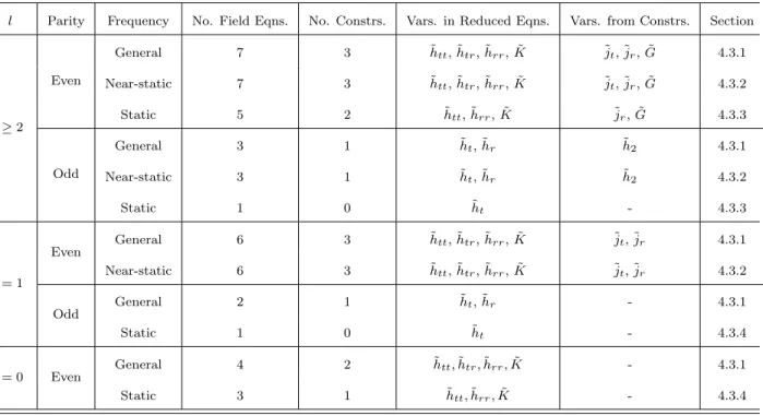
4.1 Classification of FD modes as functions oflmω. Most modes (i.e., general case) are found by solving the complete fully-constrained systems (4.25) and (4.26) and deriving the remaining fields using the gauge conditions (4.23) and (4.24). Special cases include static, near-static, and low-multipole (l = 0,1) modes. For static and low-multipole modes the system size reduces and some MP amplitudes identically vanish. Special cases are discussed in separate
sections as noted. . . 57
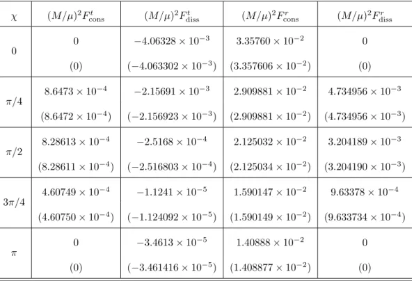
4.2 Comparison of GSF data from two different codes. We give self-force values for an orbit with p = 7.0 and e = 0.2 and present only significant figures for the data from our code (rows without parentheses). Our results are compared to those of Akcay et al. [8] (parentheses), where we have rounded the last digit from values in their table to retain only fully significant digits. Our code took approximately 15 minutes on a single core to generate all of the GSF data in this table. . . 74
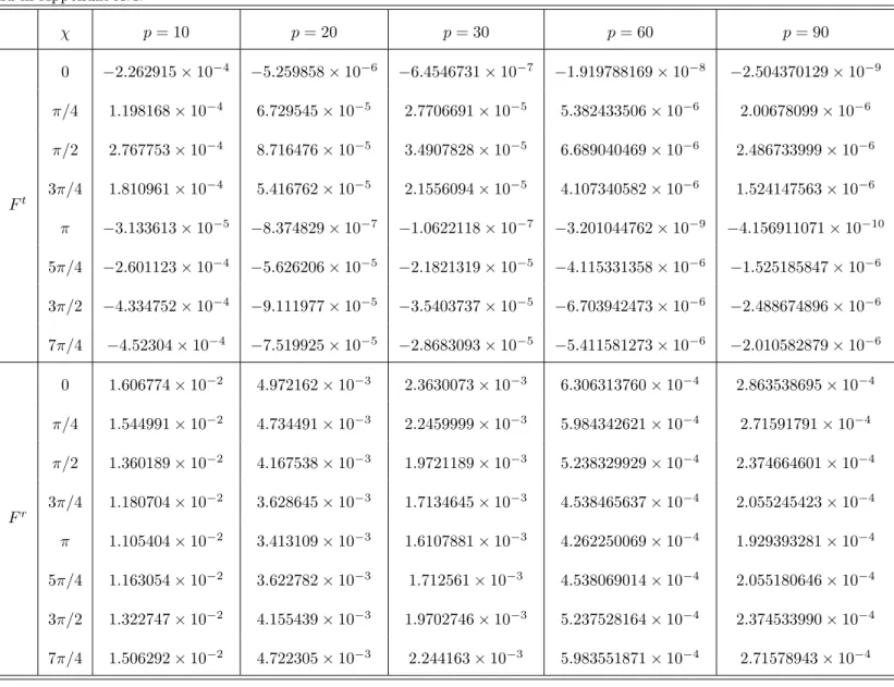
4.3 GSF results for e = 0.1 and a range of p. We present the t and r components of the full regularized self-force at a set of points around a complete radial libration. Dissipative and conservative parts can be obtained by addition or subtraction across conjugate points on the orbit according to Eqns. (4.36). The ϕ component can be recovered from the orthogonal-ity relation Fαu α = 0. Results for additional eccentricities are found in Table 4.4 and in Appendix A.4. . . 76
4.4 Same as Table 4.3 but withe= 0.5. . . 77
4.5 Comparisons of adiabatic contribution forp= 10 . . . 81
A.1 Same as Table 4.3 withe= 0.3. . . 179
A.2 Same as Table 4.3 withe= 0.7. . . 180
C.1 Coefficients in the 3.5PN function according to the form of Eqn. (6.97) for which we were unable to determine rational forms. . . 188
C.2 Coefficients in the 4PN functionL4 according to the form of Eqn. (6.98). . . 188
C.3 Coefficients in the 4.5PN function L9/2 according to the form of Eqn. (6.100). . . 189
C.4 Coefficients in the 4.5PN log function L9/2L according to the form of Eqn. (6.101). . . 189
C.5 Coefficients in the 5PN functionL5 according to the form of equation Eqn. (6.102). . . 190
C.6 Coefficients in the 5PN log functionL5L according to the form of Eqn. (6.103). . . 190
C.7 Coefficients in the 5.5PN function L11/2 according to the form of Eqn. (6.104). . . 191
C.8 Coefficients in the 5.5PN log function L11/2L according to the form of Eqn. (6.105). . . 191
C.9 Coefficients in the 6PN functionL6 according to the form of Eqn. (6.106). . . 192
C.10 Coefficients in the 6PN log functionL6L according to the form of Eqn. (6.107). . . 192
C.11 Coefficients in the 6.5PN function L13/2 according to the form of Eqn. (6.109). . . 192
C.13 Coefficients in the 7PN functionL7 according to the form of Eqn. (6.111). . . 193
C.14 Coefficients in the 7PN log functionL7L according to the form of Eqn. (6.112). . . 193
C.15 Coefficients in the 7PN log-squared function L7L2 according to the form of Eqn. (6.113). . . 193
D.1 Coefficients in the horizon energy flux function B4according to the form of Eqn. (7.49). . . . 195
D.2 Coefficients in the horizon energy flux function B5according to the form of Eqn. (7.51). . . . 196
D.3 Coefficients in the horizon energy flux function B11/2according to the form of Eqn. (7.53). . 196
D.4 Coefficients in the horizon energy flux function B6according to the form of Eqn. (7.54). . . . 197
D.5 Coefficients in the horizon energy flux function B6L according to the form of Eqn. (7.55). . . 197
D.6 Coefficients in the horizon energy flux function B13/2according to the form of Eqn. (7.57). . 198
D.7 Coefficients in the horizon energy flux function B7according to the form of Eqn. (7.58). . . . 198
D.8 Coefficients in the horizon energy flux function B7L according to the form of Eqn. (7.59). . . 198
D.9 Coefficients in the horizon energy flux function B7L2 according to the form of Eqn. (7.60). . 198 D.10 Coefficients in the 3.5PN angular momentum function according to the form of Eqn. (7.22). 199 D.11 Coefficients in the 4PN angular momentum function according to the form of Eqn. (7.23). . 199 D.12 Coefficients in the 4.5PN angular momentum function according to the form of Eqn. (7.25). 200 D.13 Coefficients in the 4.5PN angular momentum log function according to the form of Eqn. (7.26). 200 D.14 Coefficients in the 5PN angular momentum function according to the form of Eqn. (7.27). . 201 D.15 Coefficients in the 5PN angular momentum log function according to the form of Eqn. (7.28). 201 D.16 Coefficients in the 5.5PN angular momentum function according to the form of Eqn. (7.29). 202 D.17 Coefficients in the 5.5PN angular momentum log function according to the form of Eqn. (7.30). 202 D.18 Coefficients in the 6PN angular momentum function according to the form of Eqn. (7.31). . 203 D.19 Coefficients in the 6PN angular momentum log function according to the form of Eqn. (7.32). 203 D.20 Coefficients in the 6.5PN angular momentum function according to the form of Eqn. (7.34). 204 D.21 Coefficients in the 6.5PN log angular momentum function according to the form of Eqn. (7.35). 204 D.22 Coefficients in the 7PN angular momentum function according to the form of Eqn. (7.36). . 204 D.23 Coefficients in the 7PN log angular momentum function according to the form of Eqn. (7.37). 204 D.24 Coefficients in the 7PN log-squared angular momentum function according to the form of
Eqn. (7.38). . . 205 D.25 Coefficients in the horizon energy flux function D3 according to the form of Eqn. (7.67). . . 205
D.27 Coefficients in the horizon energy flux function D5 according to the form of Eqn. (7.71). . . 206
D.28 Coefficients in the horizon energy flux function D5L according to the form of Eqn. (7.72). . . 207
D.29 Coefficients in the horizon energy flux function D11/2 according to the form of Eqn. (7.73). . 207
D.30 Coefficients in the horizon energy flux function D6 according to the form of Eqn. (7.74). . . 208
D.31 Coefficients in the horizon energy flux function D6L according to the form of Eqn. (7.75). . . 208
D.32 Coefficients in the horizon energy flux function D13/2 according to the form of Eqn. (7.77). . 209
D.33 Coefficients in the horizon energy flux function D7 according to the form of Eqn. (7.78). . . 209
D.34 Coefficients in the horizon energy flux function D7L according to the form of Eqn. (7.79). . . 209
LIST OF FIGURES
1.1 Regions of binary parameter space in which different formalisms apply. Post-Newtonian (PN) approximation applies best to binaries with wide orbital separation (or equivalently low fre-quency). Black hole perturbation (BHP) theory is relevant for binaries with small mass ratio µ/M. Numerical relativity (NR) works best for close binaries with comparable masses. The work presented in this document makes comparisons between PN and BHP results in their region of mutual overlap. . . 9 1.2 The probability distribution function for a compact object entering the LISA passband as a
function of orbital eccentricity according to the possible binary formation mechanism described in [123]. As the figure shows, it is likely that highly-eccentric orbits will be important sources for any LISA-like experiment. Figure taken from [123]. . . 10
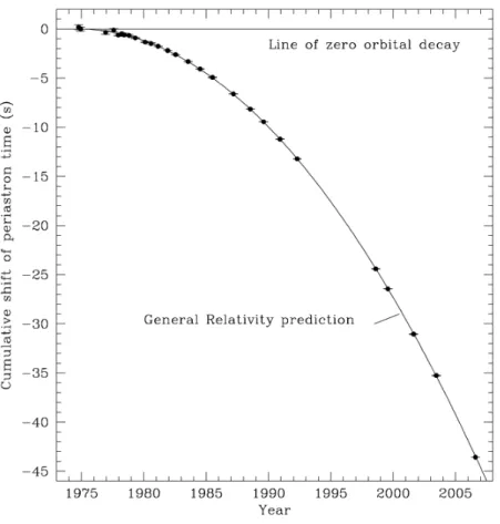
3.1 The orbital decay of the Hulse-Taylor binary pulsar. Radiative losses are computed using a leading order post-Newtonian approximation applied to Newtonian orbits, with results shown in Eqns. (3.65)-(3.67). Even in this approximate regime, observation has borne out the theory remarkably well. . . 33
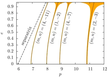
4.1 Orbital parameter space, resonances, and regions with near-static modes. Relativistic def-initions of semi-latus rectum p and eccentricity e are adopted [Eqn. (4.6)]. Dotted curves indicate, as in [8], a closed orbit with the ratio Ωϕ/Ωrbeing a rational number. On any such
curve there exists a static mode ωmn = mΩϕ+nΩr = 0 for indicated m and n. Within
the vicinity of these curves these modes will be nearly static. For near-static modes with frequencies below |ω| <10−4M−1 (shaded region) we use 128-bit floating point arithmetic
for part of the mode calculation. Our calculations are extended to frequencies as small as |ω|<10−6M−1, which exist in regions narrower than the dotted curves. . . . . 36
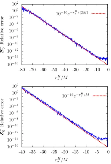
4.2 Subdominance instability and growth of roundoff errors with starting location. We demon-strate the effects of a subdominance instability by comparing results of numerical integrations begun at different initial radii rH
∗ near the horizon and ending at r∗ = 10M. The chosen
modes havel= 2 andM ω= 1 (odd parity on the left; even parity on the right). The fiducial, accurate solution is obtained from a high-order Taylor expansion, with sufficient terms that residuals are at or below roundoff even at a radius ofrH
∗ = 0. Using the Taylor expansion at
any −6M < rH
∗ <0 to begin an integration that then ends at r∗ = 10M gives results that
are consistent with each other. However, as smaller initial radii are chosen (rH
∗ <−10M),
exponentially greater errors are found in comparing atr∗= 10M the integrated mode and the fiducial Taylor expansion. We avoid the instability by beginning all integrations atrH
∗ =−6M
with initial conditions from the high-order Taylor expansion. . . 58 4.3 Semi-condition number growth of outgoing homogeneous solutions and effect of thin-QR
pre-conditioning. The left panel uses the even-parity mode (l, ω) = (5,5×10⁻³M−1) and plots as
a function ofr∗the semi-condition numberρof the matrixV, which is comprised of (the outer
solution) half of the Wronskian matrix. Two initial conditions are compared: the simple basis in red (dotted) and the thin-QR pre-conditioned basis in blue (solid). Orthogonalization with the thin-QR pre-conditioner makes a more than five orders of magnitude improvement. The right panel uses anl= 16 even-parity mode and shows the growth ofρin solutions that start with thin-QR orthogonalized initial conditions, as functions of frequency. Once the frequency reaches|ωM| ≤10−4, thin-QR pre-conditioning is no longer sufficient to control the condition
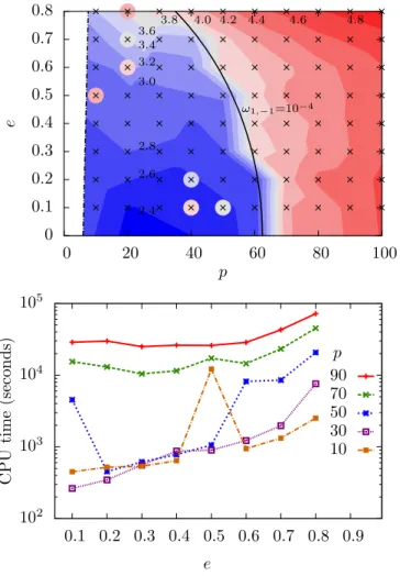
4.4 Plots of CPU time for GSF calculations as a function of orbital parameter space location. In the left panel labels give the log10 of CPU time in seconds for each contour. The crosses
indicate where models were computed. Every orbit on the right of the solid curve utilizes quad precision. Some orbits on the left lie near resonances, as indicated by local peaks in the contour plot caused by quad precision computing. Slices of CPU time versuse are shown in the right panel. GSF models require single-processor CPU times that range from 4 minutes to 1 day. . . 65 4.5 Contours of relative errors in the GSF. A grid of orbital parameters is chosen (crosses) and
the GSF is calculated. Resulting relative errors are used to generate contour levels of relative accuracy. Numerical labels indicate the log10of the relative error of each contour. . . 79
5.1 Equally spaced inχsampling ofp= 50,e= 0.7 orbit. The complete orbit is split intoN = 42 samples (∆χ= 0.1496) and spectral integration requires only N = 22 points betweenχ= 0 andχ =π(inclusive) to achieve double precision accuracy. The values ofdtp/dχ need only
be calculated at the indicated points to provide double precision integration and interpolation anywhere on the orbit. . . 90 5.2 Number of sample pointsN betweenχ= 0 andχ=πneeded to representdtp/dχ=g(χ) to
a prescribed accuracy. The ratio of magnitudes of the smallest to largest Fourier coefficients of g(χ) gives an estimate of the relative accuracy. The linear scaling of N versus digits of accuracy indicates geometric fall-off in the spectral components of g(χ). Away from the separatrix this relation is largely independent ofp. . . 91 5.3 Number of sample pointsN betweenχ= 0 andχ=πneeded to representdtp/dχ=g(χ) as a
function of eccentricityeat fixed accuracy of 150 decimal places. Of course as the eccentricity approaches unity and the radial period becomes infinite, so too does the number of needed samples. Still, for any astrophysically relevant orbit, we can sample the orbit to impressive accuracy with a modest number of points. . . 92 5.4 Aliasing effect from oversampling SSI in the FD. Shown here are energy flux data from an
orbit withp= 1020ande= 0.01 for modes withl= 2,m= 2. The energy flux from successive
nmodes falls off exponentially when computed away from the peak harmonic. Note that one harmonic (n=−m=−2) is nearly static, which decreases its flux by more than 100 orders of magnitude. As higher positive and negativenare computed, the fluxes reach Nyquist-like notches and oversampling innbeyond those points leads to increases in flux similar to aliasing. The locations of the minima scale with but are not equal to±N/2. . . 97 5.5 SSI at high accuracy. Absolute differences (errors) are shown in self-convergence tests. The
same data found in Fig. 5.4 are used to compute differences (per harmonic) in the fluxes between the three lower resolutions and the highest (N = 100) resolution. For each of the three lower resolutions (N = 40,60,80) the errors are well bounded by the accuracy criteria set by errors at the Nyquist notches. . . 98 5.6 Comparison between SSI withχsampling andtsampling as a function ofN and eccentricity.
The two sampling schemes are tested by examining convergence of thel = 2, m = 2, n= 0 energy flux using the MST code. All orbits havep= 103. . . 100
6.1 Enhancement function ϕ(et) associated with the 1.5PN tail. On the left the enhancement
function is directly plotted, demonstrating the singular behavior as et → 1. On the right,
the eccentricity singular factor (1−e2
t)−5 is removed to reveal convergence in the remaining
expansion to a finite value of approximately 13.5586 atet= 1. . . 128
6.2 The 3PN enhancement functionχ(et). Its log is plotted on the left. On the right we remove
the dominant singular factor−(1−e2
t)−13/2log(1−e2t). The turnover near et = 1 reflects
competition with the next-most-singular factor, (1−e2
t)−13/2. . . 130
6.3 The enhancement factorψ(et). On the right we remove the singular factor (1−e2t)−6and see
the remaining contribution smoothly approach a finite value atet= 1. . . 130
6.4 Fourier-harmonic energy-flux spectra from an orbit with semi-latus rectum p = 1020 and
eccentricity e= 0.1. Each inverted-V spectrum represents flux contributions of modes with various harmonic number n but fixed l and m. The tallest spectrum traces the harmonics of the l = 2, m = 2 quadrupole mode, the dominant contributor to the flux. Spectra of successively higher multipoles (octupole, hexadecapole, etc) each drop 20 orders of magnitude in strength aslincreases by one (l≤12 are shown). Every flux contribution is computed that is within 200 decimal places of the peak of the quadrupole spectrum. Withe = 0.1, there were 7,418 significant modes that had to be computed (and are shown above). . . 139 6.5 Residuals after subtracting from the numerical data successive PN contributions. Residuals
are shown for a set of orbits withp= 1020and a range of eccentricities frome= 0.005 through
e= 0.1 in steps of 0.005. Residuals are scaled relative to the Peters-Mathews flux (uppermost points at unit level). The next set of points (blue) shows residuals after subtracting the Peters-Mathews enhancement from BHP data. Residuals drop uniformly by 20 order of magnitude, consistent with 1PN corrections in the data. The next (red) points result from subtracting the 1PN term, giving residuals at the 1.5PN level. Successive subtraction of known PN terms is made, reaching final residuals at 70 orders of magnitude below the total flux and indicating the presence of 3.5PN contributions in the numerical fluxes. . . 139 6.6 Agreement between numerical flux data and the 7PN expansion at smaller radius and larger
eccentricities. An orbit with separation ofp= 103was used. The left panel shows the energy
flux as a function of eccentricity normalized to the circular-orbit limit (i.e., the curve closely resembles the Peters-Mathews enhancement function). The red curve shows the 7PN fit to this data. On the right, we subtract the fit (through 6PN order) from the energy flux data points. The residuals have dropped by 14 orders of magnitude. The residuals are then shown to still be well fit by the remaining 6.5PN and 7PN parts of the model even fore= 0.6 . . . 147 6.7 ”Strong-field comparison between the 7PN expansion and energy fluxes computed with a
LIST OF CONVENTIONS AND ABBREVIATIONS
Unless otherwise stated:
Metric signature (−,+,+,+)
Latin indicesi, j, k, l, . . . run over three spatial indices (1,2,3, orx, y, z)
Greek indicesα, β, γ, δ, . . . run over four spacetime coordinates (0,1,2,3 ort, x, y, z)
Units are geometrized c=G= 1
GR General Theory of Relativity
EM Electromagnetism
PE Principle of Equivalence
PGC Principle of General Covariance
GW Gravitational wave(s)
GSF Gravitational self-force
BHP Black hole perturbation
PN Post-Newtonian
PM Post-Minkowskian
EOM Equation(s) of motion
EMRI Extreme-mass-ratio inspiral
IMRI Intermediate-mass-ratio inspiral
CHAPTER 1: Introduction Section 1.1: Gravity as spacetime curvature
We begin by attempting to motivate Einstein’s insight that the appropriate relativistic treatment of gravity is a theory of curved four-dimensional spacetime, and we briefly sketch some of the fundamental mathematics. By necessity, we omit a vast amount of important detail, and refer the reader to any number of textbooks for more information. Much of this introduction closely follows [177] and [225].
Einstein’s key insight in formulating his general theory of relativity was the Principle of Equivalence (PE), which essentially states that the effects of an external gravitational field are indistinguishable from the effects of acceleration in a non-inertial frame of reference. In a freely-falling elevator, observers and test bodies experience the same acceleration due to an outside gravitational field, so the field appears to be “canceled” by inertial forces. Of course, this cancellation does not happen exactly if the field is inhomogeneous or time-dependent, but the cancellation can still be achieved if we restrict ourselves to a small region of space and time across which the field changes only negligibly. Therefore, Weinberg states the PE as follows [225]: “at every space-time point in an arbitrary gravitational field it is possible to choose a ‘locally inertial coordinate system’ such that, within a sufficiently small region of the point in question, the laws of nature take the same form as in unaccelerated Cartesian coordinate systems in the absence of gravitation.”
This particular statement of the PE is profoundly suggestive of the vital role that non-Euclidean geometry is to play in Einstein’s theory; just as physics is locally inertial (that is, well-described by special relativity), Riemannian manifolds are locally flat. As it turns out, this analogy is more than just suggestive. It leads us to an important restatement of the PE, called the Principle of General Covariance (PGC) [225]: A physical equation holds in a general gravitational field if (1.) the equation holds in the absence of gravitation, and (2.) the form of the equation is preserved under general coordinate transformationsx→x0, i.e. the equation
is “generally covariant.” As we shall see, the local reduction of a curved spacetime to the flat Minkowski metric implies geodesic, or freely-falling, motion, thereby describing the effects of gravitational fields.
1.1.1: Mathematical preliminaries
field. The metric is symmetric on exchange of its indices, meaning that it generally has ten algebraically independent components. It acts on infinitesimal coordinate displacements dxα to produce an invariant
spacetime interval,ds2:
ds2=g
αβdxαdxβ. (1.1)
Under a change of coordinatesxα=fα(x0µ
), the metric changes according to:
g0µν =gαβ
∂fα
∂x0µ
∂fβ
∂x0ν, (1.2)
butds2=g0 µνdx0
µ
dx0νremains unchanged. The coordinate transformations considered here are not required to be linear, and the coordinates may be general.
The metric also defines an inner product between vectorsAα andBβ,g
αβAαBβ, and is used to raise or
lower indices on vectors and tensors; given the vectorAα, its dualAα, a covector, is
Aα≡gαβAβ. (1.3)
Because coordinate lines are allowed to be arbitrarily curved, we need to generalize our notion of differentia-tion to allow for variadifferentia-tion in the underlying coordinate basis vectors (note that we encounter the same issue in flat space when using curvilinear coordinates). We define thecovariant derivative on a vector via
∇βAµ≡∂βAµ+ ΓµαβAα. (1.4)
Here,∂βis the usual partial derivative, and Γµαβ, theChristoffel symbols(or connection), encode information
about how the basis vectors change. They are computed from the metric,
Γµαβ=1 2g
µν(∂
αgνβ+∂βgνα−∂νgαβ). (1.5)
Covariant differentiation of a covector gives:
∇βAµ=∂βAµ−ΓαµβAα, (1.6)
and the covariant derivative of rank 2 tensors goes as:
∇βAµν =∂βAµν+ ΓµαβAαν+ ΓναβAµα, (1.7)
and the generalization to tensors of arbitrary rank is trivial.
Importantly, we choose the connection such that the the covariant derivative of the metric vanishes,
∇γgαβ=∇γgαβ= 0, (1.9)
implying, among other things, that the operations of index raising/lowering and covariant differentiation commute with one another.
1.1.2: Parallel transport and geodesic motion
Consider a timelike world line xα=rα(τ) parametrized by proper time τ, wheredτ =c−1√
−ds2. The
tangent vector to this worldline isuα=drα/dτ. We now define the derivative of a vector fieldAµ (defined
in some neighborhood around the world line) along the world line via
DAµ
dτ =u
β
∇βAµ. (1.10)
A vector is said to beparallel-transported along a world line when
DAµ
dτ = 0, (parallel transport), (1.11)
and a timelike world line rα(τ) is a geodesic of the spacetime when its own tangent vector uα is
parallel-transported along rα(τ). Intuitively, geodesics are the “straightest lines” of the geometry (examples are
great circles on the globe). By expanding the covariant derivative of Eqn. (1.10), we arrive at the geodesic equation
duµ
dτ + Γ
µ αβu
αuβ= 0, (1.12)
or
d2rµ
dτ2 + Γ µ αβ
drα
dτ drβ
dτ = 0. (1.13)
Again, we’ve made achoice here to use the metric-compatible connection for which Eqn. (1.9) holds. In a locally flat region of spacetime in which the Christoffel symbols can be taken to vanish, Eqn. (1.12) reduces to the statement duµ/dτ = 0. The acceleration vanishes, and the identity between freely-falling
We note that photons move on null geodesics of the spacetime, so that
drα
dλ drα
dλ = 0. (1.14)
1.1.3: Spacetime curvature and the Riemann tensor TheRiemann curvature tensor
Rαβγδ=∂γΓαβδ−∂δΓαβγ+ ΓαµγΓ µ βδ−Γ
α µδΓ
µ
βγ (1.15)
encodes information about the curvature of the spacetime, and, by virtue of a number of symmetries, has twenty algebraically independent components. It satisfies additionally a set of differential constraints known as theBianchi identities,
∇αRµνβγ+∇γRµναβ+∇βRµνγα= 0, (1.16)
to which we shall return later on.
The geometric content of the Riemann tensor is easily understood in terms of the geodesic deviation, which refers to the tendency of neighboring geodesics to approach or recede from one another. Consider a “congruence” of geodesicsxα=rα(τ, µ), where τ is a proper time andµa parameter which labels different
geodesics. Define the geodesic deviation vector ξ ≡ drα/dµ. Then, the equation of geodesic deviation is
given by
D2ξα
dτ2 =−R α
βγδuβξγuδ. (1.17)
This is a statement of relative acceleration between two geodesics in a curved spacetime, the presence of curvature therefore being indicated by the non-vanishing of the Riemann tensor. In a flat geometry, parallel (straight line) geodesics never cross, and their distance from one another remains constant. In its application to the theory of gravitational fields, Eqn. (1.17) is a statement about the effects of tidal forces on neighboring, freely-falling observers.
We may now define two more objects, the Ricci and Einstein tensors:
Rαβ≡Rµαµβ, (1.18)
Gαβ≡Rαβ−
1
whereR≡Rµ
µ=gαβRαβ. The Bianchi identities now lead to the “contracted Bianchi identities,”
∇βGαβ= 0. (1.20)
Finally, we make a note about the laws of physics in flat spacetime and their generalization to curved spacetime. The translation is remarkably simple. Starting with any physical equation, we rewrite it in tensorial form, in such a way that it is invariant under arbitrary Lorentz transformations. We then replace the flat space Minkowski metricηαβ with the appropriate curved space metric gαβ, and replace all partial
derivatives with covariant derivatives. The PE guarantees that the special relativistic physics is valid in any locally inertial frame, and hence justifies this prescription.
1.1.4: Einstein field equations
The Einstein field equations connect spacetime curvature, via the Einstein tensor defined in Eqn. (1.19), with the distribution of matter and energy in spacetime, via the stress-energy tensor,
Gµν = 8πTµν. (1.21)
Satisfaction of the Bianchi identities, Eqn. (1.20), implies that only six of the ten equations are truly inde-pendent. Recall that, in general, there are ten independent metric components. As we shall see, the field equations are not underdetermined; imposition of a gauge condition (equivalent to a choice of coordinates) provides another four constraints, bringing the number of independent metric components in line with the number of field equations.
Together, the field equations and the Bianchi identities imply
∇βTαβ= 0, (1.22)
which states that the stress-energy tensor must have vanishing divergence. In the special relativistic limit this amounts to local energy-momentum conservation.
These complications do not arise in electromagnetic theory, since electromagnetic fields are not themselves charged.
1.1.5: The Schwarzschild black hole solution
Because of the nonlinearity of the field equations, only a handful of exact, analytic spacetime solutions are known in GR. The results presented in this document have to do with motion in one of these spacetimes, called theSchwarzschild black hole solution. The Schwarzschild solution was the first nontrivial exact solution put forth after Einstein’s publication of the theory, though the implications of the singularities of this metric– a “true” singularity at the center of the black hole and a coordinate singularity at the horizon–were not fully understood for some years after Schwarzschild’s initial publication. It describes the static, spherically-symmetric vacuum spacetime in the vicinity of a non-rotating black hole. Here, we briefly motivate this solution.
We begin by proposing the most general form a static, isotropic spacetime metric,
ds2=B(r)dt2+A(r)dr2+r2dθ2+r2sin2θdφ2. (1.23)
The vacuum field equations read,
Rµν= 0. (1.24)
Eqn. (1.23) may be used to find the components of the Ricci tensor, and from (1.24) we find three nontrivial equations,
4A0B2−2rB00AB+rA0B0B+rB02A= 0, (1.25) rA0B+ 2A2B−2AB−rB0A= 0, (1.26) −2rB00AB+rA0B0B+rB02A−rB0AB= 0. (1.27)
Subtracting the first and third equations, we obtain
A0B+AB0= 0, (1.28)
implying that
whereK is a nonzero constant. Substitution of (1.29) into the middle equation gives
rA0 =A(1−A), (1.30)
which is solved by
A(r) =
1 + 1 Sr
−1
, (1.31)
whereS is another nonzero constant. Thus, the metric is now written
ds2=K
1 + 1 Sr
dt2+
1 + 1 Sr
−1
dr2+r2 dθ2+ sin2θdφ2. (1.32)
We are nearly done, but K and S are as yet undetermined. For these, one makes the physical argument that the geodesic equations of motion of this metric must reproduce the Newtonian equations of motion in the appropriate limit. It is shown that (in the geometrized units c =G= 1) K =−1, andS =−1/2M. Defining
f(r)≡1−rS
r, (1.33)
rS≡2M, (1.34)
whererSis the Schwarzschild radius, equal to twice the mass of the gravitational source (the black hole), we
have
ds2=−f(r)dt2+f(r)−1dr2+r2 dθ2+ sin2θdφ2. (1.35)
Section 1.2: The two-body problem in general relativity (GR)
The two-body problem is exceedingly simple to state: given the initial positions and velocities of two objects at some time t0, what are the positions and velocities of the objects at all future times t > t0? In
Newtonian gravity, it is not only simple to state, it is simple to solve. LetM ≡m1+m2 be the total mass.
Letting the origin of the coordinates be the location of the center of mass, definer≡r1−r2, wherer1 and
r2 are the position vectors form1 andm2, respectively. A few lines of manipulation then show that
¨
r=−GM
r2 ˆr. (1.36)
It is then straightforward to pose initial conditions and solve (1.36).
some sense, the two-body problem actually becomes athree-body problem in the context of GR; there are the two bodies as well as the gravitational field. The field has an associated energy, and so it acts as a gravitational field source itself.
In fact, what we are describing is the nonlinearity of the Einstein equations, which results in complicated self-interactions, e.g. gravitational waves (GWs) scattering off the background spacetime curvature. The effect of all of this is to greatly complicate the task of solving for the motion of the two masses.
Nevertheless, it is unacceptable not to make progress on the problem, not only because of its fundamental nature, but for its implications in predicting and analyzing gravitational wave signals using modern exper-iments. Gravitational waves, first predicted by Einstein in 1916 shortly after the publication of his general theory, are “ripples” in spacetime which propagate at the speed of light. The effects of a passing GW were long thought too small to measure, but indirect evidence for their existence was established with the obser-vation of the Hulse-Taylor binary pulsar PSR B1913+16 beginning in 1974, and GWs from the merger of a binary black hole system were directly detected by the LIGO collaboration in September 2015 [3]. We show how GWs arise mathematically in GR in Sec. 2, In the following section, we briefly describe the observational prospects for GWs from compact binary mergers.
Section 1.3: Gravitational radiation and observational interest
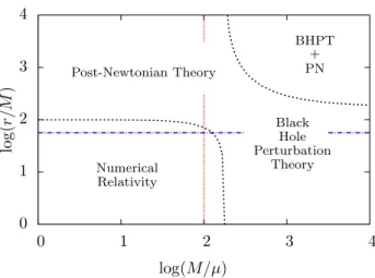
Merging compact binaries have long been thought to be a promising source of gravitational waves that may be found by ground-based or future space-based detectors. With the first observation of a binary black hole merger (GW150914) by Advanced LIGO [3], the era of gravitational wave astronomy has arrived. This first observation emphasizes what was long understood–that detection of weak signals and physical parameter estimation will be aided by accurate theoretical predictions. Both the native theoretical interest and the need to support detection efforts combine to motivate research in three complementary approaches [146] for computing merging binaries: numerical relativity [29, 148], post-Newtonian (PN) theory [226, 32], and gravitational self-force (GSF)/black hole perturbation (BHP) calculations [87, 20, 176, 207, 146]. Fig. 1.1 shows the regions of orbital parameter space for which these approaches are applicable. The effective-one-body (EOB) formalism then provides a synthesis, drawing calibration of its parameters from all three [49, 50, 64, 121, 65, 205].
0 1 2 3 4
0 1 2 3 4
log
(
r/
M
)
log(M/µ) Post-Newtonian Theory
Numerical Relativity
Black Hole Perturbation
Theory BHPT
+ PN
Figure 1.1: Regions of binary parameter space in which different formalisms apply. Post-Newtonian (PN) approximation applies best to binaries with wide orbital separation (or equivalently low frequency). Black hole perturbation (BHP) theory is relevant for binaries with small mass ratio µ/M. Numerical relativity (NR) works best for close binaries with comparable masses. The work presented in this document makes comparisons between PN and BHP results in their region of mutual overlap.
LIGO [48, 11]. Whether they exist, and have significant eccentricities, is an issue for observations to settle.
Section 1.4: Original contributions of this work and organization of document
As described in the previous section, there is strong astrophysical motivation for developing models of (highly) eccentric binary orbital dynamics for EMRIs and IMRIs. And yet to date, the bulk of the work in the field has been concerned with quasi-circular inspirals, for which the task is more straightforward. The original work presented in this thesis therefore aims to extend state-of-the-art, high-precision computational tools in BHP theory to the problem ofeccentricorbits on Schwarzschild black hole backgrounds. Further, we show how some of these BHP methods may be used toinformPN theory in its domain of common validity with BHP, and we present a set of original PN results along the way. This work constitutes a great leap forward in our understanding of and ability to accurately modeleccentric black hole mergers.
The document is organized as follows. We begin with introductions to the BHP and PN approximations, including discussion of the assumptions that underlie each formalism, and brief developments of the basic mathematical machinery in each case. We pay particular attention to the problem of gravitational radiation and binary systems.
Figure 1.2: The probability distribution function for a compact object entering the LISA passband as a function of orbital eccentricity according to the possible binary formation mechanism described in [123]. As the figure shows, it is likely that highly-eccentric orbits will be important sources for any LISA-like experiment. Figure taken from [123].
Ch. 5 describes what we’ve termed the method of spectral source integration (SSI), a formalism for evaluating integrals over the source terms in perturbation problems to remarkably high precision at modest computational cost. This work was also previously published, as Ref. [127].
The development of SSI was key in extending use of the Mano-Suzuki-Takasugi (MST) formalism to the eccentric orbit case. The MST method provides means for computing metric perturbations in a post-Newtonian regime to arbitrarily high precision using semi-analytic expansions. Ch. 6 describes an application of these new techniques, in which we leverage high-precision MST calculations to fit out and determine heretofore unknown, high-order parameters in the PN expansion for the energy flux for eccentric inspirals. The basis for this chapter was a third publication, listed here as Ref. [102].
CHAPTER 2: BHP and GSF: background and development Section 2.1: Assumptions and applicability
As mentioned in the Introduction, the GSF approach is relevant when the binary mass ratio is sufficiently small that the motion and field of the smaller mass can be treated in a perturbative expansion. In this black hole perturbation (BHP) theory, the background field is that of the heavier stationary black hole and the zeroth-order motion of the small mass is a geodesic in this background. Then the perturbation in the metric is calculated to first-order in the mass ratio and the action of the field of the small body back on its own motion is computed (i.e., the first-order GSF) [158, 185]. In principle the calculation proceeds to second-order [116, 181] and beyond. Over the past fifteen years a number of key formal developments have been established [158, 185, 24, 77, 117, 179].
Work on the GSF approach has been motivated in part by prospects of detecting extreme-mass-ratio inspirals (EMRIs) using a space-based gravitational wave detector like LISA or eLISA [9, 160, 89]. For a LISA-like detector withfmin'10−4Hz, an EMRI consists of a small compact object of massµ'1−10M
(neutron star or black hole) in orbit about a supermassive black hole (SMBH) of massM ∼105
−109M .
The mass ratio would lie in the rangeε=µ/M '10−9
−10−4, small enough to allow a gradual, adiabatic
inspiral and provide a natural application of perturbation theory. As the EMRI crosses the detector passband prior to merger its orbital motion accumulates a total change in phase of orderε−1∼104−109 radians.
Less extreme mass ratios may also be important. A class of intermediate mass black holes (IMBHs) may exist with masses M ∼ 102−104M
. These are suggested [156] by observations of ultraluminous X-ray
sources and by theoretical simulations of globular cluster dynamical evolution. Stellar mass black holes or neutron stars spiralling into IMBHs with masses M ∼50−350M, referred to as intermediate-mass-ratio inspirals (IMRIs), would lie in the passband of Advanced LIGO and are potentially promising sources [48, 11]. An IMRI might also result from binaries composed of an IMBH and a SMBH [11], which would appear as an eLISA source. While IMRIs execute fewer total orbits (i.e., ε−1
∼ 102
−103) than EMRIs in making,
say, a decade of frequency change, the theoretical approach is nearly the same. Detection of E/IMRIs would represent another strong field test of general relativity and measurement of the primary’s multipole structure would confirm or not the presence of a Kerr black hole [212, 22, 48].
The dominant approach to date takes the small body to be a point mass [176], computes the metric perturba-tion (MP) in the time domain (TD) [155, 25, 92, 52] or frequency domain (FD) [74, 126, 7], and obtains a finite self-force from the divergent retarded field by mode-sum regularization [24, 25, 74, 26, 27, 19, 7, 221, 8]. Work on the gauge dependent GSF has benefited from analogous scalar field models [75, 118, 18]. Applications to Kerr EMRIs, both with scalar and gravitational self-force, have been made [16, 215, 141, 82, 195, 85, 128, 214]. Availability of analytic mode-sum regularization parameters [119, 120] has been beneficial. Calculations of perturbations and the GSF have now been made with very high accuracy, arbitrary precision arith-metic [103, 196, 198, 102], allowing detailed comparison with PN theory (see also [74, 34]). Indeed, these comparisons form an important part of the original work in this thesis (see Secs. 6 and 7). Finally, alter-native means of calculating the self-force, both effective source calculations [210, 211, 223] and direct Green function calculations [53, 54, 222], are being developed.
Section 2.2: Linearized field equations in flat spacetime
We first review how the Einstein equations are linearized about flat spacetime. Much of the development in this section follows [177]. Assume that the metric can be expressed in the form
gαβ=ηαβ+pαβ, (2.1)
whereηαβ is the flat space Minkowski metric – the “background” – andpαβ is a “small perturbation.” We
say thatpαβ =O(), with1. Eqn. (2.1) describes weakly-curved spacetime. Our plan is to insert this
expression into the Einstein field equations and expand, keeping terms only to linear order in.
The decomposition (2.1) puts restrictions on the general coordinate freedom that we have in GR. That is, we shall now allow only coordinate transformations which preserve the character of the metric as being “mostly Minkowski.” We consider small coordinate transformations of the form
x0α=xα+ζα(xβ), (2.2)
where ζα =
O(). It is straightforward to show that under these conditions the metric perturbation then transforms as
p0αβ=pαβ−∂αζβ−∂βζα, (2.3)
where indices are raised or lowered using the backgroundηαβ, e.g. ζα≡ηαµζµ.
is simply a restricted representation of the full covariance of GR. Such infinitesimal coordinate freedom shows up at each order in perturbation theory. We also have the freedom in linearized gravity to change global Lorentz frames.
Now, the inverse perturbed metric is defined by
pαβ≡ηαµηβνpµν, (2.4)
and the trace of the metric perturbation is
p≡ηαβpαβ. (2.5)
(Note that tensor indices are being raised and lowered using the flat spacetime Minkowski metricηαβ.) To
linear order in, the inverse of the full metric is
gαβ=ηαβ
−pαβ. (2.6)
The Christoffel symbols and the Riemann tensor are now
Γαβγ =
1 2 ∂βp
α
γ+∂γpαβ−∂αpβγ, (2.7)
Rαβγδ=
1
2(∂βγpαδ−∂βδpαγ−∂αγpβδ+∂αδpβγ). (2.8) Here, we have introduced the notation∂αβ≡∂α∂β to denote the second derivative.
Note that the Riemann tensor is invariant under gauge transformations, R0
αβγδ = Rαβγδ, a statement
that its physical content (the spacetime curvature) does not depend on any choice of coordinates. We may now derive the linearized Ricci tensor and scalar, and the linearized Einstein tensor:
Rαβ=−1
2 pαβ+∂αβp−∂αµp
µ
β−∂βµpµα
, (2.9)
R=−p+∂µνpµν, (2.10)
Gαβ=−
1
2 pαβ+∂αβp−∂αµp
µ
β−∂βµpµα
+1
2ηαβ(p−∂µνp
µν). (2.11)
Here,≡ηµν∂
µν is the flat spacetime d’Alembertian (wave operator).
It turns out to be convenient, especially in the following sections, to introduce the “trace-reversed metric perturbation,”
¯
pαβ≡pαβ−1
which has the property, as its name implies, that ¯p = −p. One then finds pαβ = ¯pαβ− 12ηαβp, and on¯
substitution we obtain
Gαβ=−
1 2
¯pαβ−∂αµp¯µβ−∂βµp¯µα+ηαβ∂µνp¯µν
. (2.13)
The field equations still take the form
Gµν = 8πTµν, (2.14)
whereTµν must now also be taken, in some appropriate sense, to be of order. The Bianchi identities and
the condition of energy-momentum conservation at this order reduce to
∂βGαβ= 0, (2.15)
∂βTαβ= 0. (2.16)
2.2.1: Lorenz gauge
Until now, we have not yet invoked the freedom described by Eqn. (2.3); we’ve so far left the gauge unspecified. It turns out to be very convenient to adopt what is known asLorenz gauge, meaning we impose the four conditions
∂βp¯αβ= 0. (2.17)
This is a generalization of the identically named gauge condition in EM theory. It is always possible to transform the metric perturbation such that (2.17) is satisfied, and it can be shown that the generator ζα of the gauge transformation from some ¯poldαβ, which does not satisfy (2.17), to some ¯pnewαβ , which does
satisfy (2.17), obeys
ζα=∂βp¯oldαβ. (2.18)
However, the conditions (2.17) are not unique; to any gauge generator ζα satisfying (2.18), we may add
some ζhom
α which satisfiesζαhom= 0. For this reason, the Lorenz gauge is known as a “differential gauge.”
Note also that in this discussion, we are using “gauge” to refer to a condition on the metric perturbation, pαβ. This is distinct from the freedom we have to specify coordinates for the background metric; as we’ve
pointed out, gauge freedom arises at each order in a perturbative expansion like the one in Eqn. (2.1). In any case, the conditions (2.17) ensure that there are six independent metric perturbation components (ten by symmetry, minus another four).
conditions, we find that the Einstein tensor and the field equations take the convenient form
Gαβ=−
1
2¯pαβ, (2.19)
p¯αβ=−16πTαβ. (2.20)
As we shall see, of the six independent degrees of freedom ofpαβ, two are radiative, and the remaining four
are tied to the distribution of matter.
2.2.2: The plane wave solution and gravitational wave polarizations In the following, we take cues from [93]. In a vacuum, we have
¯pµν = 0, (2.21)
∂νp¯µν = 0. (2.22)
By considering only homogeneous, asymptotically flat solutions to the linearized field equations (2.21), it is possible, having specified Lorenz gauge, to further specialize the gauge, using the residual gauge freedom, such that the metric perturbation is purely spatial,
ptt=pti= 0, (2.23)
as well as traceless
p≡pii= 0. (2.24)
In this case, the Lorenz gauge condition ensures that the spatial metric perturbation is transverse,
∂ipij= 0, (2.25)
and so this more specific gauge is known astransverse-tracelessgauge, or TT gauge. Note that in TT gauge, the distinction between ¯pij andpij is unimportant. Also, note that in (2.25) we may as well have written∂i,
since the position of spatial indices in Cartesian coordinates is irrelevant, but we wanted to be clear about the implied summation.
When the TT gauge conditions are imposed, there is no longer any residual gauge freedom; the gauge is completely specified. Furthermore, the metric perturbation pTT
ij now contains only physical, non-gauge
There is now a nice relationship between the linearized Riemann tensor and the metric perturbation,
Ritjt=−
1 2p¨
TT
ij . (2.26)
In a globally vacuum spacetime, all nonvanishing components of the Riemann tensor can be obtained from Ritjt by symmetries of the tensor and the Bianchi identities. In a more general spacetime, the Riemann
tensor will have components which are not related to radiation, but tied to the matter distribution.
Another advantage of TT gauge is that it makes clear that there are only two radiative degrees of freedom, corresponding to two gravitational wave polarization states. Consider a wave propagating along the +z-axis,
pTTij =pTTij (t−z). (2.27)
The Lorenz gauge condition implies thatpTTzj must be a constant. In particular, the condition thatpij→0
as r→ ∞requires that this constant be zero. The only nonzero components are thenpTT
xx, pTTxy, pTTyx, and
pTT
yy, but symmetry and the trace-free condition guarantee that only two of these are independent. We define
pTTxx =−pTTyy ≡p+(t−z), (2.28)
pTTxy =pTTyx ≡p×(t−z), (2.29)
to be the two plane wave polarizations.
Section 2.3: Perturbations on curved spacetimes
In the previous sections, we linearized the Einstein equations around the flat spacetime (Minkowski) metric,ηµν, and saw that Eqn. (2.20) governed the resulting perturbation. We could instead set about
lin-earizing the field equations around an arbitrarily curved background metricgµν. By analogy with Eqn. (2.1),
we say that the full spacetime metric may be written
gµν =gµν+pµν+O(2), (2.30)
where, once again, pµν is a “small” perturbation of O(). Inserting (2.30) into (1.21) and dropping terms
which are quadratic or higher inpµν, we find [23]
where a stroke |µ (or ∇µ) indicates covariant differentiation with respect to the background metric gµν,
indices are raised or lowered using the backgroundgµν, and≡|λ|λ is the curved spacetime d’Alembertian
operator. As before,p≡gµνpµν is the trace of the metric perturbation.
Introducing once again the trace-reversed metric perturbation
¯
pαβ≡pαβ−
1
2gαβp, (2.32)
and imposing the Lorenz gauge conditions, which now read
¯
pαβ|β= 0, (2.33)
Eqn. (2.31) becomes
¯pαβ+ 2Rµανβp¯µν =−16πTαβ (2.34)
Notice the similarity of this result with Eqn. (2.20); the difference here is the Riemann term coupling the perturbation with the background curvature.
Eqn. (2.34) is a system of ten linear, second-order, hyperbolic equations, which admits a well-posed initial value formulation on a spacelike Cauchy hypersurface. A substantial portion of the original work presented in this thesis is devoted to a high-precision, frequency domain algorithm for solving (2.34) in the context of EMRIs on Schwarzschild backgrounds, where the perturbation is induced by the motion of a small compact object (modeled as a structureless point particle) whose trajectory is a bound, eccentric geodesic of the background geometry. The reader is referred to Sec. 4 for details.
Section 2.4: Self-force
In both electromagnetism and gravitation, radiation results in a local backreaction which perturbs the motion of the radiating body. These effects can be thought of as arising from an interaction of the body with its own field, or aself-force (SF).
2.4.1: Newtonian self-force
Though rarely encountered (or at least, discussed in these terms) in elementary courses on Newtonian mechanics, the SF is not just a relativistic effect. Consider solar system orbits. Typically, we think of the Earth’s orbit about the Sun as being equivalent to free-fall in the Sun’s gravitational field. For circular motion, Newton’s second law would say
ma= GMm
r2 , (2.35)
lettingmbe the mass of the Earth, or any other body in orbit about the sun at orbital radiusr. The orbital period is then
T = 2π
s
r3
GM. (2.36)
To be more accurate, we must also include the influence of the Earth on the Sun; the Earth is in free-fall in the Sun’s field, while the Sun is in orbit about the common center of mass. The result in this case is
T = 2π
s
r3
GM
1 + m M
. (2.37)
Perhaps it is more appropriate to say that the change here is not so much due to an interaction of the Earth with its own field, but due instead to the fact that the Sun’s own orbit has been perturbed. This is suggestive of another interpretation of the SF when we move to GR; we can think of the motion of a small orbiting body as “forced” motion on the background spacetime of the larger object, or we can think of the motion as being geodesic in a perturbed spacetime. Either view is valid mathematically, but there are conceptual advantages to the latter.
2.4.2: Electromagnetic radiation-reaction/self-force
Dirac, among others, provided a derivation of the electromagnetic radiation-reaction force experienced by a radiating electron [80], which we summarize here.
Recall the electromagnetic four-potential Aµ, satisfying
∂µAµ= 0, (2.38)
Aµ= 4πjµ, (2.39)
wherejµ is the charge-current density. The electromagnetic tensorFµν is then given by
In this section, indices are raised or lowered using the flat spacetime Minkowski metricηµν.
For a single electron, the current vector is zero everywhere, and infinite along the worldline, zµ(s),
jµ=e
Z dz
µ
ds δ(x0−z0(s))δ(x1−z1(s))δ(x2−z2(s))δ(x3−z3(s))ds. (2.41)
Of course, Eqns. (2.38) admit many solutions, and in particular we may take linear combinations of solutions, or add to an existing solution anotherAµ obeying∂
µAµ= 0 andAµ= 0.
The physically interesting solution is the retarded solution for fields emitted by the electron, the Li´enard-Wiechert potential Fret
µν. However, there is a corresponding advanced solution, physically representing
in-coming fields absorbed by the charge,Fadv
µν . Dirac showed that the singular part of the field (that part which
diverges at the location of the electron) is given by the mean of these retarded and advanced parts,
FµνS =
1 2 F
ret µν +Fµνadv
. (2.42)
Detweiler notes that here the “S” might also stand for “symmetric,” given the clear causal symmetry of (2.42). Though this solution is causally unphysical, it is a valid solution to the sourced Maxwell’s equations.
Dirac then shows that this field exerts no net force on the electron in the limit that the charge q→0. We then define the remainder, orregular field
FµνR ≡Fµνret−FµνS =
1 2 F
ret µν −Fµνadv
. (2.43)
It is then shown that this regular field is responsible for the radiation-reaction force,
Frad
β =quαFαβR, (2.44)
atxα=zα(s). This force is more commonly expanded and rewritten as
Frad =
2 3
q2
c3v,¨ (2.45)
This is related to the charge’s dipole moment; it is a dipole radiation effect. Note that Fret
µν and FµνS are both solutions to Maxwell’s equations with identical sources, and therefore
FR
µν is a vacuum solution. That is, locally the regular field is source-free and its origin apparently cannot be
2.4.3: Gravitational radiation-reaction/self-force
We now turn attention to the gravitational self-force problem, for which we shall draw many parallels to the electromagnetic case just described. To begin with, consider the perturbative split defined in Eqn. (2.30); starting with a background geometrygµν, we seek an approximate solution gµν+pretµν to the Einstein field
equations, or, schematically,
G(g+pret) = 8πT+O(p2). (2.46)
Here, the perturbation is thought to arise from the motion of some small massm, which at zeroth order in this scheme moves along a geodesic ofgµν.
We now define the regular fieldpR µν via
pretµν =pSµν+pRµν. (2.47)
This is known as the Detweiler-Whiting decomposition [77]. It can then be shown that, at this order of approximation,mmoves along a geodesic not ofgµν, but ofgµν+pRµν.
We may go further: the purelydissipative part of the field is given by
pdissµν =
1 2 p
ret µν−padvµν
, (2.48)
whereas the conservative parts of the field are given by
pconµν =pRµν−pdissµν
=1 2 p
ret µν +padvµν
−pSµν. (2.49)
Clearly,
pR
µν =pconµν +pdissµν . (2.50)
Though we’ve expressed some preference for thinking of the radiation-reaction effect as being geodesic motion in a perturbed background, there does indeed arise a force on the particle when viewed from an initial background geodesic. From this point of view, the resulting acceleration off the background worldline is
uβ∇βuα=− gαβ+uαuβuγuδ
∇γpRδβ−
1 2∇βp
R γδ
. (2.51)
CHAPTER 3: PN theory: background and development Section 3.1: Assumptions and applicability
The post-Newtonian approximation has a rich history, dating back to just after Einstein’s first publication of the full theory, when Einstein himself developed the quadrupole moment wave generation formalism [88], later refined by Landau and Lifshitz [145]. Even after nearly a century of effort, the current state-of-the-art for the PN equations of motion (EOM) is 4PN (i.e. fourth-order in a PN expansion). The 1PN EOM were obtained by Lorentz and Droste [149], Einstein, Infeld, and Hoffman [2], and Fock [95]. At 2PN order, the EOM were worked out by Ohta, Okamura, Kimura, and Hiida [164, 166, 165], and the 2.5PN EOM were determined by Damour and Deruelle [63, 67, 66, 62] and Itoh, Futamase, and Asada[129]. Non-conservative–ordissipative–effects, related to the emission of gravitational radiation, enter the approximation at 2.5PN. The 3PN EOM were derived by Jaranowski, Sch¨afer, and Damour [133, 134, 132, 68, 69], by Blanchet and Faye [42, 41, 43, 44], by Futamase and Itoh [106], and by Foffa and Sturani [97]. To obtain the 3.5PN EOM, the 1PN correction to the radiation-reaction force is needed. These were obtained by Iyer and Will [130, 131] for point-mass binaries. The 2PN correction was then obtained by Gopakumar, Iyer, and Iyer [113]. Gravitational wave tail effects arise at 4PN order, and modify the radiation damping force as a 1.5PN correction [33, 98, 107]. Partial progress was made on the 4PN EOM by Jaranowski and Sch¨afer [135, 136, 137] and by Foffa and Sturani [96], with the complete dynamics being worked out by Damour, Jaranowski, and Sch¨afer [70]. Work done by Bini, Damour, and Geralico [31], as well as work by Hopper, Kavanagh, and Ottewill [125], have confirmed these results in the test body limit.
instantaneous (non-tail) contributions from relativistic corrections to the source moments, which have been developed by Blanchet, Iyer, Joguet, and Faye [36, 46, 45]. The extension of these results to the eccentric case was accomplished by Arun, Blanchet, Iyer, and Qusailah [14, 13, 15],
Comparisons between PN and BHP theory calculations were made by Poisson [173], Tagoshi and Naka-mura [201], and by Sasaki, Tagoshi, and Tanaka [194, 202, 204]. More recent work by Fujita [103] and Shah, Friedman, Whiting, and Johnson-McDaniel [196, 198, 139] made use of advances in BHP theory to compute PN corrections to extremely high order (up to 22PN). This work has been done primarily in the context of circular orbits. In 2015, Sago and Fujita [191] computed the rates of change of the orbital parameters under radiation reaction for eccentric orbits to 4PN order in the test mass limit.
In this chapter, we attempt to give a flavor for the PN approximation in GR, as well as the related, but “upstream” (i.e. more fundamental) post-Minkowskian (PM) expansion. We largely follow [177], [32], and [225] in our development of the following material.
When describing an approximation as being “post-Newtonian,” we sometimes interchangeably say that we are using a “slow-motion” assumption. However, we can be a bit more precise: the PN approximation is valid in the near-zone of a slowly-moving, weakly self-gravitating source. Given a source stress-energy tensor Tαβ and a source Newtonian potentialU, we define the small PN parameteras
≡max
( T
0i
T00 ,
T
ij
T00
1/2
,
cU2
1/2)
1. (3.1)
So again, where we might often say thatv/c1 in the PN regime, it is more accurate to refer to Eqn. (3.1). Note also that for this chapter, we temporarily depart from our unit convention which setsc=G= 1, since we use these constants as book-keeping parameters to keep track of the size of expansion terms.
![Figure 1.2: The probability distribution function for a compact object entering the LISA passband as a function of orbital eccentricity according to the possible binary formation mechanism described in [123].](https://thumb-us.123doks.com/thumbv2/123dok_us/8255480.2187239/27.918.258.660.110.429/probability-distribution-function-eccentricity-according-formation-mechanism-described.webp)