Gidcumb_unc_0153D_14825.pdf

(1)

PERFORMANCE OF A CARBON NANOTUBE FIELD EMISSION X-RAY SOURCE ARRAY FOR STATIONARY DIGITAL BREAST TOMOSYNTHESIS

Emily Morgan Gidcumb

A dissertation submitted to the faculty at the University of North Carolina at Chapel Hill in partial fulfillment of the requirements for the degree of Doctor of Philosophy in the

Department of Applied Physical Sciences (Materials Science).

Chapel Hill 2014

Approved by: Otto Zhou

Alfred Kleinhammes Yueh Z. Lee

(2)

(3)

ABSTRACT

Emily Morgan Gidcumb: Performance of a carbon nanotube field emission X-ray source array for stationary digital breast tomosynthesis

(Under the direction of Otto Zhou and Jianping Lu)

This work describes the performance of a stationary digital breast tomosynthesis (s-DBT) X-ray tube based on carbon nanotube (CNT) cathodes, and the imaging system developed around it. The s-DBT system has the potential to improve the detection and diagnosis of breast cancer over commercially available digital breast tomosynthesis (DBT) systems. DBT is growing in popularity in the United States, and around the world, as a potential replacement for traditional 2D mammography. The main advantage of DBT over 2D mammography lies in the pseudo-3D nature of the technique allowing the removal of overlapping breast tissue within the image. s-DBT builds on this advantage by removing blur from focal spot motion.

Introductions to breast imaging techniques and the DBT modality are given, followed by an introduction to carbon nanotube field emission, the foundation of the s-DBT

technology. Details of the s-DBT X-ray tube design and system integration are discussed including specific design parameters, system requirements, and the development process. Also included are summaries of the X-ray tube and system performance over time, and results from characterization measurements.

(4)

spatial resolution with use of the focusing electrodes. The tungsten gate mesh is an essential component for extracting electrons from CNTs. A successful deep reactive ion etching fabrication procedure was developed, and the improved gate mesh allowed for higher cathode current and longer pulse widths to be employed in the s-DBT system.

Characterization of the CNT cathodes revealed their high-current capacity and the ability to produce relatively long pulse widths, mimicking a 2D imaging modality. This work

confirmed that the cathodes are well suited for the task of breast imaging, and explored possible improvements. Lastly, it was shown that by employing and optimizing the focusing electrodes, spatial resolution of the s-DBT system improved, with a tradeoff in loss of

(5)

Let the words of my mouth and the meditation of my heart be acceptable in your sight, O Lord, my rock and my redeemer.

(6)

ACKNOWLEDGEMENTS

This research was funded through the National Cancer Institute (R01-CA134598) and the Carolina Center of Cancer Nanotechnology Excellence, also funded by the National Cancer Institute, through grant U54-CA151652.

I would first like to thank my advisors, Dr. Otto Zhou and Dr. Jianping Lu. Dr. Zhou, you have been amazing in guiding and redirecting me over the years. The support and understanding you have shown have been invaluable to me. I truly would not have been able to participate in this great work without you. Dr. Lu, I really appreciate your patience and help with my questions over the years, and your advice on the direction and content of my work. It was a pleasure working with you.

(7)

Thank you to all those who helped in the editing and proofreading of this thesis: Lance Gidcumb, Sean Washburn, Allison Hartman, and Shaun Gidcumb.

I would like to acknowledge Dr. Bo Gao and Ai Leen Koh for their collaborations on published works. It was a joy working with both of you. Also, I give a big thank you to Derrek Spronk for all your practical help and assistance over the years. I always appreciated your willingness to help.

Thanks to all of my lab members, past and present. Xiomara Calderòn-Colòn and Shabana Sultana, we did not work together long but I treasured that time and value the relationships we have continued since. Xin Qian, you taught me so much when I started in the lab. Christy Inscoe, there is not enough space to list all of the ways you have been a help to me, in addition to the help you gave me in my research. I do not believe I would have gotten to this point had you not been a part of my life. Lei Zhang, I’m so lucky to have found one of my dearest friends in a lab mate. You have made this whole experience better in innumerous ways. I would like to specially thank those who worked with me on the breast tomosynthesis project: Andrew Tucker and Jabari Calliste. It was a lot of work, but we had a lot of fun along the way, too. Jing Shan and Pavel Chtcheprov, I want to thank you both for help on various portions of my research over the years. Marci Potuzko, Allison Hartman, and Gongting Wu, thanks for making the lab more fun. It has been great getting to know and work with you all.

(8)

would also like to thank my brother, Andrew Morgan; my in-laws, Lance and Candy Gidcumb; my cousins, Anna Stout and Rand Allingham; and my grandparents, James and Jenny Case and Doris Morgan. I love you all more than words can say, and space would allow.

(9)

PREFACE

Portions of several chapters in this work have been previously published in other locations, with my participation as an author or co-author. All reused portions are noted, as they appear, throughout this work.

Chapter 5, titled “Initial Performance of CNT X-ray Source for Stationary Digital Breast Tomosynthesis”, contains text and figures from Qian, X. et al., “High resolution stationary digital breast tomosynthesis using distributed carbon nanotube x-ray source array”, Med. Phys., 39 (2012); as well as Gidcumb, E. et al., “Carbon nanotube electron field

emitters for X-ray imaging of human breast cancer”, Nanotechnology 25 (2014). Other portions of Gidcumb, E. et al., “Carbon nanotube electron field emitters for X-ray imaging of human breast cancer”, Nanotechnology 25 (2014) appear in Chapter 6, titled “Long Pulse Width Field Emission Testing of Cathodes”, and in Chapter 7, titled “s-DBT System Performance”. Chapter 6 also includes a portion of the work by Koh, A. L et al.,

“Observations of Carbon Nanotube Oxidation in an Aberration-Corrected Environmental Transmission Electron Microscope”, ACS Nano 7, 2566-2572 (2013). Furthermore, Chapter 7 includes work from Tucker, A. W. et al. in Medical Imaging 2013: Physics of Medical Imaging. (SPIE, 2013).

Other work in Chapter 7 has been reused, with permission, from Tucker, A. W., Lu, J. & Zhou, O. “Dependency of image quality on system configuration parameters in a

(10)

al. “Increased microcalcification visibility in lumpectomy specimens using a stationary

(11)

TABLE OF CONTENTS

LIST OF TABLES ... xviii

LIST OF FIGURES ... xxi

LIST OF ABBREVIATIONS AND SYMBOLS ... xxxi

CHAPTER 1: INTRODUCTION ... 1

1.1 Importance of breast imaging ... 1

1.2 Motivation for improving breast imaging ... 2

1.3 Mammography ... 3

1.3.1 Mammographic features ... 3

1.3.1.1 Masses ... 3

1.3.1.2 Calcifications ... 7

1.3.2 Non-radiographic imaging modalities used with mammography ... 9

1.3.2.1 Ultrasound ... 9

1.3.2.2 Magnetic resonance imaging ... 12

1.3.3 Current state of X-ray mammography ... 15

1.3.3.1 The physics of X-ray imaging ... 15

1.3.3.1.1 Electromagnetic radiation ... 15

1.3.3.1.2 Production of X-rays ... 16

(12)

1.3.3.1.4 X-ray attenuation ... 21

1.3.3.1.5 Absorption of X-ray energy ... 22

1.3.3.2 Technique ... 24

1.3.3.2.1 Equipment ... 24

1.3.3.2.2 Positioning ... 31

1.3.3.3 Goals, trends, and limitations ... 33

1.4 Digital breast tomosynthesis ... 36

1.4.1 Main principles ... 36

1.4.2 Technique and current systems ... 39

1.4.3 Advantages over FFDM ... 43

1.4.4 FDA approval... 47

1.5 REFERENCES ... 1

CHAPTER 2: MOTIVATIONS FOR AND FOUNDATIONS OF STATIONARY DIGITAL BREAST TOMOSYNTHESIS ... 3

2.1 Limitations of current DBT methods ... 3

2.2 Basic idea and proposed advantages of s-DBT... 6

2.3 Materials science of s-DBT ... 8

2.3.1 Theory of field emission ... 8

2.3.2 Field emission versus thermionic emission for X-ray production ... 10

2.3.3 CNT properties as field emitters ... 15

2.3.4 Altered CNTs and other materials for field emission ... 23

(13)

CHAPTER 3: DESIGN AND DEVELOPMENT OF THE STATIONARY DIGITAL BREAST TOMOSYNTHESIS SYSTEM ... 36

3.1 Tube design ... 36

3.1.1 Electrode structure ... 36

3.1.2 Tube layout and properties ... 42

3.2 System design and build challenges ... 48

3.2.1 Overall system information... 48

3.2.2 X-ray tube construction... 50

3.2.3 Tube and system evaluation ... 50

3.2.4 Electronic controls integration and system summary ... 52

3.2.5 Reconstructions ... 54

3.2.6 FDA requirements ... 54

3.3 Other CNT X-ray sources ... 55

CHAPTER 4: FABRICATION OF TUNGSTEN METAL GATE MESH... 60

4.1 Introduction ... 60

4.1.1 Various gate mesh used in CNT X-ray sources ... 60

4.1.2 Deep reactive ion etching... 63

4.1.3 Tungsten etching alternatives ... 65

4.2 Methods... 67

(14)

4.2.2 Complete procedure for tungsten gate mesh fabrication ... 68

4.3 Results ... 72

4.4 Discussion ... 76

4.5 Conclusion ... 78

CHAPTER 5: INITIAL PERFORMANCE OF CNT X-RAY SOURCE FOR STATIONARY DIGITAL BREAST TOMOSYNTHESIS ... 81

5.1 Argus 3.0 performance characterization ... 81

5.1.1 Anode heat capacity ... 81

5.1.2 Current characteristics of CNT cathodes ... 83

5.1.3 Focal spot sizes ... 86

5.1.4 Spatial resolution ... 87

5.1.5 Phantom imaging ... 89

5.2 Additional tomosynthesis accelerated lifetime tests ... 91

5.2.1 Motivation and methods ... 92

5.2.2 Results ... 93

5.2.3 Conclusions ... 97

CHAPTER 6: LONG PULSE WIDTH FIELD EMISSION TESTING OF CATHODES ... 100

6.1.1 Motivation ... 100

(15)

6.1.3 Differences in nanotube fabrication ... 103

6.1.3.1 FWNTs with thermal CVD ... 103

6.1.3.2 MWNTs with arc discharge ... 104

6.2 Methods... 104

6.3 Results ... 108

6.3.1 Initial I-V curves ... 108

6.3.2 FWNT results ... 110

6.3.2.1 4 s pulses ... 110

6.3.2.2 3 s pulses ... 113

6.3.2.3 2 s pulses ... 115

6.3.3 MWNT results ... 117

6.3.3.1 4 s pulses ... 117

6.3.3.2 3 s pulses ... 118

6.3.3.3 2 s pulses ... 119

6.3.4 SEM images of cathodes ... 122

6.3.4.1 FWNT cathodes ... 122

6.3.4.2 MWNT cathode ... 125

6.3.5 Optical microscope images of gate mesh ... 127

6.3.5.1 FWNT cathodes’ gate mesh ... 127

6.3.5.2 MWNT cathode’s gate mesh ... 130

(16)

CHAPTER 7: s-DBT SYSTEM PERFORMANCE ... 136

7.1 Optimization study results ... 136

7.1.1 Artifact spread function ... 136

7.1.2 Modulation transfer function ... 138

7.2 System operation over time ... 139

7.2.1 Cathode voltage over time ... 140

7.2.2 Transmission rate over time ... 142

7.2.3 Summary ... 144

7.3 Specimen study results ... 144

7.3.1 Lesion characterization versus 2D imaging ... 145

7.3.2 Microcalcification visibility versus CTM DBT ... 147

7.4 Patient images ... 150

CHAPTER 8: FOCUSING VOLTAGE OPTIMIZATION ... 154

8.1.1 Focal spot size and the focusing electrodes ... 154

8.1.2 Modulation transfer function ... 157

8.2 Purpose ... 160

8.3 Methods... 160

(17)

8.3.2 Tested range of focusing voltages ... 164

8.3.3 Transmission rate measurements ... 167

8.4 Results ... 168

8.4.1 One-beam projection data using cathode P11 ... 168

8.4.2 Fifteen-beam projection and reconstruction data ... 173

8.4.2.1 Transmission rates ... 173

8.4.2.2 Projection results ... 173

8.4.2.3 Reconstruction results... 176

8.5 Discussion ... 177

8.5.1 Trends over focusing voltages ... 177

8.5.2 Optimal focusing settings and focal spot size ... 179

8.5.3 Transmission rate tradeoff ... 180

CHAPTER 9: CONCLUSIONS AND FUTURE DIRECTIONS ... 185

9.1 Conclusions ... 185

(18)

LIST OF TABLES

Table 1.1 Specifications of current commercial and prototype DBT

systems. Adapted from Sechopoulos, 2013, Part I. ... 41

Table 2.1 Table of field emission results from high and low density CNT films from Neupane, 2012. ... 22

Table 2.2 Field emission properties of alternate CNT materials. The blank fields were not discussed in the study. The turn-on field corresponds to 10 µA/cm2, and threshold field to 1 mA/cm2. ... 23

Table 2.3 Field emission properties of non-CNT materials. The blank fields were not discussed in the study. The turn-on field corresponds to 10 µA/cm2_{, and threshold field to 1 mA/cm}2_{, unless} otherwise noted. ... 24

Table 2.4 Summary of CNT cathode development over time. ... 27

Table 3.1 Key properties of the s-DBT tube, Argus 3.0. ... 47

Table 3.2 Key, integrated s-DBT system parameters. ... 53

Table 3.3 Leakage radiation results. Directions are relative to facing the system from the front, as a patient. ... 55

Table 4.1 Initial method parameters and results used by Xiomara Calderòn-Colòn for etching tungsten gate mesh. ... 67

Table 4.2 Table summarizing the process parameters used for DRIE of tungsten gate mesh for the s-DBT X-ray tube. ... 71

Table 4.3 Etch rates for tungsten gate mesh fabricated by DRIE. ... 73

Table 4.4 Data summary of measurements collected on etched mesh's bar widths and space widths. Pitch was calculated by the sum of bar and space widths. ... 75

Table 5.1 Testing summary and percent increases with respect to initial electric field. Reprinted from Emily Gidcumb et al. 2014 Nanotechnology 25 245704... 96

Table 6.1 Electric field values at various cathode currents corresponding to the initial I-V curves. Results conflict with other experiments due to uncertainty in gate-cathode distances in these experiments. ... 109

(19)

Table 7.1 Transmission rate data summary. Reprinted from Gidcumb

et al. 2014 Nanotechnology 25 245704. ... 143

Table 7.2 MC area and FWHM of the ASF for each of the 12 MCs, for both imaging modalities. DBT refers to the CTM DBT system. Reprinted with permission from SPIE. Tucker et al., Increased microcalcification visibility in lumpectomy specimens using a stationary digital breast

tomosynthesis system, Proc. of SPIE, 2014. ... 149 Table 8.1 Dimensions for initial testing chamber focal spot size

measurements. The long side dimension is listed first. The electrodes had elliptical apertures. Reused with permission from S. Sultana, PhD

thesis, 2010. ... 156 Table 8.2 10 % MTF results from various DBT systems using the wire

method. The MTF values are system values given from reconstructed images. Pixel sizes vary due to different detector binning and

reconstructions between the systems. Siemens and Hologic data are for

0 mm above detector surface. ... 159 Table 8.3 10 % MTF results comparing Hologic Selenia Dimensions

and s-DBT. The MTF values are from central projection images, and do

not incorporate effects of the reconstruction. Pixel sizes are identical. ... 159 Table 8.4 Relative focusing voltages when both F1 and F2 grounded.

Cathode voltages are reported for 43 mA cathode current. Note:

VAppl, F1 = VAppl, F2, and VRel, F1 = VRel, F2. ... 166

Table 8.5 Tested ranges corresponding to Figure 8.5, for both the applied and relative focusing voltages. The relative values, as noted in the table,

are in reference to the initial I-V data of the 15 beams. ... 167 Table 8.6 Results from P11 of the best settings, chosen for 15-projection

imaging. Ground refers to the setting F1 = F2 = 0 V, where F1 and F2

refers to the electrode on which the voltage is applied. ... 172 Table 8.7 Transmission rate results for 15-beam imaging and the

percentage difference from the grounded setting. TR error is the standard

deviation between all 15 beams. ... 173 Table 8.8 MTF results in both directions for the 15-beam imaging and

percentage difference from the grounded setting. Error is the standard

deviation in the measurement between all 15 beams. ... 174 Table 8.9 MTF product results for 15-beam imaging and the percentage

difference from the grounded setting. Error was calculated from the

(20)

Table 8.10 In-focus plane, reconstructed MTF product results and percentage difference from the grounded setting. Error was calculated

from the standard deviation in the MTF measurements in each direction. ... 177 Table 8.11 In-focus plane, reconstructed MTF results for each direction,

and percentage difference from the grounded setting. Error is the

standard deviation in the MTF measurements. ... 177 Table 8.12 Table displaying the number of projections, pulse width, and

exposure required for imaging different compressed breast thicknesses.

(21)

LIST OF FIGURES

Figure 1.1 Illustration of various mass shapes (upper row) and types of

mass margins (lower row). Adapted from Kopans, 2007. ... 4 Figure 1.2 MLO view of a round mass with pleomorphic calcifications

adjacent to smaller, round masses. Ultrasound images, taken afterward,

indicated cancer. ... 5 Figure 1.3 Slightly lobulated, circumscribed, round mass simulating

fibroadenoma that biopsy showed to be invasive ductal cancer. ... 6 Figure 1.4 Image (H) shows a vague round mass that was shown in the

magnification view (I) to have indistinct borders; a biopsy revealed

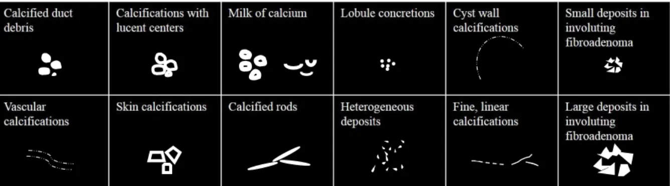
invasive ductal cancer. ... 7 Figure 1.5 Illustration of many calcification types that are observed with

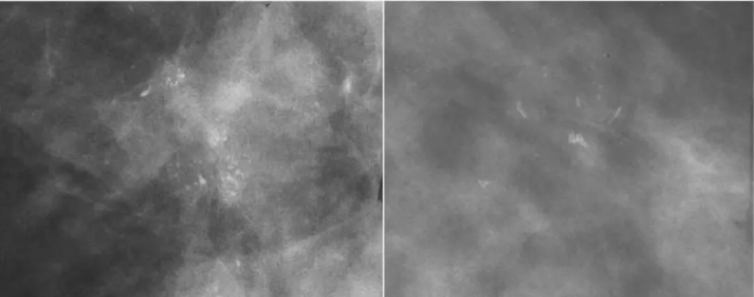
mammography. Adapted from Kopans, 2007. ... 8 Figure 1.6 X-ray examples of calcifications typical of ductal carcinoma

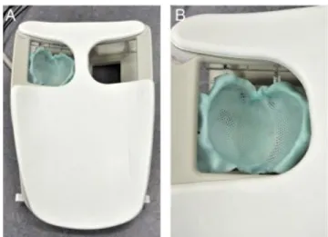
in situ. Left: Granular type. Right: Pleomorphic type. ... 9 Figure 1.7 (A) Photograph of an ultrasound unit used in a mammography

clinic. (B) Close-up of a transducer used for imaging. ... 10 Figure 1.8 Ultrasound image of a multilobulated mass that is invasive

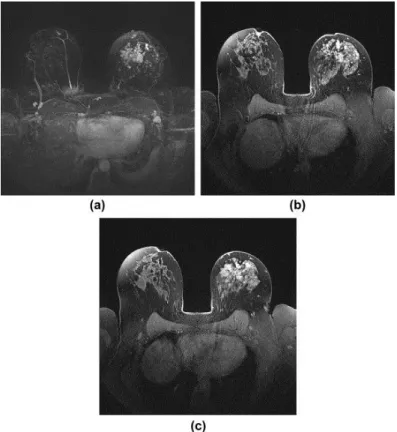
ductal cancer, but appeared round on a mammogram. ... 11 Figure 1.9 Dedicated MRI breast coil, with the coil detail shown in (B). ... 13 Figure 1.10 MRI breast image sequence of invasive lobular carcinoma

in the left breast. ... 14 Figure 1.11 Illustration of a typical Bremsstrahlung radiation spectrum

for the case of a 40 kV acceleration potential. ... 17 Figure 1.12 Illustration of a complete X-ray spectrum characteristic of a

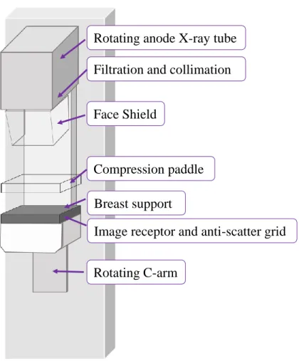
silver metal target and acceleration potential of 40 kV. ... 18 Figure 1.13 Illustration of a mammography unit with major components

labeled. Adapted from Ikeda, 2011. ... 25 Figure 1.14 Photograph of a mammography unit built by GE. ... 26 Figure 1.15 Cross-section of a mammography unit showing the details of

the X-ray tube and collimation, as well as the breast support area and

(22)

Figure 1.16 Direction lines for the CC and MLO views used in breast

imaging. ... 31 Figure 1.17 A CC-view set of X-rays placed back-to-back. The images for

each breast are placed back to back. Attribution: © Nevit Dilmen ... 32 Figure 1.18 Right and left MLO X-rays back-to-back. Attribution:

with fatty breasts. The left image (C) is an SFM image, and the right

image (A) is a DM image. ... 34 Figure 1.20 Illustration of a DBT system with major components labeled.

Example tube trajectory during imaging is indicated by the curved arrow. There is one tube head, black, that moves to different projection locations,

illustrated by the gray tube head images. ... 37 Figure 1.21 Illustration of the shift-and-add method for image

reconstruction whose principle is the basis for more complex

reconstruction methods used in DBT. This image shows how a plane

would be constructed so that the burst shape comes into focus. ... 38 Figure 1.22 Comparison of a 2D DM projection and a DBT slice for

DCIS. The spiculation and MCs are hidden in the DM image, but clearly

seen in the DBT image. ... 45 Figure 1.23 Photograph of a Hologic Selenia Dimensions DBT system in

a laboratory setting. ... 47 Figure 2.1 Illustration of a proposed s-DBT system with many X-ray

sources housed in one X-ray tube. The "x" markers indicate X-ray source locations within the tube, corresponding to projection locations that will

form the tomosynthesis reconstruction. ... 6 Figure 2.2 Illustration comparing the difference between a stationary

focal spot (s-DBT), and a blurred focal spot (DBT). The DBT focal spot gets stretched in the direction of tube travel. This illustration assumes a tube travel of 1.65 mm during an exposure in which the whole acquisition

would total 100 mAs. ... 8 Figure 2.3 Potential energy diagram at the surface of a metal under the

influence of an external electric field. ... 9 Figure 2.4 Simple schematic of a thermionic X-ray tube. Adapted from

(23)

Figure 2.6 Illustration of a Spindt field emitter array. The left image is a cross-section view, and the right image is a top view, showing the circular

gate openings. Adapted from Zhu, 2001. ... 14 Figure 3.1 The left photograph in this figure shows three CNT cathodes

of the type placed in the s-DBT system. On the right, in the red box, is a

TEM image of the type of FWNTs deposited on the cathodes. ... 37 Figure 3.2 On the left is a magnified photograph of a gate mesh

immediately after fabrication. The right photograph shows an example of a gate frame with gate mesh welded over the individual openings. This

gate frame was not for the s-DBT tube, but the gate mesh are very similar. ... 38 Figure 3.3 Optical microscope images of a tungsten gate mesh. The bar

thickness and spacing size are labeled. Also, the curved bar edges can be

seen. ... 39 Figure 3.4 Illustration of the complete electron configuration in the s-DBT

tube including simulated electron trajectories in the left-hand image. The two views are different cross-sections of the structure. Adapted with

permission from Sultana, 2010. ... 40 Figure 3.5 Complete electrode structure from the SolidWorks drawing of

the s-DBT tube. ... 41 Figure 3.6 Photographs of an s-DBT X-ray tube with key features labeled.

The orientation used in breast imaging is shown in the right photograph,

with the X-ray window facing downward toward the detector. ... 42 Figure 3.7 Schematic illustrating the difference in the real, or actual, focal

spot size and the effective focal spot size. ... 44 Figure 3.8 Schematic of the geometric configuration determining effective

anode angle with tube tilt and positioning on the gantry incorporated. ... 45 Figure 3.9 Dose rate measurements comparing the Hologic Selenia

Dimensions system to the s-DBT system. Data taken by Dr. Andrew

Tucker. ... 47 Figure 3.10 (A) Hologic Selenia Dimensions system, with a red arrow

indicating the tube motion path. (B) The s-DBT tube integrated with the Hologic gantry. Reprinted from Gidcumb et al 2014 Nanotechnology

25 245704... 48 Figure 3.11 Photograph of the completely integrated s-DBT system

including the Hologic and s-DBT controls. ... 49 Figure 3.12 Simplified electronic communication flow diagram of the

(24)

Figure 4.1 Illustration of woven and linear tungsten-wire gate mesh.

Adapted with permission from Sultana, 2010. ... 61 Figure 4.2 Optical microscope images. Left: Woven tungsten mesh.

Middle: Molybdenum with a grid of circular openings. Right: Etched, linear tungsten mesh. Images reused with permission of Xiomara

Calderòn-Colòn. ... 61 Figure 4.3 Pictures of various gate materials investigated for s-DBT. The

silicon and tungsten (straight bars) images were used with permission from Xiomara Calderon-Colon. Stainless steel and molybdenum images

are from XinRay Systems. ... 63 Figure 4.4 Illustration of the Bosch process. Adapted from Fransilla, 2010. ... 65 Figure 4.5 Photograph of the corner paste configuration that allowed for

successful mesh etching. ... 74 Figure 4.6 Photographs comparing the appearances between a failed

sample, due to photoresist damage, to a successful one. There was some photoresist damage even on the successful sample, but it did not reach the critical area containing the tungsten bars. The top of the left-most mesh

in the successful etch example was not fully etched, but the other two were. ... 74 Figure 4.7 10x magnification optical microscope images of tungsten gate

mesh corresponding to the MRT sample data presented in Table 4.4. ... 76 Figure 4.8 Optical microscope images comparing the surface roughness of

DRIE mesh and wet-etched mesh. Images taken by Derrek Spronk. ... 79 Figure 5.1 Temperature simulation results at the center of the s-DBT

tungsten anode during one X-ray pulse. The settings are for various anode currents and pulse widths, all at 38 kV anode voltage. The insert is an image of the simulated anode showing the temperature distribution at the end of a pulse with settings of: 250 ms, 28 mA anode current, and 38 kV anode voltage. Reprinted with permission from Qian et al., Med. Phys., 39, 2094, (2012). Copyright 2012, American Association of Physicists

in Medicine. ... 83 Figure 5.2 Accelerated lifetime test data using a testing module,

simulating the electrode configuration of the s-DBT X-ray tube. (A) 27 mA anode current, 250 ms pulse width, 5 % duty cycle. Inset: Shows an example cathode current pulse. (B) 38 mA anode current, 183 ms pulse width, 0.6 % duty cycle. Reprinted with permission from Qian et al., Med. Phys., 39, 2095, (2012). Copyright 2012, American

(25)

Figure 5.3 Cathode-gate voltages required to produce an average of 42.6 ± 0.4 mA for the 31 CNT cathodes in the s-DBT X-ray tube. Reprinted with permission from Qian et al., Med. Phys., 39, 2096,

Association of Physicists in Medicine. ... 87 Figure 5.5 (A) The projection MTFs of the stationary and rotating gantry

DBT systems along the scanning direction. (B) The system MTFs

Association of Physicists in Medicine. ... 88 Figure 5.6 (A) Photograph of the CIRS breast biopsy phantom. (B) - (D)

Reconstructed slices of the CIRS phantom from the s-DBT system. The depths of the slices are (B) 1 cm, (C) 2.5 cm, and (D) 4 cm from the phantom's surface. Reprinted with permission from Qian et al., Med. Phys., 39, 2097, (2012). Copyright 2012, American Association of

Physicists in Medicine. ... 90 Figure 5.7 (A) Photograph of the ACR phantom. (B) Illustration of the

objects imbedded within the ACR phantom. The yellow box indicates 0.54 mm specs, the green box indicates 0.4 mm specs, and the blue box indicates 0.32 mm specs. (C) - (E) s-DBT system reconstruction slices at (C) 0.7 cm, (D) 1.4 cm, and (E) 2 cm from the top of the phantom.

(F) – (H) s-DBT reconstruction slices at 1.4 cm for the three MC spec sizes indicated by the colored boxes. (I) – (K) The same images as (F) – (H) for the Hologic system. Reprinted with permission from Qian et al., Med. Phys., 39, 2097-98, (2012). Copyright 2012, American Association of

Physicists in Medicine. ... 91 Figure 5.8 Plots of cathode current and electric field data during field

emission testing with 0.1 Hz frequency. Cathode current settings were (A) 27 mA, (B) 41 mA, (C) 60 mA, (D) 80 mA, and (E) 78 mA. The experimental data for (A) through (D) was gathered sequentially on a single cathode using 250 ms pulse widths. The data in (E) was performed with a second cathode, and 125 ms pulse widths. Reprinted from Emily

Gidcumb et al. 2014 Nanotechnology 25 245704. ... 94 Figure 6.1 (A) SEM image of a CNT cathode. (B) Raman spectroscopy

data of a CNT sample representative of those deposited on the FWNT cathodes tested throughout this study. Data provided by Dr. Bo Gao.

(26)

Figure 6.2 (A) High-magnification TEM images of (A) CVD-grown CNTs and (B) arc-discharge CNTs. Scale bar represents 5 nm. Reprinted with permission from Koh et al., ACS Nano, 7, 2567, (2013). Copyright 2013

American Chemical Society. ... 103 Figure 6.3 Illustration of the experimental setup, not drawn to scale. The

tube housing contained three cathode-anode pairs, an example of only one is shown here. Reprinted from Gidcumb et al. 2014 Nanotechnology

25 245704... 105 Figure 6.4 I-V curves for both the MWNT and FWNT cathode. Both

current and current density are shown plotted versus electric field. FWNT

data reprinted from Gidcumb et al. 2014 Nanotechnology 25 245704. ... 109 Figure 6.5 FWNT field emission results for the 4 s pulse width testing, for

both 50 mAs and 75 mAs targets. (A) and (B) plot different quantities for the same pulses; same for (C) and (D). (A) Raw cathode current and voltage data for the 50 mAs target. Inset: One, 4 s pulse of cathode current averaging 27.6 mA, producing 61 mAs. (B) Calculated anode exposure and electric field data for the 50 mAs testing. The green lines demarcate the region considered the target exposure region. The vertical dotted lines in (A) and (B) indicate when anode voltage changed during the experiments. (C) Cathode current and voltage data for the 75 mAs testing. Inset: One, 4 s pulse of 33.5 mA cathode current, equaling 74 mAs. (D) Calculated anode exposure and electric field data for the 75 mAs testing, also with green dotted lines indicating the target region. All data in (C) and (D) was taken at 35 kV. Cathode current and applied electric field data, as well as the inset in (A) are reprinted from

Gidcumb et al. 2014 Nanotechnology 25 245704. ... 111 Figure 6.6 Field emission data for the FWNT cathode producing 3 s

pulse widths with a target of 50 mAs. (A) Plots of measured cathode current and cathode voltage. (B) Plots of calculated anode exposure and applied electric field, with the target exposure region outlined with green

dotted lines. ... 114 Figure 6.7 Field emission results for 2 s pulses. All data was taken at 35

kV. (A) and (B) show the results for cathode 1 (FW 1); (C) and (D) show the results for cathode 2 (FW 2). An example 2 s pulse is shown in the inset of (C). The pulse had an average current of 44.5 mA, equaling an exposure of 49 mAs. It can be seen that the anode exposure in (B) never

reached the target region, outlined by the green dotted lines. ... 116 Figure 6.8 Field emission data for 4 s pulses produced from the MWNT

(27)

anode current measurements. (B) Anode exposure and applied electric field calculations, with the target exposure region outlined with green horizontal lines. The inset in (B) shows an anode current pulse 4 s long,

averaging 13.7 mA, totaling 50 mAs. ... 118 Figure 6.9 Field emission results for the 3 s experiments done with the

MWNT cathode. (A) Cathode and anode current data, as well as cathode voltage data. (B) Calculated anode exposure and applied electric field data. Inset: A 3 s anode-current pulse averaging 18.3 mA, equaling 50

mAs. ... 119 Figure 6.10 Field emission results for the 2 s, 50 mAs testing done with

a MWNT cathode. (A) Measured cathode current, anode current, and cathode voltage data for each pulse. (B) Calculated anode exposure and applied electric field for each pulse. Inset: An example 2 s pulse with an

average anode current of 24.2 mA, totaling an exposure of 49 mAs. ... 120 Figure 6.11 SEM images of cathode FW 1 after use in field emission

experiments. (A) and (B) are profile images, where the SEM sample was tilted approximately 90°. (C) and (D) are top-view images, looking

straight on the cathode surface. ... 122 Figure 6.12 SEM images of cathode FW 2 after being removed from the

testing chamber, where it underwent conditioning and 2 s pulse testing.

(A) and (B) are profile views, and (C) and (D) are top views. ... 123 Figure 6.13 SEM images of the third FWNT cathode in the testing

chamber that only underwent conditioning. (A) and (B) are side-view images. (C) and (D) are top-view images. (D) is a low magnification

image showing unusual pock marks or melting. ... 124 Figure 6.14 (A) SEM image of surface damage of the third FWNT

cathode. Pink outline indicates where the EDS spectrum was taken. The scale bar represents 80 µm. (B) EDS spectrum from the area in (A), taken

at 20 kV and 12 mm working distance. ... 125 Figure 6.15 SEM images of the MWNT cathode before it was used for

field emission measurements. (A) and (B) are profile views. (C) and (D)

are top views. The scale bar in (D) is 3 µm. ... 126 Figure 6.16 SEM images of the MWNT cathode after it was used for

field emission measurements. (A) and (B) are profile views. (C) and (D)

are top views. ... 127 Figure 6.17 Optical microscope images of the gate mesh above cathode

(28)

Figure 6.18 Optical microscope images of the gate mesh above cathode

FW 2... 129 Figure 6.19 Optical microscope images of the gate mesh above the third

FWNT cathode in the testing chamber, only used during conditioning. ... 130 Figure 6.20 Optical microscope images of the gate mesh above the MWNT

cathode used in field emission experiments. ... 131 Figure 7.1 Plot of the ASF of a 14° angular span (red) and of a 28°

angular span (blue). Number of projection images and total entrance dose were held constant. Reprinted with permission from Tucker et al., Med. Phys., 40, 031917-8, (2013). Copyright 2013, American Association

of Physicists in Medicine. ... 137 Figure 7.2 FWHM of ASF data at various angular spans. Reprinted with

permission from Tucker et al., Med. Phys., 40, 031917-8, (2013).

in Medicine. ... 139 Figure 7.4 Cathode voltages required to produce approximately 39 mA

cathode current, for each of the 31 s-DBT system cathodes, at two different points measured in Dec. 2010 and Nov. 2012. This data demonstrates that all 31 cathodes in a working s-DBT tube can reliably operate for several years. Dec. 2010 data provided by Derrek Spronk.

Reprinted from Gidcumb et al. 2014 Nanotechnology 25 245704. ... 141 Figure 7.5 Plot of the transmission rate, in fraction form, for each cathode

in the s-DBT prototype X-ray tube at various dates. The legend entry contains the date the data was taken in month and year, followed by the cathode current. Sept. 2011 data provided by Andrew Tucker. Reprinted

from Gidcumb et al. 2014 Nanotechnology 25 245704. ... 143 Figure 7.6 (A) Reconstructed slice from the s-DBT system of a breast

specimen with a suspicious mass. (B) 2D magnification image of the same breast specimen. Reprinted with permission from SPIE. Tucker et al., Comparison of the diagnostic accuracy of stationary digital breast tomosynthesis to digital mammography with respect to lesion

characterization in breast tissue biopsy specimens: a preliminary study,

Proc. of SPIE, Vol. 8668, 2013. ... 146 Figure 7.7 (A) Reconstruction slice of a specimen with a large cluster of

(29)

DBT system. (C) Zoomed-in area of the MC cluster as indicated by the blue box in (A). (D) Zoomed-in area of the same MC cluster imaged with the CTM DBT system. Reprinted with permission from SPIE. Tucker et al., Increased microcalcification visibility in lumpectomy specimens using a stationary digital breast tomosynthesis system, Proc. of SPIE,

2014... 148 Figure 7.8 Regions of interests around the first 6 chosen MCs. The s-DBT

images are in the top row, and the CTM DBT images are in the bottom row. Reprinted with permission from SPIE. Tucker et al., Increased microcalcification visibility in lumpectomy specimens using a stationary

digital breast tomosynthesis system, Proc. of SPIE, 2014. ... 149 Figure 7.9 Reconstructed CC image slices of Patient 1 at heights of (A)

13.5 mm and (B) 26.5 mm. The red and yellow boxes illustrate different objects coming into focus at different heights. The red box shows a mass marked by a metal biopsy clip, and the yellow box shows a

microcalcification cluster. Total exposure was 91 mAs over 15

projections, with a peak voltage of 34 kVp. ... 151 Figure 7.10 A reconstructed MLO slice from Patient 1, at 16.5 mm, with

the same areas highlighted in yellow and red as in Figure 7.9. Total

exposure was 97 mAs over 15 projections, with a peak voltage of 38 kVp. ... 152 Figure 8.1 Representative beam profile exhibiting shift in focal plane

along the axial direction with change in Focus 2 aperture. Figure reprinted

with permission from S. Sultana, PhD thesis, 20101_{. ... 155}

Figure 8.2 Illustration showing directional naming conventions. The short and long side of the cathode gave rise to the terms short and long side of the focal spot size. The short side corresponds to the scanning direction, and the long side corresponds to the non-scanning direction. The right

side of the picture is a top-view of the detector plane. ... 157 Figure 8.3 Photos of the experimental setup. (A) Top-view of the MTF

cross-wire phantom attached to the breast compression paddle. A line pair phantom is also present. (B) Side-view of the setup showing the display on the gantry, used for relocating the paddle after each image. (C) Front-view showing the phantom suspended below the compression paddle. (D) ACR phantom, after the top and wax insert were removed, was used to level the compression paddle so that it was parallel to the

detector surface. ... 161 Figure 8.4 Example image taken during the experiments, with each item

(30)

The orange box shows the region of wire used to measure MTF in the

x-direction, and the blue box is that for MTF in the y-direction. ... 162 Figure 8.5 Example data analysis of the image shown in Figure 8.3 from

beam P11 for MTF in the x-direction. (A) The resultant oversampled LSF produced from many LSFs along the wire ROI and adjusted for wire angle. (B) MTF resulting from the FT of the oversampled LSF in (A), with

a 10 % value of 7.6 cycles/mm. ... 164 Figure 8.6 Plot of all applied focusing settings tested using beam P11 to

narrow down an area to test the 15-beam set. The point outlined in orange is the grounded setting. The purple-outlined points were selected

for testing all 15 beams. ... 167 Figure 8.7 MTF product results for all settings from P11 images. MTF

product is in (cycles/mm)2 and plotted versus VAppl on F2. (A) Results

for the most negative VAppl settings on F1. (B) Results for more positive

settings on F1. Results were separated for better data visualization... 169 Figure 8.8 Color figures giving 2D distribution of MTF magnitudes over

applied focusing voltages. (A) MTF product results. (B) X-direction only.

(C) Y-direction only. Color bars to the right provide scaling information. ... 170 Figure 8.9 Transmission rate results for beam P11 at all tested focusing

voltages. (A) and (B) separate the results according to more negative and positive VAppl settings on F1, respectively. (C) 2D color distribution of

TR results, with the magnitude scale bar to the right. ... 171 Figure 8.10 MTF product results. Results for each cathode/projection are

given for each setting. Coloring from green to red indicates the settings

with the highest to the lowest all-beam average MTF product. ... 176 Figure 8.11 Simulation results showing FSS area to be weakly dependent

on F1 voltage. Anode voltage was 30 kV, gate voltage was 1250 V

producing 20 mA. Data reprinted with permission from Shabana Sultana1. ... 178 Figure 8.12 Simulation of projection MTF curves based on focal spot size.

The blue curve results from a focal spot of 0.985 mm, and the purple curve corresponds to a focal spot size of 0.6 mm. All other settings are the same, and are the parameters used in these experiments. The 10 %

(31)

LIST OF ABBREVIATIONS AND SYMBOLS

2D Two-dimensional

3D Three-dimensional

Å angstrom

a-Se Amorphous selenium

𝑎 Constant in the Fowler-Nordheim equation

A ampere

AC Alternating current

AEC Automatic exposure control

Ag silver

Al aluminum

Ar argon

ART Algebraic reconstruction technique ASF Artifact spread function

𝑏 Constant in the Fowler-Nordheim equation

B boron

Be beryllium

BI-RADS Breast Imaging-Reporting and Data System

Br bromine

c Speed of light

C Coulomb or carbon

CC craniocaudal

(32)

CHANL Chapel Hill Analytical and Nanofabrication Laboratory

Cl chlorine

cm centimeter

CNT Carbon nanotube

Co cobalt

cp Temperature-dependent heat capacity

CR Computed radiography

CsI Cesium iodide

CT Computed tomography

CTM Continuous tube motion

Cu copper

CVD Chemical vapor deposition

d Distance from cathode to gate

D dose

Dair Dose in air

DBT Digital breast tomosynthesis

DC Direct current

DM Digital mammography

DMIST Digital Mammography Imaging Screening Trial DQE Detective quantum efficiency

DRIE Deep reactive ion etching

DRR Dynamic Reconstruction and Rendering

(33)

E energy or effective focal spot length Eeff Effective field at CNT tip

Emacro Macroscopic electric field

ECM Electro-chemical machining

EDS Energy-dispersive X-ray spectroscopy EPD Electrophoretic deposition

ESF Edge spread function

ETEM Environmental transmission electron microscope

𝑓 Spatial frequency

F Applied electric field or fluorine

F1 Focusing 1

F2 Focusing 2

FBP Filtered backprojection

FDA Food and Drug Administration

Fe iron

FFDM Full field digital mammography

FT Fourier transform

FWHM Full width at half maximum

FWNT Few-wall nanotube

g gram

Gy gray

H hydrogen

(34)

hr hour

HV High voltage

Hz Hertz

I Intensity of monoenergetic X-rays exiting a material or emission current

I0 Initial monoenergetic intensity

ITO Indium tin oxide

J Joule or current density

𝑘 Boltzmann constant or emitter shank variable

K Kelvin

keV kiloelectronvolt

kg kilogram

kVp Kilovolt peak

lb pound

Li lithium

LSF Line spread function

lp Line pairs

m meter

mA milliampere

mAs Unit current in mA times unit time in seconds

MC microcalcification

MeV megaelectronvolt

mg milligram

(35)

mGy milligray

min minute

MITS Matrix inversion tomosynthesis

mL milliliter

MLEM Maximum likelihood expectation maximization method MLO Mediolateral oblique

mm millimeter

Mo molybdenum

MQSA Mammography Quality Standards Act

mR milliRoentgen

MRI Magnetic resonance imaging MRT Microbeam radiation therapy MTF Modulation transfer function MTFX MTF in the x-direction

MTFY MTF in the y-direction

MWNT Multi-wall nanotube

n Number of photons removed

N Number of incident photons or number of transmitted photons or nitrogen

N0 Number of incident photons

nA nanoampere

Ni nickel

nm nanometer

(36)

NMR Nuclear magnetic resonance

O oxygen

ODD Object-to-detector distance

Pin Input power

Prad Output power from blackbody radiation

PCM Photochemical machining

PET Positron emission tomography

pm picometer

PSF Point spread function

r emitter radius

R Roentgen or emitter-gate distance or real focal spot length

rad Radiation absorbed dose

RF Radio frequency

Rh rhodium

RIE Reactive ion etching ROI Region of interest rpm Revolutions per minute

RTT Real Time Tomography

s second

S sulfur

S0 Initial polyenergetic spectrum

(37)

SART Simultaneous algebraic reconstruction technique SDNR Signal difference-to-noise ratio

SFM Screen film mammography

SI International System of Units

Si silicon

SID Source-to-image receptor distance

SIRT Simultaneous iterative reconstruction technique SNR Signal-to-noise ratio

SOD Source-to-object distance SSM Step-and-shoot motion

SWNT Single-wall nanotube

t time

T temperature

Tm Melting temperature

TEM Transmission electron microscopy

Ti titanium

TR Transmission rate

U.S. United States

US ultrasound

UNC University of North Carolina at Chapel Hill

UV ultraviolet

V Applied voltage or Volt

(38)

VCath Cathode voltage

VRel Relative focusing voltage

W tungsten or Watt

x thickness or distance

X exposure

z Focal plane location

Z Atomic number

Zn zinc

 Wavelength of electromagnetic radiation  Frequency of electromagnetic radiation

ℎ Planck’s constant

 Linear attenuation coefficient or Fermi level Δx Small, discrete unit of length or thickness

 density

 Energy fluence

𝜇𝑒𝑛

𝜌0 Mass energy absorption coefficient

 fluence

ϕ Work function

β Field enhancement factor

µm micrometer

µA microampere

θ Anode angle

(39)

∇ gradient

Ω Ohm

𝜇_𝑏𝑘𝑔 Average value of background pixels

𝑥̅ Average value of parameter x

δx Error of parameter x

(40)

CHAPTER 1: INTRODUCTION

1.1 Importance of breast imaging

The lifetime risk for a woman in the United States of being diagnosed with breast cancer is one in eight1. In 2013, in the United States, invasive female breast cancer accounted for 29 % of all new cancer cases and 14 % of all cancer related deaths2_{. In addition to the}

estimated 232,340 new invasive breast cancer cases, 64,640 in situ diagnosed cancer cases were estimated in 2013. In situ cancers only have cells at the initial cancer site, whereas invasive cancerous cells have moved beyond the initial tissue layer2. It is hoped that, through screening efforts, cancers can be detected while in situ, before the cancer begins spreading1.

Breast cancer screening, comprised of a clinical breast exam and mammography for women aged 40 and over, helps save lives by catching cancers as early as possible2. There is a positive correlation between cancer stage at the time of diagnosis and the 5-year relative survival rate of cancer patients to people without cancer1_{. If the cancer is localized at the time}

of diagnosis, the survival rate is 99 %. But, if the cancer is distant from the original site, the 5-year relative survival rate lowers to 24 %. From the 1980’s to the 1990’s breast cancer screening caused the breast cancer incidence rate to increase, but have since then stabilized. Over the 20 years from 1990 to 2010, mortality decreased by 34 % due to a combination of early detection and improved treatments1_{. Breast cancer screening does save lives, but cancer}

(41)

In addition to screening, diagnostic imaging is a very important part of breast imaging. Effective patient care must include both the accurate detection and diagnosis of cancer. The main purpose of screening is to detect the presence of disease, but diagnosis is needed to determine whether the disease is malignant or benign3. Typically, if cancer is detected through mammography, biopsies are done in order to properly diagnose the cancer. The role of breast imaging is to clearly confirm the presence of a suspicious lesion, but it can only aid in diagnosis if the lesion presents with visual indications of being benign or malignant. For example, certain calcification arrangements can be such an indicator. Breast imaging plays an important role in both effectively detecting cancer and helping to rule out malignancy, in order to reduce the number of breast biopsies returning negative results3.

1.2 Motivation for improving breast imaging

Although mammography is a powerful tool in saving lives, there are notable

drawbacks. Today, mammography is primarily dominated by X-ray imaging. Unfortunately, it is not 100 % accurate, and accuracy is worse for women with dense breasts2. Women who may never get cancer in their lifetime are subject to regular screenings, and many will go through false alarms1. Studies find varying rates, of up to 30 %, of the over diagnosis of cancers that would not have progressed and report the rate of biopsies corresponding to false positives at 19 %1. In Europe, about 200 out of 1,000 patients receive false positives4

(42)

In addition to X-ray mammography, magnetic resonance imaging (MRI) and

ultrasound (US) are used to supplement the screening and diagnosis of breast cancer for some patients. Both of these modalities have their own advantages and drawbacks. A study of 617 patients in the Czech Republic showed that results from preoperative workups, including all three modalities plus core needle biopsy, were significantly different than postoperative histology findings for tumor size, multifocality, and suspicious lymph node status6. Current mammographic techniques and procedures have greatly increased breast cancer survival rates, but there are many drawbacks that make further improvements necessary.

Among the three imaging modalities of X-ray, MRI, and US, X-ray imaging remains the most heavily used method for evaluating breast cancer and is the application that is the focus of this work. The motivation for improving X-ray mammography lies in helping to increase accuracy, resulting in lowering treatment costs and improving the patient’s quality of life.

1.3 Mammography

1.3.1 Mammographic features

Mammographic features of interest for determining the presence of breast cancer include masses, calcifications, architectural distortions, asymmetries, and any changes in those since previous images were taken3.

1.3.1.1 Masses

(43)

they affect surrounding tissues3. Figure 1.1 gives an illustration of the various types of mass shapes as well as various types of margins masses can have.

Round, oval, and lobulated masses tend to have circumscribed margins that are sharp and clear3. Benign lesions tend to be round and circumscribed. Less than 10 % of breast cancers have smooth shapes and margins. An example of a cancerous, round mass can be seen in Figure 1.2 17_{. The mass required US for diagnosis, highlighting the diagnostic}

limitations of 2D X-ray mammography. Benign lesions tend to be fibroadenoma, cyst, abscesses from infection, Phyllodes Tumors, papilloma, or fat-containing masses, and are very rarely cancers including metastasis from another cancer elsewhere in the body3,7.

The appearance of normal lymph nodes on a mammogram are usually oval and fatty, but an abnormal lymph node that would indicate cancer spreading would be larger, rounder, and non-fatty7. Typically, benign lymph nodes, cysts, and scars are left un-biopsied if

1_{This image was published in Breast Imaging: The Requisites, 2}nd_{Edition, Debra M. Ikeda, Chapter 4, Page}

115, Copyright Elsevier (2011).

(44)

margins can be clearly identified as regular shaped, and well circumscribed7. Therefore, having good spatial resolution in imaging is important to clearly define the edges of structures, such as masses and lymph nodes.

Malignant lesions are defined as those that invade the surrounding tissue, and

therefore tend to have irregular shapes and margins7_{. Obscured margins usually end up being}

biopsied because, due to overlapping tissue, it is unclear whether the mass shape is regular or irregular3,7. Lobulated masses have a high probability of being benign, but a micro-lobulated margin, where the shape irregularities are on the order of millimeters, could be the result of a growing cancer, as shown in Figure 1.3 23_{. Ill-defined or indistinct margins suggest that a}

malignancy is spreading to surrounding tissue, and requires biopsy3,7_{. Finally, spiculated}

margins indicate the growth of cancer cells into the surrounding tissues, and is a key

(45)

indicator for malignancy7. Types of cancers that present with spiculated margins include invasive ductal cancer, invasive lobular carcinoma, and tubular cancer. Other lesions can appear with spiculations, but may not be cancer, such as scars and fat necrosis7.

Being able to clearly see the outline of a mass is a very important part of breast cancer screening and may require additional views, as shown in Figure 1.4 3_{. Overlapping}

tissue can blur lesion margins, and spiculated or irregularly shaped masses could have fine details that need to be differentiated in an image. Therefore, mammographic image quality and the ability to remove surrounding tissue overlap is very important for determining the presence of cancer.

(46)

1.3.1.2 Calcifications

Another key feature that radiologists look for in a mammogram is calcifications, examples are illustrated in Figure 1.5. Most calcifications that form in the breast are benign, but 50 % – 80 % of all cancers are associated with calcifications and are sometimes the only visible sign of cancer on the mammogram7. Cancerous calcifications develop from tumor center necrosis or secretions from malignant cells. Important factors to look for are the individual shape of a calcification, and the shape and location of the calcification cluster. In general, calcifications that are located in the breast ducts, lobules, and inside tumors are malignancy indicators7. A mass that has other malignant indicators has an increased chance of being cancerous if calcifications are also present3. If the calcifications are located within interlobular stroma, outside of ducts, or in the blood vessels, fat, muscle, nipple, or skin, they are typically benign7.

(47)

Calcifications that are easily labeled as benign are any with lucent centers, that are less X-ray absorbent, and include those found in fat necrosis or in the skin3. Other benign calcifications are those found in cysts, either egg-shell type on a cyst wall or those referred to as milk of calcium. Any calcifications formed into rods due to secretory disease or present in involuting fibroadenoma are benign. Typically, benign calcifications are calcified debris in ducts, concretions in dilated lobules, and vascular calcifications. If duct debris begins to form a spherical cluster over time, they could be a cause for concern3_.

Cancerous calcifications are typically less than or equal to 0.5 mm in size, irregularly shaped, and vary in shape and size within a cluster3. Heterogeneous deposits, also known as pleomorphic or granular deposits, are not typical of anything but are suspicious if they meet the qualifications for cancerous calcifications. An example of these calcifications is shown in Figure 1.64_{, where they were indicative of ductal carcinoma in situ. Fine, linear}

calcifications, less than 1 mm in size, are usually present in necrotic tumors. They are thin, irregularly shaped, and made up of discrete, discontinuous calcifications3. Therefore, spatial

4_{This image was published in Breast Imaging: The Requisites, 2}nd_{Edition, Debra M. Ikeda, Chapter 3, Page 87,}

(48)

resolution and image quality for mammograms are very important because cancerous calcifications are generally smaller and more difficult to see.

1.3.2 Non-radiographic imaging modalities used with mammography

Although neither ultrasound nor MRI are recommended for general breast cancer screening at this time, there are many uses for both modalities to supplement current mammography practices7.

1.3.2.1 Ultrasound

Ultrasound (US) imaging combines the properties of high-frequency sound waves and the acoustic properties of the body8. A transducer is used to emit short ultrasound pulses into the tissue it is physically in contact with, as shown in Figure 1.7. The sound waves interact with the tissue which reflects an echo back to the transducer, especially at object surfaces and internal structures. The echoes are detected along linear paths over different angles in the area being imaged, known as sector scanning. The images produced are on a gray scale proportional to the echo amplitude detected, and depth of the object can be determined by the time difference between when the echo is measured and when the original pulse was

(49)

produced. Two-dimensional (2D) tomographic images, or three-dimensional (3D) images can be produced through US8_.

If a clinical breast exam or screening mammography return abnormal findings, US can be used in a follow-up exam, as in the Figure 1.8 5_{,used to follow up on the lesions}

shown in Figure 1.29_{. For example, US could be used to further evaluate calcifications found}

on a mammogram to see if there is a mass associated with the calcifications that was invisible to X-rays7. Screening is done with ultrasound for women younger than 30 if they have a palpable mass and for women of any age with dense breasts7. For women who have dense

(50)

breasts, US can be useful to remove the obstruction from overlying tissues that would be a problem in digital mammography10_{. It has been shown that using whole breast screening US}

in combination with mammography can increase the detection of cancers in women with dense breasts by 55 %9. One major use for US is in differentiating solid masses from cysts7,11. Cysts make up about 25 % of all detected breast lesions11, but are benign7. However, a solid mass could be either benign or malignant7. To evaluate the presence of cancer in a solid mass, US is used to determine the mass shape, margins, thickness of the echogenic rim, duct extension, how the mass affects surrounding tissue, if it is taller than wide, and its acoustic properties. If a mass is taller than it is wide, that indicates the mass is growing outside of its initial tissue plane, and is a sign of malignancy7. Other main uses of US include image guidance for percutaneous needle biopsies7 and decision making for surgery and therapy planning10_.

Additionally, ultrasound is very useful because it is a fast and easy method that can be carried out with handheld transducer devices7. It does not involve ionizing radiation; only

(51)

employs moderate compression, if any; and is widely available7. However, there is currently not enough evidence to prove that US alone is adequate for general breast cancer screening9_.

Although some lesions that are missed in mammography can be seen with US, there are lesions, both cancerous and non-cancerous, that cannot be seen with US7. Ultrasound is also limited in its effectiveness for fatty breasts and for visualizing most calcifications7.

1.3.2.2 Magnetic resonance imaging

MRI generates images by localizing nuclear magnetic resonance (NMR) signals using magnetic field gradients8. NMR signals originate from the magnetic properties inherent to the nuclei of atoms with nonzero nuclear magnetic moments. When the nuclei are placed in a strong, external magnetic field and exposed to radiofrequency (RF) pulse sequences, they absorb and emit a characteristic energy that is used to identify the location and quantity of the particular nuclei of interest. An example of a dedicated MRI coil for the breast can be seen in Figure 1.96_{. The characteristic energy signals are then reconstructed into MR images with}

high levels of soft tissue contrast, adjustment made possible through the development of increasingly complex pulse sequences. The images are 3D and viewed as sets of tomographic slices through the imaged portion of the body. Due to their different local magnetic

properties, MRI can differentiate materials such as fat, brain matter, fluids, and cancer8_.

(52)

MRI is primarily used in breast cancer screening for women who are at a higher risk of breast cancer for reasons such as having a family history of breast cancer9, testing positive for the BRCA1 and BRCA2 genetic mutations9, women with a history of Hodgkin disease7, and women with a greater than 20 % lifetime risk of developing cancer7_{. Women with silicon}

breast augmentation are also screened with MRI7, because the silicon does not cause

extensive artifacts in MRI nor prohibit imaging the surrounding breast tissue as it does with mammography.

Certain lesions are only visible on MRI7, such as some cases of ductal carcinoma in situ and some cases of multifocal disease10_{; and it is the most accurate and sensitive for}

evaluating tumor extent10. With a 93 % sensitivity rate, it is also the most sensitive modality for the preoperative staging of invasive lobular carcinoma10. Invasive lobular carcinomas that cannot be seen with mammography can generate a high signal intensity in MRI when using contrast agents7, giving information on the lesion’s vascularization10. An example of an MRI

(53)

image showing invasive lobular carcinoma can be seen in Figure 1.107_{. Other main uses of}

MRI for the breast include image-guided core biopsies and needle localization for surgery. It is also used to evaluate patients’ response to chemotherapy and to evaluate the recurrence of cancers7.

One of the main drawbacks of MRI is its cost, playing a large part in its infrequent use in breast screening in general7. Another issue is the tendency of MRI to overestimate a lesions’ malignancy, giving it a large specificity range of 39 % to 95 %. These false positives

7_{Reprinted from Clinical Radiology, 69, M. Muttalib, R. Ibrahem, A.S. Khashan, M. Hajaj,} Prospective MRI assessment for invasive lobular breast cancer. Correlation with tumour size at histopathology and influence on surgical management, Page 27, Copyright (2014), with permission from Elsevier.

(54)

can be due to lesions that, in MRI, mimic ductal carcinoma in situ or invasive carcinoma. Some of the types of lesions that cause issues are fibroadenoma and papilloma. MRI is also subject to many types of artifacts, including motion of the patient and motion from cardiac and respiratory processes7. In addition to the imaging shortcomings due to the modality itself, and even with its high sensitivity, MRI would not be used for general population screening because of the expense and limited access relative to X-ray imaging9.

1.3.3 Current state of X-ray mammography

Before going into the details of X-ray mammography, a summary of the physical principles of X-rays will be given.

1.3.3.1 The physics of X-ray imaging 1.3.3.1.1 Electromagnetic radiation

X-rays are a type of electromagnetic radiation that originate outside an atom’s nucleus and are known as ionizing radiation8. Ionizing radiation has enough energy in each photon to be able to remove electrons from their atomic orbits. All types of electromagnetic radiation can behave either as waves having a wavelength, frequency, and amplitude, or as particles of a specific energy, known as photons. The wavelength of an X-ray is determined by its speed and frequency according to the equation:

𝜆 = 𝑐 𝜈

where  is the wavelength in meters (m), 𝑐 is the speed of light defined as 3.0 × 108_{m/s, and}

 is frequency in hertz (Hz)8_{. The energy of a photon is defined as:}

𝐸 = ℎ𝜈

where E is the photon energy in Joules (J), and ℎ is Planck’s constant equal to 6.626 × 10-34

(55)

X-rays have high frequencies, short wavelengths, and range in energy from the keV to the MeV range12_{. For imaging, wavelengths range from 10 pm – 100 pm and energies}

range from 12.4 keV – 124 keV13. 1.3.3.1.2 Production of X-rays

X-rays are produced when electrons interact with matter so that some of the kinetic energy of the electron is lost8. The lost kinetic energy is converted to electromagnetic radiation in the form of X-rays. For this process to occur there must be an electron source, a vacuum environment, a target material, and an energy source to accelerate the electrons toward the target material8.

Bremsstrahlung

Bremsstrahlung means “breaking radiation”8_{. This type of X-ray can have any energy}

(56)

Characteristic radiation

Electrons surrounding atomic nuclei are ordered according to binding energies and are labeled according to different energy shells8. Going from highest binding energy and closest to the nucleus, to lower binding energy farther away, the shells are labeled K, L, M, and N. Each element has characteristic energy levels for each of their electron shells,

revealing the source of the name characteristic radiation. If an electron or Bremsstrahlung X-ray has an energy higher than the binding energies of the target material, there is the

opportunity for characteristic radiation to be produced by ejecting an electron from its orbit8. Upon ejection from its energy shell, an electron leaves an unstable “hole” in the electron cloud that is quickly filled by an electron from a shell of lower binding energy8. As the electron moves to a shell with higher binding energy, energy is lost by the electron via a characteristic X-ray. The energy of the X-ray is equal to the difference in the binding

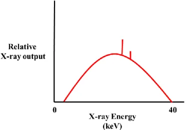
energies of the final and initial shells. These X-rays show up on the X-ray spectrum as peaks X-ray Energy

(keV) Relative

X-ray output

0 40

Figure 1.11 Illustration of a typical Bremsstrahlung radiation spectrum for the case of a 40 kV

(57)

located at the energies characteristic to the electron shell transitions. For the energy ranges relevant to imaging, the peaks seen are usually K-shell peaks8_.

Figure 1.12 shows an illustration of a spectrum from a silver target with an

accelerating potential of 40 kV. In the figure, the Bremsstrahlung radiation is filtered by the X-ray window of the tube, aluminum for example. Some energies are completely absorbed by the window, explaining why there are no X-rays at the lowest energies. Two characteristic K peaks can be seen adding on top of the Bremsstrahlung radiation. If, for example, the target material was tungsten, the K-peaks would not be visible because the binding energy of the tungsten K-shell is higher than that of a 40 kV accelerating potential. Because the

acceleration potential is 40 kV, this spectrum would be referred to as a 40 kVp spectrum. The spectrum contains a wide range of energies, but peaks at 40 kV.

(58)

1.3.3.1.3 Interaction of X-rays with matter

Once X-rays are produced in a medical imaging device, they are directed toward the patient, where the rays will interact with body tissues. There are three main ways that X-rays of energies relevant for breast imaging interact with matter: Compton scattering, Rayleigh scattering, and the photoelectric effect8,12.

Compton scattering

Compton scattering occurs when an X-ray photon interacts with an individual valence electron, ionizing the atom by knocking the electron out of its orbit8,12. The incident photon is scattered at some angle and changes direction12. The scattered photon energy is the difference between the incident photon energy and the scattered electron’s kinetic energy, and is

dependent on the photon scattering angle8,12. This type of interaction dominates the others within the diagnostic imaging range, and leads to image degradation8_{. At breast imaging}

energies, most of the energy stays with the scattered photon, reducing attenuation contrast from the primary photons. The probability of forward scattering, which impacts image quality most, is increased at higher energies8.

Rayleigh scattering

Rayleigh scattering occurs when an incident X-ray photon excites all of an atom’s electrons into a coherent oscillation that mimics the oscillation of its electric field8,13. Each of the electrons quickly emit radiation of the same wavelength as the incident X-ray. Those emitted X-rays combine into one scattered X-ray photon of the same wavelength traveling at a different angle relative to the incident photon. During this process the atom does not become ionized, and no energy is lost to kinetic energy8,13_{. The chance of this type of}