5678.pdf

(1)

VARIABLE SELECTION, SPARSE

META-ANALYSIS AND GENETIC RISK

PREDICTION FOR GENOME-WIDE

ASSOCIATION STUDIES

Qianchuan He

A dissertation submitted to the faculty of the University of North Carolina at Chapel Hill in partial fulfillment of the requirements for the degree of Doctor of Philosophy in the Department of Biostatistics.

Chapel Hill 2012

Approved by:

Dr. Danyu Lin

(2)

c 2012 Qianchuan He

(3)

Abstract

QIANCHUAN HE: Variable Selection, Sparse Meta-Analysis and Genetic Risk Prediction for Genome-Wide Association Studies

(Under the direction of Dr. Danyu Lin and Dr. Hao Helen Zhang)

Genome-wide association studies (GWAS) usually involve more than half a mil-lion single nucleotide polymorphisms (SNPs). The common practice of analyzing one SNP at a time does not fully realize the potential of GWAS to identify multiple causal variants and to predict risk of disease. Recently developed variable selection methods allow the joint analysis for GWAS data, but they tend to miss causal SNPs that are marginally uncorrelated with disease and have high false discovery rates (FDRs). Ge-netic risk prediction becomes highly challenging when the number of causal variants is large and many of the effects are weak. Existing methods mostly rely on marginal regression estimates, and their prediction power is quite limited. In meta-analysis, the involvement of multiple studies adds one more layer of complexity to variable selection. While existing variable selection methods can be potentially applied to meta-analysis, they require direct access to raw data, which are often difficult to be obtained.

(4)

Simulation studies demonstrate that the GWASelect performs well under a wide spec-trum of linkage disequilibrium patterns and can be substantially more powerful than existing methods in capturing causal variants while having a lower FDR.

In the second part, we propose a new approach, Sparse Meta-Analysis (SMA), which performs variable selection for meta-analysis based solely on summary statistics and allows the effect sizes of each covariate to vary among studies. We show that the SMA enjoys the oracle property if the estimated covariance matrix of the parameter estimators from each study is available. We also consider the situations in which the summary statistics include only the variances or no variance/covariance information at all. Simulation studies and real data analysis demonstrate that the proposed methods perform well. Since summary statistics are far more accessible than raw data, our methods have broader applications in high-dimensional meta-analysis than existing ones.

(5)

Acknowledgments

I would like to express my deepest gratitude to my advisor, Dr. Danyu Lin, for his patience, caring and guidance. To me, he has been a role model in many ways. It is truly a privilege for me to have the opportunity to work with him and to learn from him. Without him, I would never have the opportunity to conduct the research presented in this dissertation.

I am extremely grateful to my co-advisor, Hao Helen Zhang, for her great guidance and tremendous help on my research projects. I am always impressed by her scope of knowledge and creative thinking, and I thank her for allowing me to work on these highly interesting projects that she has co-developed.

I am grateful as well to my committee members, Dr. Donglin Zeng, Dr. Michael Wu and Dr. Christy L. Avery, who have helped me to significantly improve my work. I thank them for generously giving their time and expertise on my dissertation projects. I particularly thank Dr. Avery for generously sharing with me many large data sets for my research.

I thank all my friends at Chapel Hill who have helped me in the past five and half years. I cherish the friendship with them for ever.

(6)

List of Tables

2.1 True and false discoveries of variable selection methods when the model sizes are fixed at 15 (except for the ATT method) . . . 31 2.2 Prediction accuracy of variable selection methods when the model sizes

are fixed at 15 (except for the ATT method) . . . 32 2.3 True and false discovery rates when cross validation is incorporated into

variable selection (except for the ATT method) . . . 34 2.4 Prediction accuracy of variable selection methods with cross-validation

incorporated (except for the ATT method) . . . 35 2.5 List of SNPs selected by the GWASelect for the WTCCC-T2D . . . . 39 2.6 List of SNPs selected by the d-GWASelect for the WTCCC-T1D . . . . 41 2.7 Prediction errors for the WTCCC-T1D . . . 41 2.8 True and false discovery rates when the deviance is used as the evaluation

criterion for cross-validation (except for the ATT method) . . . 46 2.9 Prediction accuracy when the deviance is used as the evaluation criterion

for cross-validation (except for the ATT method) . . . 47 2.10 List of SNPs selected by different methods for Bipolar Disorder (BD) . 48 2.11 List of SNPs selected by different methods for Coronary artery disease

(CAD) . . . 49 2.12 List of SNPs selected by different methods for T1D . . . 50 2.13 List of SNPs selected by different methods for T2D . . . 51 2.14 The replication rates for different methods on the WTCCC data . . . 52 2.15 The AUC achieved by different methods for the WTCCC-T1D data on

genetic prediction (two different model sizes were evaluated for the Wu et al. model and the HLASSO model) . . . 52 3.1 Comparison of the SMA and other methods under the heterogeneous

(11)

3.2 Comparison of the SMA and other methods under the heterogeneous structure for p= 200 . . . 67 3.3 Comparison under the heterogeneous structure for p > n . . . 69 3.4 Variable selection in the CARDIA and MESA followed by prediction in

the ARIC study . . . 71 3.5 The SMA model based on the CARDIA and MESA studies . . . 72 3.6 Comparisons of the SMA and other methods under the homogeneous

structure for p= 50 . . . 76 3.7 Comparisons of the SMA and other methods under the homogeneous

structure for p= 200 . . . 77 3.8 Comparisons of the SMA-Id and other methods under the homogeneous

structure for p > n . . . 78 3.9 Comparisons under the homogeneous structure with small effect sizes . 79 3.10 Comparisons under the heterogeneous structure with small effect sizes . 80 3.11 Comparisons under the subgroup structure for p= 50 . . . 82 3.12 Comparisons under the subgroup structure for p= 200 . . . 83 3.13 Comparisons under the subgroup structure for p > n . . . 84 3.14 Comparisons of the SMA and other methods under small sample sizes

and the heterogeneous structure II . . . 86 3.15 Comparisons of the SMA-Id and other methods under small sample sizes

and the heterogeneous structure III . . . 86 3.16 Variable selection for the CARDIA and MESA by the Gold method . . 87 4.1 Prediction accuracy under a moderate number of noise features . . . . 105 4.2 Prediction accuracy of moderate predictors under a large number of noise

features (p=60000, DL=100) . . . 107 4.3 Prediction accuracy of weak to moderate predictors under a large number

(12)

4.4 Prediction accuracy when some causal SNPs are uncorrelated with the outcome (p=60000, DL=100) . . . 108 4.5 Prediction accuracy in the presence of random effects (p=60000) . . . . 109 4.6 Prediction accuracy for the WTCCC-T1D data . . . 110 4.7 Prediction accuracy for the WTCCC-T1D data with the HLA pruned . 111 4.8 Prediction accuracy for the WTCCC-RA data . . . 112 4.9 Prediction accuracy for the WTCCC-RA data with the HLA pruned . . 112 4.10 Prediction accuracy under prospective sampling with a moderate number

of noise features (p=600, DL=10) . . . 114 4.11 Prediction accuracy under the probit model (p=60000, DL=100) . . . . 115 4.12 Prediction by starting with the top 500 SNPs under a large number of

noise features (p=60000, DL=100) . . . 115 4.13 Prediction by starting with the top 500 candidates in the presence of

(13)

List of Figures

1.1 Distributions of the maximum absolute sample correlation coefficient when n=60 and p=1000 (inline image) and n=60 and p=5000 (- - - - -).

(Fan and Lv, 2008.) . . . 7

2.1 Flowchart of the proposed GWASelect method. . . 25

2.2 The T2D models selected by four different methods. . . 37

2.3 The T1D models selected by four different methods. . . 42

3.1 True models under homogeneous and heterogeneous structures. Only blocks harboring important covariates are shown. . . 75

3.2 True models under heterogeneous structures II and III. Only blocks that harbor important covariates are shown. . . 85

(14)

List of Abbreviations

ARIC Atherosclerosis Risk in Communities

ATT Armitage trend test

AUC Area Under Curve

CARDIA Coronary Artery Risk Development in Young Adults

CCD Cyclic coordinate descent

FDR False discovery rate

GWAS Genome-wide association study

HWE Hardy-Weinberg equilibrium

LASSO least absolute shrinkage and selection operator

LD Linkage disequilibrium

LLA Local linear approximation

MESA Multi-Ethnic Study of Atherosclerosis

OLS Ordinary Least Square

ROC Receiver Operating Curve

SCAD Smoothly clipped absolute deviation

SIS Sure Independence Screening

SMA Sparse Meta-Analysis

SNP Single nucleotide polymorphism

SVM Support Vector Machine

(15)

Chapter 1 Introduction

Genome-wide association studies (GWAS) have become one of the most important tools to study the genetics of human diseases. By typing a large number of single nucleotide polymorphisms (SNPs) in thousands of subjects, researchers are empowered to search the whole genome for potential targets that predispose a person to disease. At the same time, GWAS also pave the way for predicting personal genetic risk.

While many SNPs have been identified to be associated with diseases, current meth-ods do not realize the full potential of GWAS. The most common way to analyze GWAS data is to examine each SNP one at a time. Although simple and convenient, this strat-egy ignores the correlations between SNPs and can yield highly biased results. A more appropriate way to analyze GWAS is to conduct joint analysis for all the SNPs (or at least a large subset of them) so that better estimation and more accurate prediction can be achieved.

(16)

with GWAS. A few recently developed variable selection methods are designed for GWAS data, but they tend to miss causal SNPs that are marginally uncorrelated with disease and have high false discovery rates (FDRs). Indeed, how to select important variables and accurately estimate their joint effects under ultra-high dimensions is one of the most challenging topics in the current research of statistics.

Meta-analysis plays an important role in summarizing and synthesizing evidence from multiple GWAS studies. Because the dimensions of GWAS are high, it is desirable to incorporate variable selection into meta-analysis for better model interpretation and prediction. Existing variable selection methods require direct access to raw data, but in practice, it can be extremely difficult to collect GWAS data from multiple resources. Genetic risk prediction represents another important application of GWAS. For many complex diseases, the number of true predictors tends to be high and the effects of genetic variants are usually weak. How to choose the most informative set of SNPs for prediction and how to construct an effective prediction model are still elusive. Currently adopted methods are primarily based on marginal regression coefficient estimates and often yield low prediction power. Constructing prediction models that are based on the joint effects of SNPs deserves more research efforts.

(17)

1.1 Variable Selection for Genome-Wide Association Studies

Genome-wide association studies provide an important tool to study the genetic components of human diseases (McCarthy et al., 2008). In GWAS, researchers are able to examine more than half a million of SNPs in the human genome in search for potential associations between genetic variants and diseases. Many disease-associated SNPs have been identified (Ku et al., 2010), and the number of publications on GWAS has reached nearly one thousand in the year of 2011 according to the National Human Genome Research Institute’s Catalog of GWAS (http://www.genome.gov/gwastudies/).

A number of methods have been used to analyze GWAS data, such as the Fisher’s exact test, logistic regression, and the Armitage trend test (ATT). Regardless of which method is chosen, common practice is to analyze each SNP one at a time. However, the marginal effects of SNPs can deviate from their joint effects significantly due to correlations among the SNPs. For example, a group of SNPs may have weak marginal effects but strong joint effects. Conversely, a SNP that has a strong marginal effect may simply be an unimportant SNP that happens to correlate with a causal SNP. As Wu et al. (2009) have pointed out, marginal analysis “goes against the grain of most statisticians, who are trained to consider predictors in concert”. A more appropriate way to analyze SNPs is to estimate their joint effects.

Traditional joint-analysis methods are paralyzed by the enormous dimension of GWAS. This is because the sample covariance matrix is no longer invertible when the dimension pis greater than the sample sizen. To reduce p, there are two common strategies: one is Principle Component Analysis (PCA), and the other is variable selec-tion. PCA is less appealing for GWAS, because the main goal of GWAS is to identify potential causal SNPs rather than to find the best linear combination of all the SNPs for explaining the observed variance.

(18)

evaluate each model by a pre-specified criterion, such as the AIC (Akaike, 1973) and the BIC (Schwarz, 1978). When p is large, it is computationally infeasible to search the entire model space. This spurred the development of penalized regression methods, including the bridge regression (Frank and Friedman, 1993) and the least absolute shrinkage and selection operator (LASSO) (Tibshirani, 1996). Lety denote the n×1 response vector, and X = (x1, ...,xn)T denote the n×p covariates matrix. Let β be the regression coefficients vector. The bridge regression methods take the form of

(y−Xβ)T(y−Xβ) +λ

p

X

j=1 |βj|γ,

whereλis a tuning parameter,βj is the jth component ofβ, andγ is a number greater than zero. In contrast, the LASSO takes the form of

p

X

j=1 |βj|.

Clearly, the LASSO is a special case of the bridge regression in that γ is fixed at 1. When γ = 2, bridge regression reduces to the well-known ridge regression.

(19)

model-selection consistency. In light of this issue, Zou (2006) developed the adaptive LASSO that is consistent for model selection. The adaptive LASSO, in the form shown below,

p

X

j=1

wj|βj|,

replaces the penalty terms of the LASSO by λwj|βj|, where wj is a feature-specific penalty weight pre-specified by the user. Zou (2006) proved that, ifwj’s are chosen to be sufficiently small for the true features and sufficiently large for the null features, then adaptive LASSO can select models consistently. In practice, one can choose 1/βˆj for

wj, where ˆβj is the least-squares estimate. However, if p > n, then ˆβj is not available and hence adaptive LASSO is no longer applicable.

On a different line, the inconsistency of the LASSO also triggered the innovation of other penalty terms. For example, Fan and Li (2001) realized that the convexity of the LASSO penalty is primarily responsible for the inconsistency of the LASSO, and introduced the smoothly clipped absolute deviation (SCAD) penalty which is concave. They showed that if the tuning parameter is chosen properly, then SCAD is able to select the correct model with probability tending to 1, and estimate the covariance matrix as efficiently as if the true features were known beforehand. They call this type of property as the oracle property.

(20)

A method that is quite different from the penalized regression methods is the dantzig selector (Candes and Tao, 2007), which solves the following problem,

minβ||β||1 subject to ||XT(y−Xβ)||∞≤t.

Here ||.||1 denotes the L1 norm, and ||.||∞ denotes the L∞ norm, i.e., the maximum absolute value of the components of the vector. Candes and Tao (2007) proved that the dantzig estimator can estimate the true β quite accurately even under p > n, with a loss that is within a logarithmic factor of the ideal mean squared error. However, it was found that the dantzig selector sometimes has erratic operating behaviors in variable selection (Hastie et al., 2009).

Most of the aforementioned methods were designed for a moderate number of pre-dictors, and become nonfunctional whenpis greater thann. For example, the adaptive LASSO can not be applied whenp > n, because the penalty weights, usually borrowed from the least-squares estimates, are no longer available due to the non-invertibility of

XT_X_{. Besides the non-invertibility issue, other challenges exist for high-dimensional} variable selection, such as the spurious correlations between the null features and the true features, and the decay of the true signals (Fan and Lv, 2008). For example, when

p > n, even if all the predictors are independent, the maximum absolute sample corre-lation coefficient between features can be unusually large (Figure 1.1). As a matter of fact, how to conduct variable selection under ultra-high dimensions has become one of the most challenging problems in the current statistical research.

(21)

Figure 1.1: Distributions of the maximum absolute sample correlation coefficient when n=60 and p=1000 (inline image) and n=60 and p=5000 (- - - - -). (Fan and Lv, 2008.)

(Fan and Song, 2010) follows the same assumption that marginal screening utilities have a high probability of preserving all the important features.

(22)

It is important to control the false discovery rate (FDR) of a variable selection method. The FDR associated with ISIS, and indeed with any existing variable selec-tion method, tends to be high. For GWAS, false discoveries can be easily made because the linkage disequilibrium (LD) between SNPs can be extremely high. Recently, Mein-shausen and B¨uhlmann (2010) proposed the stability selection strategy to reduce the FDR. The procedure is to repeatedly subsample the original data and perform variable selection on each subsample. The rationale behind the stability selection is that, the features selected frequently among the subsamples tend to be truly associated with outcome and thus should be included in the final model. Fan et al. (2009) suggested a simpler way to reduce FDR. They divide the data into two halves, and then conduct variable selection for each half separately. Subsequently, the intersection of the two obtained models is designated as the final model. Zhao and Li (2010) provided some theoretic guidance on the control of FDR, but how practically useful their formula is remains to be examined.

Our review so far is mainly focused on the pivotal properties of variable selection methods, such as the model-selection consistency, oracle property and FDR. Next, we touch issues on to how to efficiently implement penalized regression methods and how to properly choose the tuning parameter. We first review some publications on the first issue.

(23)

and Fu (2000), but did not receive full attention until Friedman (2007) and Wu and Lange (2008) discovered that it is extremely efficient in solving the LASSO. This al-gorithm cycles through each feature one by one, and thus one only needs to optimize with respect to a single variable at each time. Since many features are estimated to be null features, the computation task quickly reduces to the optimization of a small subset of features, and hence the algorithm converges very fast.

It is more difficult to implement the SCAD because of the concavity of its penalty. The SCAD was initially implemented by a local quadratic approximation algorithm (Fan and Li, 2001), but this algorithm has a problem similar to the backward selection. That is, once a feature is estimated to be a null feature, it can never be selected back into the set of important features. Zou and Li (2008) proposed the local linear approximation algorithm, which covers all the penalized regression methods that have a concave penalty. With this algorithm, the SCAD can be casted as a series of LASSO problems, which can be quickly solved by the aforementioned CCD algorithm.

(24)

1.2 Variable Selection for Meta-Analysis

Genetic studies of complex diseases often suffer from the problem of irreproducibil-ity (Ioannidis, 2005). The leading factors responsible for this problem include small sample sizes, weak genetic effects and genetic heterogeneity (Burton et al., 2009; Mc-Carthy et al., 2008; Ioannidis et al., 2007). Meta-analysis provides a way to obtain more robust and more reproducible results by combining the information from multiple studies. As a matter of fact, many highly influential findings in GWAS were discov-ered through meta-analysis (see for example, Scott et al., 2007; Zeggini et al., 2008; Lindgren et al., 2009).

Meta-analysis has been widely used in many quantitative research areas. By pooling multiple data sets together, one usually achieves higher statistical power, more accurate estimates, and improved reproducibility (Noble, 2006). Meta-analysis can be broadly classified into two classes, the one that requires access to the raw data, and the other one that only needs the summary statistics. The former one is sometimes called the Integrative-analysis. Letβ_k = (β1k, ..., βpk)Tdenote the vector of regression parameters in the kth study for k = 1, ..., K. Integrative-analysis can be conducted under two models: the first assumes thatβ_k are identical across all k studies, i.e., the fixed-effect model, while the second allows β_k to vary among different studies, i.e., the random effects model.

It is easier to collect summary statistics than the raw data, and many methods have been developed to analyze summary statistics. The frequently used one in GWAS is the weighted inverse variance method. Let ˆβ_k be the estimator ofβ_k, and ˆVk the variance estimator of ˆβ_k. The inverse-variance estimate of the overall regression coefficients is

( _K X

k=1 ˆ V−1_k

)−1 _K X

(25)

and the inverse-variance estimate of the overall variance is

( _K X

k=1 ˆ V−1_k

)−1

.

Once these quantities are obtained, one can make statistical inference accordingly. Traditional meta-analysis methods were mainly designed for low dimensional data sets. When the number of features becomes very large, such as that in the gene expres-sion analysis or in the genome-wide association studies, it is desirable to incorporate variable selection into meta-analysis for better model interpretation and higher predic-tion accuracy.

A variety of variable selection techniques have been developed, including the LASSO (Tibshirani, 1996), the SCAD (Fan and Li, 2001) and the adaptive LASSO (Zou, 2006). If all the original data can be pooled together, a simple strategy is to apply these variable selection methods directly to the pooled data. By doing so, one essentially assumes that the effect sizes of a feature are identical across different studies (i.e., the fixed-effect model). For example, given a SNP, one needs to assume that its odds ratios are identical among all the studies. However, in real situations, the effect sizes of a feature often vary in different studies, i.e., following the random effects model. To avoid the ‘fixed-effect’ assumption, one can conduct variable selection for each study individually and then combine the results together. For example, let K be the total number of studies andMc(k)be the important set selected for thekth study, then∪K_k=1Mc(k)may be

considered as an estimate for the final set of important variables across multiple studies. The disadvantage of this strategy, though, is that each study is analyzed separately and hence it tends to be less efficient. It is also against the principle of meta-analysis, which emphasizes the importance of analyzing multiple studies together.

(26)

gene expression analysis, where data collected from multiple resources are incompatible (due to different laboratory platforms) and are difficult to be combined. Their idea is explained as follows. Let R1(β1), ..., RK(βK) be the likelihood for the K studies respectively, and R ≡ R1(β1) +· · ·+RK(βK) be the likelihood summed over the K studies. They seek to solve

argmax_β

1,...,βK

(

R−λn p

X

j=1

(β_j12 +· · ·+β_jK2 )1/2

)

,

whereλn is a tuning parameter. The penalty in the above expression is called the group bridge penalty. Under this formulation, the p features are treated as p groups, with each group consisting of its corresponding regression parameters from theK studies.

The group bridge penalty actually is a special case of the group penalty proposed by Yuan and Lin (2006), which has the form of

λn p

X

j=1

(βj1, ..., βjKj)×Γj ×(βj1, ..., βjKj)T 1/2

,

where Γj is aKj×Kj weight matrix specified by the user. To see why the group penalty can be reduced to the group bridge penalty, simply let allKj =K and replace all Γj by the identity matrix. The motivation behind the group penalty is to produce sparsity at the group level, that is, some groups will be completely dropped during the variable selection process. By assigning different penalty weights to the regression parameters, the group-level sparsity allows one to select features based on some prior information, such as biological pathways or networks. Because of this attractive property, the group penalty has been adopted by a number of methods in the last few years (Ma et al., 2007; Wang et al., 2009; Meier et al., 2008; Zhou et al., 2010).

(27)

to various reasons, such as IRB restriction, prohibition of data transfer, or unwilling-ness of the investigators to share data. Instead, most often we can only collect the summary statistics from each study, such as the least-squares estimates and their esti-mated variances. Surprisingly, some recent work by Lin and Zeng (2010a) and Lin and Zeng (2010b) indicated that summary statistics can provide almost an equal amount of information as the complete raw data when the sample sizes are sufficiently large. Hence, a natural question arises as to whether it is still possible to conduct effective variable selection solely based on summary statistics. This question turned out to have a positive answer, which is relegated to Chapter 3.

During the last decade, many progresses have been made on elucidating the asymp-totic behaviors of the penalized regression methods. Knight and Fu (2000) obtained the limiting distribution of the LASSO estimator by deriving the limit of its penalized function. Fan and Li (2001) studied the oracle property for the SCAD in a completely different way. Fan and Li’s proof essentially contains three steps: first, they showed that if the tuning parameter λn → 0, then the estimator of the regression coefficients is√n consistent; second, they proved that if λn→0 and

√

nλn→ ∞, then with prob-ability tending to 1, all the null features will be estimated as null features; third, based on the second result, they established the estimation efficiency for the true features. Zou (2006) followed the idea of Knight and Fu, and proved that the adaptive LASSO enjoys the oracle property as well. A by-product of Zou’s article is that the nonnegative garrote (Breiman, 1995) was found to be a special case of the adaptive LASSO with additional sign constraints, agreeing with the results obtained by Yuan and Lin (2007). All the above results assume that the dimension p is fixed and smaller than n. However, this assumption can be easily violated in real situations, for example, in the analysis of microarray data or GWAS. In the following discussion, we add a subscript

(28)

Letγ0 denote the true regression parameter, and ˆγ denote its estimator. A number of researchers have attempted to relax the assumption of ‘p < n’. Fan and Peng (2004) proved that, as long as p5

n/n →0, even if pn diverges possibly to infinity, one can still achieve||γˆ−γ0_||₌_O₍p

pn/n) and the oracle property still holds. Huang et al. (2008) showed similar results for the bridge estimator when pn is diverging. They further showed that, under the partial orthogonality condition (explained in the sequel), one can still achieve the oracle property even if pn > n. Let I denote the set of important features, and N denote the set of unimportant features. Let xij be the jth covariate of the ith person. The partial orthogonality condition stipulates that, there exists a constant c0 >0 such that

n−1/2

n

X

i=1

xijxik

≤c0, j ∈ I, k∈ N,

for all largen. This condition essentially says that the correlations between important features and unimportant features cannot be too high so that it is possible to conduct marginal regression to reduce the dimension to a number less than n. Zou and Zhang (2011) proved similar asymptotic properties for the adaptive elastic-net. How to relax the partial orthogonality condition and how to better deal with the ‘p > n’ situation remain to be one of the most active research areas in high dimensional data analysis.

1.3 Genetic Risk Prediction

Genome-wide association studies provide unprecedent opportunities for genetic risk prediction for human diseases (Kraft and Hunter, 2009). By harnessing the prediction power of single nucleotide polymorphisms, it is anticipated that disease prevention and clinical practice will be revolutionized in the near future (Collins, 2010).

(29)

few diseases, such as the age-related macular degeneration, a handful of large-effect SNPs can yield a high prediction accuracy with regard to the disease outcome (Seddon et al., 2009). For many other diseases, the prediction power garnered from SNPs is fairly low. In fact, the proportion of phenotypic variance that can be explained by genetic factors is called theheritability, and is typically estimated from family studies. Because current methods that exploit SNPs for risk prediction can only explain a small proportion of the heritability, the remaining part is commonly called the ‘missing heritability’ (Manolio et al., 2009).

(30)

of the first approach, with the absolute values of the effect sizes of all the SNPs being equal. We name the second method as the Count method.

There are at least two problems associated with the aforementioned two approaches. First, both of them rely on an arbitrary threshold/criterion to select SNPs and thus are quitead hoc; second, it is known that marginal effects can be quite different from the joint effects of SNPs, hence the prediction power can be severely compromised. In fact, a recent study (Machiela et al., 2010) shows that using thousands of SNPs is no better than simply using dozens of SNPs for risk prediction when the above two methods are employed. Compared to the Marginal method and the Count method, a better strategy to deal with the aforementioned problems is to conduct variable selection on all the SNPs so that a smaller subset of SNPs can be prioritized and the joint effects of SNPs can be estimated.

While existing variable selection methods are abundant, few of them are suitable for the task of genetic risk prediction under the GWAS setting. This is because the dimension of GWAS is extremely high, and the linkage disequilibrium among SNPs is extensive. Beside these issues, the fact that the number of causal SNPs is large and many of their effects are weak poses additional challenges for risk prediction. The Support Vector Machine (SVM) is known for its superior performance in classification of high-dimensional data (Vapnik, 1999). For example, two articles that describe the application of the SVM to microarray data analysis (Furey et al., 2000; Guyon et al., 2002) have been cited more than 3000 times in total as of 2011. The SVM has many subtypes, and we focus on its linear subtype, i.e., the linear SVM. Let zi denote the outcome for the ith subject, with 1 for case and -1 for control. Let α denote the intercept, andxi and βbe defined as in Section 1.1. The linear SVM can be written as

min α,β1,...,βp

n

X

i=1

[1−zi(α+xTi β)]++λ p

X

j=1

(31)

where [.]+ is called the hinge loss, and [s]+ equals to the positive part of s.

Since the penalty term in the above function is an L2 penalty, the SVM does not provide sparse solution with respect to β. On the other hand, it has been observed that removing noise features from prediction models (i.e., achieving model sparsity) can often improve the prediction accuracy (Zou and Hastie, 2005; Kooperberg, et al., 2010). To achieve model sparsity, Zhang et al. (2006) replaced the L2 penalty in the SVM with the smoothly clipped deviation (SCAD) penalty, and named the new method as the SCAD-SVM. The SCAD penalty is a concave penalty, and has the form of

pλ(|βj|) =



    

    

λ|βj| if 0≤ |βj|< λ (a2_−1)λ2_−(|βj_|−aλ)2

2(a−1) , i.e.,−

(|βj|2_−2aλ|βj_|+λ2₎

2(a−1) if λ ≤ |βj|< aλ (a+1)λ2

2 if aλ ≤ |βj| ,

where a is usually chosen to be 3.7. It has been shown that the SCAD penalty possesses better theoretical property than theL1 penalty (Fan and Li, 2001). Zhang et al. (2006) found that the SCAD-SVM competes favorably with the SVM in both variable selection and prediction.

(32)

as follows,

pλ(|βj|)≈pλ(|β (0) j |) +p

0 λ(|β

(0)

j |)(|βj| − |β (0) j |),

which is essentially a first-order Taylor expansion of thepλ(|βj|) around the pλ(|β (0) j |). The advantage of this approximation is that it accommodates the CCD algorithm and hence is highly efficient. The LLA algorithm is considered to be a significant improvement over the local quadratic approximation,

pλ(|βj|)≈pλ(|βj(0)|) + 1 2{p

0 λ(|β

(0) j |)/|β

(0) j |}(β

2 j −β

(0)2 j ), which has been found to be often less stable.

An important topic we have not touched so far is how to evaluate the prediction accuracy of various prediction methods. In simulation studies, because the true liability of disease is known, one can directly compare the estimated liability and the true liability. In real practice, the true liability is, of course, unknown, and other criteria need to be considered. A traditional criterion is the 0/1 mis-classification error rate. Let ˜zi be the predicted outcome for zi, then the mis-classification error rate under the SVM setting is defined as

1

n

X

i=1

|I(˜zi = 1)−I(zi = 1)|,

(33)

negative, respectively. The sensitivity is defined as _{T P}T P_{+F N}, and the specificity is defined as _{T N+F P}T N . Plotting the sensitivity against the (1 – specificity) yields the ROC. An important difference between the two measures is that, the mis-classification error rate is critically dependent upon a single cut-off value on the decision rule, while AUC is averaged across all possible cut-off values. In fact, ROC curve depends only on the ranks of the liability scores (Lu and Elston, 2008), and hence is a more robust measure. In the current literature of genetic risk prediction, it appears that AUC is far more widely used than the mis-classification error rate (Wei et al., 2009; Kang et al., 2010; Machiela et al., 2011).

(34)

Chapter 2 A Variable Selection Method for

Genome-wide Association Studies

2.1 Introduction

In this chapter, we propose a new variable selection method, GWASelect, for genome-wide association studies. Our method is motivated by the Iterative Sure In-dependence Screening (ISIS) of Fan and Lv (2008). The ISIS essentially consists of two major components in its concept: the first one is to conduct dimension reduction through the utility of marginal regression, while the second one is to iteratively search for conditionally important predictors. The former component provides a powerful tool to reduce the dimension from ultra-high to a more manageable number, while the latter reminds us that marginal regression alone is not sufficient to capture the complexity of correlations among predictors.

(35)

for binary outcomes than continuous outcomes, because the former outcomes contain less information than the latter. Third, Fan and Lv were considering microarray data analysis, where the number of predictors is at most several thousands, whereas the number of SNPs we are dealing with can be extremely large, typically more than half a million. Fourth, the effects of causal SNPs on complex diseases tend to be small to modest, so the signal-to-noise ratio in GWAS data is low. Fifth, the LD among SNPs is extensive and can be extremely high in certain regions.

Another distinct feature of our method is that we incorporate a subsampling pro-cedure into GWASelect to reduce the FDR. The subsampling propro-cedure is based on the theory of stability selection by Meinshausen and B¨uhlmann (2010), and has been proved to be consistent for variable selection.

We describe our approach in the next section. In Section 2.3, we demonstrate through simulation studies that GWASelect has robust performance under a variety of LD structures and can substantially increase the power and reduce the FDR com-pared to existing methods. In addition, the regression models generated by GWASelect significantly improve prediction accuracy. In Section 2.4, we apply GWASelect to the GWAS data from the Wellcome Trust Case-Control Consortium (WTCCC) (2007) and show that it yields several novel discoveries and improves prediction accuracy.

2.2 Methods

(36)

SIS theory also suggests to use a large proportion of the subset for the marginal SIS; therefore, we choose to use t SNPs, where t is the integer part of 0.9n/(4 logn). That is, we perform the ATT (under the additive model) on each SNP and select thet most significant SNPs to form a set S1. Then we apply the LASSO toS1 as follows.

Fori= 1, . . . , n, letYidenote the disease status (1=case, 0=control), andXi denote the (t+ 1)-vector consisting of 1 and the genotypes of the t SNPs inS1. The genotype of each SNP is represented by the number of minor alleles. It is natural to assume the logistic regression model

Pr(Yi = 1|Xi) =

exp(βT_X i) 1 + exp(βT_X

i)

,

where β = (β0, β1, . . . , βt)T denotes the vector of unknown regression coefficients. The penalized log-likelihood function takes the form

el(β) =

n

X

i=1

YiβTXi−log{1 + exp(βTXi)}

−λ

t

X

j=1 |βj|,

whereλ is the tuning parameter.

We adopt the cyclic coordinate decent algorithm (CCD) (Genkin et al., 2007; Fried-man et al., 2010), which is tantamount to maximizingel(β) in a component-wise manner.

Cross-validation can be used to determine the tuning parameter (and consequently the model size), but for now, we set the model size to a user-specified number, say d.(We will show later how to determine the model size adaptively.) That is, we run the LASSO on a dense grid of λ until it generates a model containing d predictors. If the exact number ofd cannot be achieved, we choose the model whose size is right belowd. This model is labeled M1.

(37)

have absolute values less than 0.8 (corresponding to r2 of 0.64). Thus, we set the pruning threshold forr2to 0.64 so as to minimize the loss of information due to pruning. The pruned model is labelled M∗

1. This marks the end of the marginal SIS. Assuming that M∗

1 contains t1 SNPs, we label the set of the remaining (p−t1) SNPs as M∗₁. We use the conditional SIS described below to capture important SNPs in M∗₁ that are marginally uncorrelated with disease. The first step is to screen all the SNPs in M∗₁ to identify a small set of candidate SNPs that are correlated with Y

conditional on M∗

1. This step is computationally challenging because the cardinality ofM∗₁ is close to p, which can be 1 million. We develop the following conditional score test to accomplish this task in a very efficient manner.

For the ith subject, let Wi be the (t1 + 1)-vector consisting of 1 and the genotypes of the t1 SNPs in M∗1. Let Zj be the jth SNP in M

∗

1, and Zji be the value of Zj on the ith subject, where j = 1, . . . , p−t1. We assume the logistic regression model:

Pr(Yi = 1|Zji, Wi) =

exp(γZji+ηTWi) 1 + exp(γZji+ηTWi)

,

(38)

Specifically, we calculate S =U/V1/2, where U = n X i=1

Yi−

exp(η_bT_W i) 1 + exp(η_bT_W

i)

Zji,

V =Iγγ−IγηIηη−1I T γη,

Iγγ = n

X

i=1

exp(η_bT_W i) {1 + exp(η_bT_W

i)}2

Z_ji2, Iγη =

n

X

i=1

exp(η_bT_W i) {1 + exp(_bηT_W

i)}2

ZjiWiT,

Iηη = n

X

i=1

exp(η_bT_W i) {1 + exp(η_bT_W

i)}2

WiWiT,

and _bη is the maximum likelihood estimator of η underH0. Note that ηband Iηη do not

involve any data in M∗₁ and thus need to be calculated only once at the outset of the conditional SIS. Givenη_bandI_ηη−1, we calculate the test statisticSfor each of the (p−t1) SNPs inM∗₁. In vein with the SIS theory, we choose the most significantqSNPs, where

q is the integer part of 0.05n/(4 logn), and call this set of SNPs S2.(We use 0.05 since 0.9 + 0.05 + 0.05 = 1, where 0.9 pertains to the marginal SIS, and (0.05 + 0.05) to the two rounds of conditional SIS.)

The first step of the conditional SIS is aimed at identifying important SNPs that are marginally uncorrelated (but conditionally correlated) with disease while weakening the priority of those unimportant SNPs that are highly associated with disease through their correlations with the SNPs in M∗

1. In the second step, we combine S2 with M∗1 and run the LASSO to select a modelM2 withdSNPs. During this process, new SNPs may be selected, and previously selected SNPs have a chance to be removed from the model. We prune M2 to form a new model M∗2. This completes the conditional SIS.

To increase the opportunities of capturing important SNPs, we repeat the condi-tional SIS once and call the final model M∗

(39)

Original data

Subsample 1 Subsample 2 Subsample 50

Marginal SIS

Conditional SIS

. . .

. . .

GWASelect model

. . .

Conditional SIS

Marginal SIS

Conditional SIS

(40)

To reduce the FDR, we combine the extended ISIS procedure with the stability se-lection strategy (Meinshausen and B¨uhlmann, 2010) to create the GWASelect method, as illustrated in Figure 2.1. Specifically, we randomly obtain half of the cases and half of the controls from the GWAS data to form a subsample and then run the ISIS on this subsample. The resulting model is named T1. Repeating this subsampling con-catenated with the ISIS 50 times, we obtain T1, . . . ,T50. Let T =∪50j=1Tj, and denote T ={v1, . . . , vL}. We then calculate the selection probabilities for the LSNPs in T

πl= 50

X

j=1

I(vl ∈ Tj)/50, l = 1, . . . , L,

where I(·) is the indicator function. We choose the d SNPs with the highest selection probabilities from T to form the GWASelect model.

It is sometimes desirable to determine the model size adaptively from the data. To this end, we develop dynamic-GWASelect (d-GWASelect), which contains two modi-fications to the GWASelect. The first modification is that cross-validation is used to determine the tuning parameter for the LASSO embedded in the ISIS. Specifically, we divide the data randomly into 5 equal parts, with the kth (k = 1, . . . ,5) part being the testing data and the remaining 4 parts being the training data. For a given tun-ing parameter λ, we apply the LASSO to the training data and select the SNPs that have nonzero regression coefficients. We calculate the liability score (i.e., the linear predictor) for each testing subject. Let J1 denote the set of subjects with the high-est δ ×100% liability scores, and J2 the set with the lowest δ×100%, where δ is a user-specified number between 0 and 0.5. We then calculate the δ-error-rate, defined as (P

i∈J1|Yi −1|+ P

i∈J2|Yi −0|)/(2δen), where en is the number of subjects in the

(41)

The second modification is that, instead of fixing the model size at d, we specify a selection thresholdξ and select all SNPs with selection probabilities ≥ξ. As shown in the next section, the influence ofξ on the final model is typically small.

2.3 Simulation Studies

Each simulated data set contained 2,000 cases and 2,000 controls. For each subject, we simulated 20 chromosomes, each containing 3,000 SNPs. The disease status was generated from the logistic regression model containing 10 causal variants,G1, . . . , G10, with the vector of log odds ratiosβ∗.

We considered three simulation schemes for the causal SNPs. In the first scheme, we simulated 10 independent causal SNPs that are located on 10 different chromosomes, with minor allele frequencies (MAFs) of 0.3. We setβ∗ = (−0.35,−0.35,0.35,0.35,0.35,

0.35,0.35,−0.35,−0.35,−0.35)T.

In the second scheme, we let {G1, . . . , G10} reside on one chromosome and have a special correlation structure such that the correlation between any two causal variants is nearly 0.6. We setβ∗ = (0.3,0.3,0.3,0.3,0.3,0.3,0.3,0.3,0.3,0.3)T_.

In the third scheme, multiple causal SNPs were generated to be marginally un-correlated with Y. We let the first causal SNP be independent of the other 9 causal SNPs. The latter were simulated to form three clusters,{G2, G3, G4},{G5, G6, G7}and {G8, G9, G10}, each cluster residing on one chromosome. The three clusters are indepen-dent of each other, but within each cluster, SNPs have a compound symmetry correla-tion structure with correlacorrela-tion 0.5. We setβ∗ = (0.5,−0.5,−0.5,0.5,0.5,−0.5,0.5,−0.5,

0.5,−0.5)T_{. Under this scheme, corr(}_{Y, G}

(42)

It is not trivial to simulate non-causal SNPs as they are desired to mimic the actual LD structure of human population. There exist several genome simulators based on the coalescent approach (Hudson, 2002), for which the users have to arbitrarily specify a number of parameters. As an alternative, the GWAsimulator of Li and Li (2008) employs a moving-window mechanism and can simulate genotypes based on the Illumina HumanHap300 chip data. We adopted the latter approach. Because the average distance between two SNPs for the Illumina HumanHap300 chip data is roughly 10 kb, the total length we simulated is approximately 600 Mb, which accounts for 1/5 of the whole genome. The LD was well preserved and no trimming was done for the simulated data.

Hoggart et al. (2008) explored variable selection from a Bayesian point of view by imposing the Laplace prior or the normal exponential gamma prior on each SNP. The former prior yields the LASSO procedure, while the latter generates a more sparse model and is called hyper-LASSO (HLASSO). We included the HLASSO in our sim-ulation studies. Thus, we analyzed the simulated data by five methods: 1) the ATT method, for which the threshold for declaring significance was set to 0.05/60,000 (i.e., Bonferroni correction); 2) the method by Wu et al. (2009); 3) the (extended) ISIS method; 4) the HLASSO; and 5) the GWASelect method. For the HLASSO, we ap-plied a tuning parameter that yields an average model size of 15; for the other methods except the ATT, we also set the model sizes to 15. We chose 15 because most biology labs are likely to restrict their resources to a small number of top SNPs.

(43)

and in LD with that SNP will be followed up. We defined the true positive and false positive as follows. If a captured SNP was no more than 50 SNPs away from a true causal SNP and hadr2 _>₀_._{05 with that same causal SNP, then we classified it as a true} positive. (Our experiments revealed that replacing 50 with 20 yielded similar results; Hoggart et al. (2008) provided a rationale for choosing 0.05 forr2_{.) If more than one} SNP satisfied these conditions, we counted them only as one true positive cluster. The remaining captured SNPs were classified as false positives. If two false positive SNPs were no more than 10 SNPs apart (i.e., within 100 kb in distance), we counted them as only 1 false positive cluster. The calculations of the TDR and FDR were based on clusters, rather than on individual SNPs. For each simulation scheme, the number of replications was set to 200. The results are shown in Table 2.1.

Scheme 1 was designed to compare the five methods under a scenario where all causal variants are independent and their effects are moderate. Under this scheme, all five methods yield high TDRs (>95%), but the FDRs are highly variable. Despite a large model size, the ATT method has the lowest FDR. This seemingly paradoxical phenomenon is explained by the fact that most of the SNPs in the ATT model are highly clustered due to strong LD. The GWASelect model has an elevated FDR, but far lower than the ISIS and the HLASSO, and slightly lower than the Wu et al. model. This demonstrates that, by repeated subsampling and variable selection, GWASelect is able to remove many noise features from the model. Overall, the ATT method appears to be a good option when causal variants are independent with moderate effects, but if one wishes to achieve higher power without too many false discoveries, the GWASelect method would be a reasonable choice.

(44)

effects of the causal SNPs are much higher than their joint effects. For variable selec-tion, this has the undesired effect of including unimportant SNPs that are in proximity of the causal SNPs. Reflecting this fact, the ATT, the ISIS, and the HLASSO all have FDR above 30%. The GWASelect is able to keep the FDR at a low level and preserve most of the power because of the stability selection. The Wu et al. method has high power and a relatively low FDR, suggesting that this method is particularly capable of distinguishing causal SNPs from unimportant SNPs that are in LD with them.

Scheme 3 represents a more complex correlation structure in which the three causal SNPs (i.e., the fourth, sixth and ninth SNPs) are marginally uncorrelated with Y. As expected, methods that are strongly driven by marginal correlations, such as the ATT and the Wu et al. method, almost completely missed G4, which drives down their power to 70%. Both the ISIS and the HLASSO methods achieved higher power, but at the price of high FDR (around 30%). Overall, the GWASelect model offers a more balanced solution in terms of the TDR and FDR.

In summary, only the HLASSO and the GWASelect were able to keep their power above 90% under all three schemes, and the latter appears to have a much lower FDR. The other three methods either lack power under some schemes or entail high FDRs in others.

(45)

Table 2.1: True and false discoveries of variable selection methods when the model sizes are fixed at 15 (except for the ATT method)

ATT Wu et al. ISIS HLASSO GWASelect Scheme 1

Model size 26 15 15 15 15

TPCa _9.59 _9.92 _9.98 _9.99 _9.93

FPCb _0.06 _2.02 _4.04 _3.84 _1.52

TDRc (%) 95.9 99.2 99.8 99.9 99.3

FDRd _(%) _0.6 _15.8 _28.5 _26.4 _12.4

Scheme 2

Model size 103 15 15 15 15

TPCa _9.90 _9.68 _7.99 _9.27 _9.07

FPCb 4.8 1.05 3.88 4.89 0.03

TDRc _(%) _99.0 _96.8 _79.9 _92.7 _90.7

FDRd _(%) _31.5 _8.6 _31.0 _32.8 _0.3

Scheme 3

Model size 41 15 15 15 15

TPCa 7.07 6.97 8.80 9.99 9.29

FPCb _0.08 _4.97 _4.88 _4.47 _1.92

TDRc _(%) _70.7 _69.7 _88.0 _99.9 _92.9

FDRd (%) 1.0 40.3 35.3 29.4 16.0

G4e _(%) ₀ ₁ ₈₉ ₁₀₀ ₉₆

a. Number of true positive clusters b. Number of false positive clusters c. True discovery rate

d. False discovery rate

(46)

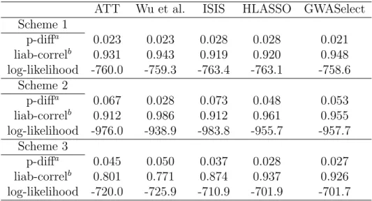
Table 2.2: Prediction accuracy of variable selection methods when the model sizes are fixed at 15 (except for the ATT method)

ATT Wu et al. ISIS HLASSO GWASelect Scheme 1

p-diffa _0.023 _0.023 _0.028 _0.028 _0.021

liab-correlb _0.931 _0.943 _0.919 _0.920 _0.948 log-likelihood -760.0 -759.3 -763.4 -763.1 -758.6

Scheme 2

p-diffa 0.067 0.028 0.073 0.048 0.053

Scheme 3

p-diffa _0.045 _0.050 _0.037 _0.028 _0.027

liab-correlb 0.801 0.771 0.874 0.937 0.926 log-likelihood -720.0 -725.9 -710.9 -701.9 -701.7

a. The absolute difference between the model-predicted and true disease probabilities

(47)

The Wu et al. method excels under scheme 2, consistent with its high TDR and low FDR under this scheme. However, both the Wu et al. and the ATT are less accurate than the other methods under scheme 3 because they missed those marginally uncorrelated SNPs. The HLASSO performs well under scheme 2 and 3, suggesting that high prediction power can be achieved even if some noise features are included in the model. Overall, only the HLASSO and the GWASelect have prediction accuracy above 90% under all three schemes.

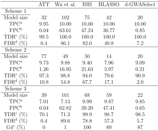
To assess data-adaptive choice of model size, we repeated the above simulation stud-ies but now incorporated a 5-fold cross-validation into all the methods (except the ATT) by using the 10%-error-rate as the evaluation criterion (see Methods) For d-GWASelect, we set the selection threshold ξ to 0.3. All effect sizes were set to be moderate. For both schemes 1 and 3, β∗ = (0.4, −0.4,−0.4,0.4,0.5,−0.5,0.5,−0.6,0.6,−0.6)T_{. For} scheme 2, β∗ = (0.2,0.2,0.2,0.2,0.2,0.2,0.2,0.2,0.2,0.2)T_{. The results are shown in} Tables 2.3 and 2.4.

(48)

Table 2.3: True and false discovery rates when cross validation is incorporated into variable selection (except for the ATT method)

ATT Wu et al. ISIS HLASSO d-GWASelect Scheme 1

Model size 32 102 75 42 20

TPCa _9.95 _10.00 _10.00 _10.00 _10.00

FPCb _0.04 _63.61 _47.24 _30.77 _0.85

TDRc (%) 99.5 100.0 100.0 100.0 100.0

FDRd _(%) _0.4 _86.1 _82.0 _40.8 _7.2

Scheme 2

Model size 77 49 50 14 20

TPCa _9.73 _9.88 _9.40 _7.96 _9.09

FPCb 1.26 16.95 21.63 5.97 0.21

TDRc _(%) _97.3 _98.8 _94.0 _79.6 _90.9

FDRd _(%) _10.8 _54.8 _67.7 _17.1 _2.0

Scheme 3

Model size 39 101 68 59 22

TPCa 7.01 7.13 9.99 9.87 9.85

FPCb _0.04 _62.82 _39.20 _47.41 _0.65

TDRc _(%) _70.1 _71.3 _99.9 _98.7 _98.5

FDRd (%) 0.4 89.6 78.8 57.3 5.7

G4e _(%) ₀ ₁ ₁₀₀ ₈₉ ₈₇

a. Number of true positive clusters b. Number of false positive clusters c. True discovery rate

d. False discovery rate

(49)

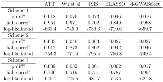
Table 2.4: Prediction accuracy of variable selection methods with cross-validation in-corporated (except for the ATT method)

ATT Wu et al. ISIS HLASSO d-GWASelect Scheme 1

p-diffa _0.018 _0.076 _0.073 _0.046 _0.016

liab-correlb 0.951 0.671 0.702 0.849 0.968 log-likelihood -661.4 -745.9 -739.3 -719.6 -659.7

Scheme 2

p-diffa _0.033 _0.046 _0.063 _0.027 _0.027

Scheme 3

p-diffa 0.039 0.082 0.061 0.062 0.017

liab-correlb _0.786 _0.519 _0.751 _0.787 _0.964 log-likelihood -645.1 -725.5 -681.7 -713.7 -624.8 a. The absolute difference between the model-predicted and true disease probabilities

(50)

2.4 Analysis of WTCCC Data

The WTCCC study examined approximately 2,000 subjects for each of seven com-mon diseases and a shared set of approximately 3,000 controls. Each subject was geno-typed on the Affymetrix GeneChip 500K Mapping Array Set. We provide detailed anal-ysis for the data on Type II diabetes (T2D [MIM 125853, http://www.ncbi.nlm.nih.gov/ omim]) and Type I diabetes (T1D [MIM 222100]), and the analysis for some of the other five diseases is presented in Supplementary Tables 2.10-2.11.

We excluded a small number of subjects according to the sample exclusion lists provided by the WTCCC. In addition, we excluded a SNP if 1) it is on the SNP exclusion list provided by the WTCCC; 2) it has a poor cluster plot as defined by the WTCCC; 3) its MAF<0.01 in both cases and controls; or 4) it has extreme departure from Hardy-Weinberg equilibrium (p-value<10−4). Approximately 390,000 SNPs were used in the analysis, and there were 2,938 controls, 1,924 T2D cases and 1,963 T1D cases.

Figure 2.2 indicates the SNPs selected by the ATT, Wu et al., HLASSO and GWAS-elect for T2D; the details are shown in Table 2.5 and Supplementary Table 2.13. Under the ATT method, 15 SNPs reach the genomewide significance of p-value <10−7. The most significant one is rs4506565 (p-value= 7.5× 10−13), which is located in gene TCF7L2. The other 14 SNPs are clustered within either TCF7L2 or FTO. These re-sults are consistent with the WTCCC’s findings. The HLASSO model is essentially identical to the ATT model, albeit with a smaller model size.

(51)

50 200 chr2

chr1

15 chr6

160 170 180

chr4

170 130

chr5

120 chr position

25 100 110

40 chr10

50 110 120 75 chr12

65

chr15

70 80 5

chr16

15 50 60

15 chr18

5 45

chr21

35 70

60

30 chr7

15

d-GWASelect

Wu et al

ATT HLASSO

Figure 2.2: The T2D models selected by four different methods.

the ATT method.

It is interesting to compare the GWASelect and Wu et al. models. Five SNPs, rs11688935, rs6846031, rs6872465, rs2389591 and rs10435018, show up only in the GWASelect model. Among these SNPs, rs6846031 was selected partly due to its con-ditional correlation with T2D, underscoring the importance of concon-ditional screening in variable selection. This finding also indicates that genetic factors underlying T2D are not simply in parallel with each other, but rather form a complex structure that needs to be carefully dissected.

(52)

T2D. Some of them are plausibly related to T2D. For example, GULP1 is an adaptor protein that binds and directs the trafficking of LRP1 (Su et al., 2002), a protein that has been shown to play a critical role in adipocyte energy homeostasis and insulin sensitivity (Hofmann et al., 2007). Thus, genetic variants in GULP1 may potentially influence the amount of LRP1 in adipocyte cells and thereby modulate a person’s risk to T2D. As another example, the CREB5 was recently found to be down-regulated along with other members of the insulin signaling cascade when stimulated by a ligand of PPARγ, which is known to be associated with T2D (Herrmann et al., 2009). This suggests that CREB5 is closely related to PPARγ and the insulin pathway. The other SNPs do not have known connections with T2D, but further investigation of those loci may reveal novel mechanisms or pathways related to T2D.

For prediction of T2D, the δ-error-rates (with δ=0.1) of all four models are over 40%, suggesting that T2D is greatly influenced by other types of genetic variations and environmental factors. Since it is not very meaningful to compare prediction errors at such high level, we turned our attention to the T1D data because it is well-known that T1D is genetically more homogeneous than T2D.

(53)

Table 2.5: List of SNPs selected by the GWASelect for the WTCCC-T2D

SNPa _Chromosome _Geneb

rs11688935 2 GULP1

rs903228 2 ASB3/LOC129656

rs6846031 4 VEGFC/NEIL3

rs6872465 5 PRDM6

rs10806665 6 THBS2/SMOC2

rs9465871 6 CDKAL1

rs2389591 7 TMEM195/LOC729920

rs10435018 7 CREB5

rs7917983 10 TCF7L2

rs7901695 10 TCF7L2

rs4506565 10 TCF7L2

rs4132670 10 TCF7L2

rs7077039 10 TCF7L2

rs9326506 10 ZNF239

rs1495377 12 TSPAN8/LGR5

rs7961581 12 TSPAN8/LGR5

rs2930291 15 CCDC33

rs8050136 16 FTO

rs2099106 16 C16orf72/GRIN2A

rs6517434 21 KCNJ6

a. rs number identified from dbSNP

(54)

expression ofNeuroD (Lulianella et al., 2008), a gene that can cause T1D if mutated. Finally, we compared the prediction accuracy of the four methods. We randomly divided the data into three parts, two as the training data and one as the testing data. Since the training data set contains only 2/3 of the original data, we reduced ξ from 0.20 to 0.10 to ensure that a similar number of loci are included in the d-GWASelect model. Since the true liability scores and disease probabilities are unknown in real data, we measured the prediction errors by theδ-error-rates forδ = 0.1, 0.15 and 0.25 (see Methods for detail). Considering that pruning was done before each model was used for prediction, we report the actual (i.e., effective) number of SNPs used by each model for prediction. Under default settings, the effective model sizes of the Wu et al., the HLASSO and the d-GWASelect are 14, 4 and 21, respectively. Since the former two models are much smaller, we also evaluated the prediction accuracy of the former two under 21 effective SNPs. (We were not able to evaluate the ATT under 21 effective SNPs due to numerical instabilities.) The results are reported in Table 2.7. Clearly, the d-GWASelect performs the best or nearly the best for all threeδ-error-rates. We have also calculated the area under the ROC curve for the four methods, and GWASelect achieves the highest value (Supplementary Table 2.15).

2.5 Discussion

(55)

Table 2.6: List of SNPs selected by the d-GWASelect for the WTCCC-T1D

SNPa _Chromosome _Geneb

rs6679677 1 RSBN1/PTPN22

rs41515647 1 ST6GALNAC5

rs17388568 4 ADAD1

rs330483 4 ADAM29

rs9273363 6 HLA-DQB1

rs9272346 6 HLA-DQA1

rs411136 6 SYNGAP1

rs1265566 12 CUX2

rs7398833 12 CUX2

rs10744777 12 ALDH2

rs17696736 12 C12orf30

rs11171739 12 ERBB3

rs12708716 16 CLEC16A

rs12924729 16 CLEC16A

a. rs number identified from dbSNP

b. Gene symbol from Entrez Gene

Table 2.7: Prediction errors for the WTCCC-T1D

model effective δ-error-rate

log-size 0.1 0.15 0.25 likelihood

ATT 5 0.110 0.139 0.181 -2116.9

Wu et al. 14 0.119 0.139 0.179 -2075.1 21 0.135 0.157 0.196 -2059.8

HLASSO 4 0.116 0.141 0.176 -2113.6

(56)

60 120 chr1

210 chr2

120 170

chr4

32 34

chr6

200

50 chr12

40 chr5

30

60 110.2 111.0 40 chr10

30

50 chr14

40

40 chr17

30 20

chr18

10 20 chr16

10

d-GWASelect

Wu et al

ATT chr position

HLASSO

(57)

not require the specification of the model size, and this is the version we recommend for general use.

The correlation structures for causal variants used in our simulation studies have biological relevance. Scheme 2 mimics a scenario in which the causal variants form a gene cluster that contributes synergistically to the disease outcome, while scheme 3 reflects a scenario in which several biological pathways (or networks) affect the disease development.

We did not include Least Angle Regression (LARS) in our studies because it has been shown to have highly similar performance to LASSO (Hastie et al., 2009). Indeed, LASSO can be implemented by LARS with a small modification. Wu and Lange (2008) demonstrated that CCD is “considerably faster and more robust than LARS” and is “more successful than LARS in model selection”.

The HLASSO adopts a concave penalty function, and it has been suggested that the CCD algorithm may not converge for nonconvex penalty (Wu et al., 2009; Friedman et al., 2010). A valid algorithm to implement concave penalty functions is the local linear approximation (Zou and Li, 2008), which amounts to multiple rounds of CCD and would make the HLASSO computation prohibitively expensive. For the WTCCC T1D data, running the CCD version of the HLASSO with 10 iterations on an Intel Quadcore Nehalem processor (2.4Ghz, 16GB memory) require 67.5 to 175 hours, depending on the value of the tuning parameter. In contrast, we have been running the GWASelect in a parallel computing environment, and the same analysis can be completed within several hours on 16 processors.

(58)

method tends to have high FDR. They observed that cross-validation tends to yield large models for logistic regression, resonating our findings in the Simulation Studies.

We can extend our methods to select interactions. Instead of considering all possible interaction terms, we may incorporate known biological network information (Franke et al., 2006) into our selection procedure. Another approach is to first extend the existing genetic network identification tools, such as the liquid association (Li, 2002) and bounded mode stochastic search (Dobra, 2007), to infer SNP interactions and then incorporate such information into our GWASelect procedure. In fact, Han et al. (2010) proposed a Markov blanket-based method to evaluate epistatic interactions for GWAS data. It will be interesting to compare to that method when we extend our work to interaction effects.

How to obtain p-values for high-dimensional variable selection is an active research area. The stochastic error introduced by the selection process makes it very difficult to assign p-values to the selected features. Meinshausen et al. (2009) offered one possible solution by “aggregating”p-values from stability selection, but our experiments indicated that this procedure is too conservative for SNP data, likely due to the ultra-high dimension and strong LD. We hope future progress will shed light on this important issue.