The oldest and most metal-poor stars in the APOSTLE Local Group
simulations
Else Starkenburg,
1‹Kyle A. Oman,
2Julio F. Navarro,
2Robert A. Crain,
3†
Azadeh Fattahi,
2Carlos S. Frenk,
4Till Sawala
5and Joop Schaye
61Leibniz Institute for Astrophysics Potsdam (AIP), An der Sternwarte 16, D-14482 Potsdam, Germany
2Department of Physics and Astronomy, University of Victoria, PO Box 3055, STN CSC, Victoria, BC V8W 3P6, Canada
3Astrophysics Research Institute, Liverpool John Moores University, IC2, Liverpool Science Park, 146 Brownlow Hill, Liverpool L3 5RF, UK
4Institute for Computational Cosmology, Durham University, South Road, Durham, DH1, 3LE, UK
5Department of Physics, University of Helsinki, Gustaf H¨allstr¨omin katu 2a, FI-00560 Helsinki, Finland
6Leiden Observatory, Leiden University, PO Box 9513, NL-2300 RA Leiden, the Netherlands
Accepted 2016 November 4. Received 2016 November 3; in original form 2016 July 4
A B S T R A C T
We examine the spatial distribution of the oldest and most metal-poor stellar populations of Milky Way-sized galaxies using the A Project Of Simulating The Local Environment (APOSTLE) cosmological hydrodynamical simulations of the Local Group. In agreement with earlier work, we find strong radial gradients in the fraction of the oldest (tform<0.8 Gyr) and most metal-poor ([Fe/H]<−2.5) stars, both of which increase outwards. The most metal-poor stars form over an extended period of time; half of them form afterz=5.3, and the last 10 per cent afterz=2.8. The age of the metal-poor stellar population also shows significant variation with environment; a high fraction of them are old in the galaxy’s central regions and an even higher fraction in some individual dwarf galaxies, with substantial scatter from dwarf to dwarf. We investigate the dependence of these results on the assumptions made for metal mixing. Overall, over half of the stars that belong to both the oldest and most metal-poor population are found outside the solar circle. Somewhat counter-intuitively, we find that dwarf galaxies with a large fraction of poor stars that are very old are systems where metal-poor stars are relatively rare, but where a substantial old population is present. Our results provide guidance for interpreting the results of surveys designed to hunt for the earliest and most pristine stellar component of our Milky Way.
Key words: stars: abundances – Galaxy: formation – galaxies: dwarf – Local Group – dark ages, reionization, first stars – early Universe.
1 I N T R O D U C T I O N
It is often assumed that the most metal-poor stars today are the oldest objects in the Galaxy and as such they are the most extensively studied relics from the ancient Universe. While very useful as a first-order approximation, it is nevertheless obvious that the adoption of metallicity as a clock is valid only in closed-box environments, where metals are well mixed at all times. In reality, it is expected that chemical evolution starts and progresses at different rates in various environments. To complicate matters even more, theCDM cosmological paradigm of hierarchical formation allows stars to find themselves in very different environments throughout their lives – albeit still bearing the chemical imprint of their birth location.
E-mail:estarkenburg@aip.de
†Royal Society University Research Fellow.
The very first stars in the Universe are expected to form in en-vironments that are overdense at early times. In low-density envi-ronments on the other hand, pristine stars may have formed much later provided that the gas in them has remained unpolluted. Simu-lations suggest that pristine stars can still form at moderate redshifts well after the completion of global reionization (e.g. Scannapieco, Schneider & Ferrara2003; Scannapieco et al.2006; Tornatore, Fer-rara & Schneider2007; Trenti, Stiavelli & Michael Shull 2009; Muratov et al.2013b; Salvadori et al.2014; Xu et al.2016). A dis-tinction is sometimes made between those stars that were formed out of unpolluted gas but have been affected by radiation or kine-matical feedback from other nearby stars, and those that are truly the first stars in their environment (e.g. McKee & Tan2008).
it is unclear at what level later fragmentation of the protostellar cloud could facilitate the formation of subsolar mass stars which – even if formed at the dawn of time – would still be around to-day (see Bromm2013; Karlsson, Bromm & Bland-Hawthorn2013; Greif2015, and references therein). Furthermore, a full treatment of metal-line, molecular, and dust cooling, stellar nucleosynthesis of zero-metallicity stars, their stellar feedback and the reioniza-tion epoch would be needed to model accurately the epoch of the first stars. None of these processes are well understood and even when certain assumptions are made, it is particularly challenging and computationally expensive to simulate them within a fully cos-mological setting. Modelling studies have therefore predominantly either focused on a detailed treatment of processes in the early uni-verse in a limited volume and/or a limited time (e.g. Abel, Bryan & Norman2002; Wise et al. 2012; Muratov et al. 2013a,b; Smith et al.2015), or resorted to a simpler treatment of physical processes – often through a so-called semi-analytical approach whereby physi-cal processes are modelled by analytiphysi-cal relations on top of a cosmo-logical merger tree or Press–Schechter formalism (e.g. Scannapieco et al.2003,2006; Yoshida, Bromm & Hernquist2004; Salvadori, Schneider & Ferrara2007; Gao et al.2010; Komiya et al.2010; Salvadori et al.2010; Tumlinson2010; Hartwig et al.2015).
Observational endeavours have been extremely helpful in con-straining models of early epoch star formation in the Milky Way. Several survey efforts have been mining the Milky Way stars for the lowest metallicity members (e.g. Beers, Preston & Shectman1985; Christlieb2003; Keller et al.2007; Schlaufman & Casey 2014; Casey & Schlaufman2015; Howes et al.2016), and in the com-ing decade it is expected that the search for metal-poor stars will intensify. At present, nine stars are known to have [Fe/H]<−4.5 (Christlieb, Wisotzki & Graßhoff2002; Frebel et al.2005,2015; Norris et al.2007; Caffau et al.2011; Hansen et al.2014; Keller et al.2014; Bonifacio et al.2015). With such low numbers of stars at the lowest metallicities, any history of the Milky Way’s earliest epochs that might be derived from them would remain anecdotal at best. Another limitation of observational work in this field is that age determinations of individual stars have large uncertainties, up to several gigayears for old ages.
The best avenue available to link these stars to the very early Universe is by comparing their abundance patterns to the predicted yields for metal-free massive stars. For instance, the most iron-poor star, SMSS J031300.36−670839.3 at [Fe/H]<−7.0 could be linked to an∼60 solar-mass, zero-metallicity progenitor (Keller et al.2014). It is particularly intriguing that, from analysis of the limited numbers of extremely metal-poor stars ([Fe/H]<−3), it seems that their abundance patterns vary with environment in the Galaxy. Recently, Howes et al. (2015) showed that in 23 stars in the bulge region none shows significant carbon enhancement, whereas this occurs in∼32 per cent of halo stars of such low metallicities (Yong et al.2013). Although always based on small samples, in earlier work it has already been noticed that the number of carbon-enhanced stars (or their abundance patterns) seems to change as a function of environment. Variations – or hints thereof – have been reported with increasing disc height (Frebel et al.2006), in the inner versus outer halo (Carollo et al.2014) and in the Sculp-tor dwarf spheroidal galaxy compared to the halo (Starkenburg et al.2013; Sk´ulad´ottir et al.2015). If confirmed by larger stud-ies, this might indicate that the most metal-poor stars in various Milky Way environments have been formed through different chan-nels, or even at different times (see also the discussion in Gilmore et al.2013; Norris et al.2013; Starkenburg et al.2014; Salvadori, Sk´ulad´ottir & Tolstoy2015).
Similarly, the diversity in abundance patterns found among the metal-poor stars in satellite galaxies can give us also clues on the early Universe and chemical enrichment processes (one of the more striking examples are the r-process enhanced stars in Reticulum II; Ji et al.2016). Observationally, dwarf galaxies – and particularly those as close to us as the satellites of the Milky Way – are of great value, because they allow us to study in detail the early formation of galaxies in a different mass scale. Some of the faintest systems, be-longing to the class of so-called ultrafaint galaxies, seem to qualify to be ‘first galaxies’ or ‘fossil galaxies’ – meaning that the great ma-jority of their total stellar population was formed before the epoch of reionization (Bovill & Ricotti2009,2011a,b). However, which and how many systems exactly qualify fossil galaxies criteria are debated and it is unclear to what extent quenching through tidal disturbance by the Milky Way could influence these results (Weisz et al.2014). Brown et al. (2014) derive ages fromHubble Space Telescopecolour–magnitude diagrams for six ultrafaint galaxies and find that all of them are consistent with having formed 80 per cent of their stars byz=6. Additional evidence for only one short burst of star formation can come from chemical element analysis of their stars showing no enrichment by, for instance, supernovae Type Ia products or s-process elements (Frebel & Bromm 2012; Frebel, Simon & Kirby2014).
In this work, we study the early generations of stars in the A Project Of Simulating The Local Environment (APOSTLE) sim-ulations (Fattahi et al.2016; Sawala et al.2016). This is a suite of 12 volumes selected to resemble the Local Group simulated with sufficient mass resolution to study the Milky Way and Andromeda-type galaxies as well as their smaller companions and isolated dwarf systems. Moreover, the hydrodynamical nature of the simulations allows us to follow enrichment and feedback processes more self-consistently than in semi-analytic frameworks. The main purpose of this work is to present further predictions and guidelines for the interpretation of present and future surveys of metal-poor stars throughout the Galaxy. We will introduce our suite of simulations in more detail in Section 2. We first review the general distribution of metallicity and age within the Milky Way and M31 analogues in Section 3.1, before focusing our attention on the oldest and most metal-poor stars in Sections 3 and 4, where we study their distribu-tion in the main galaxies. Addidistribu-tionally, we compare these findings with the old and most metal-poor populations in the surviving satel-lites and isolated dwarf galaxies in Section 5. To aid future surveys, we discuss how to find the systems in which a metal-poor star is most likely to be very old in Section 5.1. We finally discuss the assumptions and a comparison with literature results in Section 6. Throughout this paper, we adopt the solar abundance for iron to be logFe=7.501(Asplund et al.2009).
2 T H E A P O S T L E S I M U L AT I O N S
The APOSTLE simulations are described in detail by Sawala et al. (2016) and Fattahi et al. (2016). In brief, the APOSTLE set consists of 12 halo pairs that are selected from the larger cosmological DOVE simulation volume (Jenkins2013) and resemble the Local Group pair of galaxies in several properties: (i) their spatial separation (between 600 and 1000 kpc), (ii) their relative radial velocity (in the range−250 to 0 km s−1), (iii) their relative tangential velocity
(less than 100 km s−1), (iv) their total pair mass (log
10(Mtot/M) is
between 12.2 and 12.62) and (v) they are sufficiently isolated, with
no haloes larger than the smallest of the pair within 2.5 Mpc of the mid-point of the pair and a relatively unperturbed Hubble flow out to 4 Mpc. Interestingly, Fattahi et al. (2016) find that halo pairs that satisfy these criteria are on average a factor of 2 lighter than the total mass of the Local Group estimated from the timing argument. The median masses of the primary and secondary haloes in each region are 1.4×10¹²M
and 0.9×10¹²M
, respectively. Each region samples a high-resolution sphere out to at least 2.5 Mpc, so many more nearby isolated systems within the Local Volume can also be studied. The APOSTLE simulations are run at three resolution levels labelled ‘L1’, ‘L2’ and ‘L3’ and have approximate dark matter particle masses of 5.0 ×10⁴, 5.9 ×10⁵ and 7.5×
106M
, and approximate primordial gas particle masses of 1.0× 10⁴, 1.2×10⁵and 1.5×10⁶M
, respectively. Only AP-1, AP-4 and AP-11 have been simulated at the highest (L1) resolution. The simulations at resolutions L2 and L3 have been completed for all 12 volumes. The different resolutions use identical subgrid models and parameter values. Our adopted cosmology is that ofWMAP-7 (Komatsu et al.2011).
Although performed at sufficiently high resolution to be able to resolve small substructure such as satellite dwarf galaxies, the res-olution is not sufficient to resolve individual star formation regions or supernova events. These physical processes are governed by the well-calibrated and well-tested physics model used for the EAGLE project (Crain et al.2015; Schaye et al.2015). Our implementation uses the parameter values from the L100N1504 reference simulation presented by Schaye et al. (2015). The star formation is modelled to follow the Kennicut–Schmidt star formation law. The rate of star formation is calculated depending on pressure rather than (more commonly used) volume density (Schaye & Dalla Vecchia2008) with a metallicity-dependent density threshold (Schaye2004). Stel-lar thermal feedback is modelled as presented by Dalla Vecchia & Schaye (2012). Reionization (of hydrogen) is modelled to be instan-taneous atz=11.5 following the prescriptions of Haardt & Madau (2012) and Wiersma, Schaye & Smith (2009a).
The stellar evolution feedback processes responsible for chemi-cal enrichment include winds from Asymptotic giant branch (AGB) stars, Type Ia supernovae, Type II supernovae and winds from their progenitors (for details see the descriptions in Wiersma et al.2009b). The supernova Ia rates from Schaye et al. (2015) are shown to be in broad agreement with the observed evolution of the supernova Ia rate density. Yields are taken from Portinari, Chiosi & Bressan (1998), Marigo (2001) and Thielemann et al. (2003). Each star par-ticle is treated as a simple stellar population with a Chabrier IMF (Chabrier2003). Finite stellar lifetimes are implemented that are metallicity dependent (Portinari et al.1998). Stellar mass loss is distributed over 48 neighbouring particles using a smoothed par-ticle hydrodynamics (SPH) kernel transport scheme (Pawlik & Schaye2008), after setting the mass of the gas particles equal to a constant initial value (Schaye et al.2015). 11 different elements are followed throughout the simulation: H, He, C, N, O, Ne, Mg, Si, S, Ca and Fe. The same elements are used to calculate radiative cooling.
No special treatment of the first stellar generation is implemented in our APOSTLE simulations; the first stars forming in the simu-lation are modelled with an identical IMF and supernovae feed-back as later generations. However, even if the first stars should
2When quoting halo masses, we useM200, the mass enclosed within a spher-ical volume where the mean overdensity is 200 times the critspher-ical density.
be very peculiar in their properties, star formation processes will generally normalize in a few generations when metals become avail-able. We will therefore focus on the first generations of stars that were formed, rather than the very first stars themselves.
3 T H E O L D E S T A N D M O S T M E TA L - P O O R S TA R S
In this work, we focus on the most metal-poor and oldest generations of stars and their distribution in the simulations. We define ‘oldest’ and ‘most metal-poor’ as follows for the remainder of the paper:
(i)oldest: formation time<0.8 Gyr after the big bang (i.e. redshift >6.9);
(ii) most metal-poor: [Fe/H]<−2.5.
These choices are naturally somewhat arbitrary, but nevertheless motivated by the results from observational surveys that tend to provide spectroscopic results for stars in the low-metallicity regime from [Fe/H]= −2.5 and below. The age restriction is motivated by the approximate time-scale for reionization. A time of 0.8 Gyr after the big bang corresponds to a redshift ofz=6.9, close to the epoch of reionization.3We want to refrain from making the age cut
too close to the big bang itself, because as motivated already in the Introduction section, we have no firm knowledge of the formation of the very first stars and no special modelling of these is provided in our simulations. We therefore believe our results will be more robust when the focus lies on the first several generations rather than the very first alone. An additional advantage of the cuts made is that the numbers of most metal-poor stars and the numbers of oldest stars according to these criteria are roughly equal. We refer the reader to Section 6 for a discussion on the robustness of our results regarding these choices.
3.1 Metallicity and age distributions in the APOSTLE galaxies
Before directing our attention fully to the oldest and most metal-poor stars, we first investigate the overall metallicity and age profiles of the APOSTLE main haloes in order to understand the main prop-erties of the galaxies we study in this work. Open histograms in Fig.1show the stacked age and metallicity distribution functions of the main galaxies (primary and secondary haloes of each pair) within the APOSTLE simulations for all intermediate resolution L2 runs – these are available for all 12 volumes. In this analysis, we in-clude any bound substructures that have survived in the main haloes. We represent metallicity by [Fe/H], as is common in observational studies.4Additionally, we have chosen to use the SPH-smoothed
metallicity values. As described in section 5.2 of Wiersma et al.
(2009b), the smoothed metallicity formalism – in which the
metal-licity of a star is set at its time of formation as the ratio of the SPH-smoothed gas metal mass density and the SPH-smoothed gas mass density – has the advantage that it is better tailored to the na-ture of SPH simulations and furthermore that it somewhat alleviates the absence of a metal mixing formalism in the code. The smoothed abundances were also used in the simulations themselves for the calculation of cooling rates, stellar yields and stellar lifetimes.
3In our simulations, reionization is forced to externally occur atz=11.5; this corresponds to 0.4 Gyr after the big bang.
4In this notation, [Fe/H]=log 10
NFe
NH
stars−log10
NFe
NH
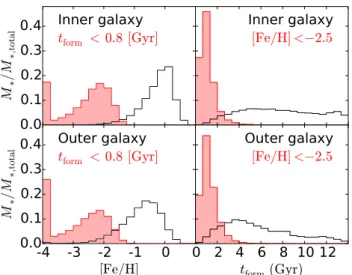
Figure 1. Metallicity and age distribution functions for all APOSTLE main galaxies (resembling the MW and/or M31 in mass) in all intermediate resolution L2 runs. We represent either the inner regions of the galaxies (r<15 kpc) or their outer halo populations (15<r<100 kpc), where for the latter we have left anyin situpopulations out (see the text for details). The open black histograms represent the full sample of all stellar particles within these radial cuts. The red-shaded histograms represent a subset of the oldest stars (in the two left-hand panels; formation time<0.8 Gyr after the big bang) or the most metal-poor stars (the two right-hand panels; [Fe/H]<
−2.5) for the same radial selections. Both the open and shaded histograms are normalized to the total mass in stars in their sample, the red-shaded histograms contain in all cases less than 2 per cent of the stars in the open black histograms. Stars with metallicities less than−4 are shown in the lowest metallicity bin.
In Fig. 1, a rough distinction is made between the inner and outer galaxy components, to be within or outside a radius of 15 kpc from the galaxy’s centre, respectively (and within 100 kpc). SPH, in combination with subgrid star formation prescriptions, are known to be sensitive to the precise treatment of thermal instabilities and can sometimes form stars in unstable pockets of (initially hot) halo gas in larger galaxies (e.g. Kaufmann et al.2006; Kereˇs et al.2012; Parry et al.2012; Hobbs et al.2013; Cooper et al.2015). Although the severity of this problem is greatly reduced in EAGLE by the use of the ‘Anarchy’ hydrodynamics solver (Schaller et al.2015), we avoid any influence of these numerical ‘nuisance’ events on our results, by showing in the panels for stars at distances>15 kpc only stars that have not formed ‘in situ’ in the halo of the main galaxy. In practice, this means that the outer galaxy includes only the ‘accreted’ component of the stellar halo, as well as other bound substructures.
While the build-up of the inner galaxy as well as the halo metal-licity distribution function over cosmic time is interesting in its own right, we leave this as a topic for future work; for the purposes of this paper, it is mainly interesting to note that there is a difference between both populations in terms of ages and metallicities. In the outer regions beyond 15 kpc, these galaxies have a peak at earlier formation time (∼3 Gyr) and lower metallicities ([Fe/H]≈ −0.6). Additionally, for the outer components, the tail of the metallicity distribution extends to lower metallicity. Qualitatively, this agrees with observational evidence in the Milky Way, where we also see that the outer halo contains a much larger fraction of old, metal-poor and very metal-metal-poor stars when compared to the more central regions (e.g. Helmi2008; Bland-Hawthorn & Gerhard2016). How-ever, the peak metallicity of the Milky Way halo population is at a
lower value. Allende Prieto et al. (2014) find that for their sample of tens of thousands of turn-off stars withg-band magnitude>17 and distances ranging from five to tens of kiloparsecs from the Sun, the peak of the metallicity distribution is at [Fe/H]= −1.6, dropping to [Fe/H]≈ −2.2 for stars beyond 10 kpc from the Sun [these values are in good agreement with previous work (Carollo et al.2007,2010; de Jong et al.2010; Beers et al.2012)]. Although we do see some individual galaxies in the simulation with a lower metallicity peak in the outer galaxy, our mass-averaged main Local Group galaxies as shown here bear more resemblance to observations in M31 (e.g. Durrell, Harris & Pritchet2004; Gilbert et al.2014) where a halo population peaking at [Fe/H]∼ −0.5 is seen (even at a radius of 30 kpc or beyond), with a long tail towards low metallicities.
As illustrated in the shaded histograms in Fig.1, the oldest stars in a galaxy tend to be more metal poor than the average and vice versa – the most metal-poor stars in a galaxy are older on average. However, within these shaded histograms there is clearly still a large range. Not all stars that are older than 0.8 Gyr are very metal poor (indeed, the population reaches its peak a bit below [Fe/H]= −2) and using our most metal-poor cut, we select stars with a range of ages up to several Gyr after the big bang. We find that 50 per cent of the most metal-poor stars form within 1.1 Gyr and 90 per cent within 2.4 Gyr (corresponding toz=5.3 and 2.8, respectively).
4 A R E T H E M O S T M E TA L - P O O R S TA R S A L S O O L D ?
In the previous section, we have investigated the oldest and most metal-poor stars in the simulations; here we combine the two criteria and ask: if we observe a metal-poor star in any particular environ-ment, will it also be old? In other words: where will the first-order approximation best hold that the most metal-poor stars are messen-gers from the early Universe? This question is particularly relevant for observational surveys aiming to find metal-poor stars and mea-sure their metallicity, but that are unable to meamea-sure their precise ages.
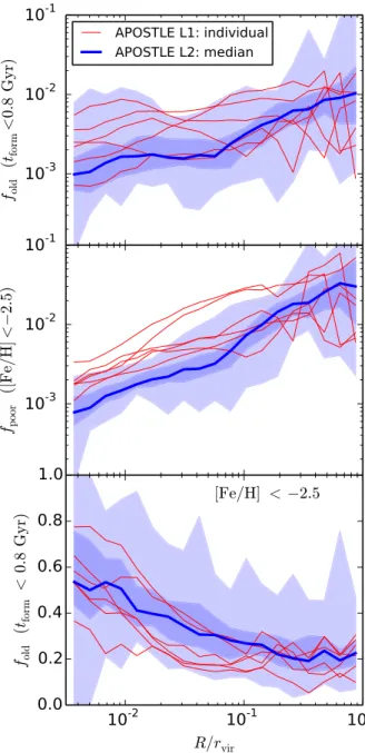
The top and middle panels of Fig.2show the fraction of oldest and the fraction of most metal-poor stars as a function of radius in each of the main galaxies out to their virial radius. The fraction of both old and most metal-poor stars increases in the outskirts of these galaxies, suggesting that a perfect place to look for either of these populations would be the Galactic halo. The bottom panel of Fig.2shows the radial profile within the main galaxies, similarly to the top panels, but now for the most metal-poor stars that are also old. We see that the trend is the reverse from that shown in the top two panels. When a star is selected that is metal poor (as one would in an observational study), the probability that the star is old is lower in the galaxy out-skirts than in the centre. This general trend of finding the oldest stars (among the metal-poor stars) mainly in the centre of the galaxy has been discussed before (White & Springel2000; Brook et al.2007; Gao et al.2010; Salvadori et al.2010; Tumlinson2010; Ishiyama et al.2016) and is generally explained by the first stars forming in the density peaks that collapse first in the universe, these then generally end up in the centres of the main haloes. However, quanti-tatively the results of the various studies vary significantly, reflecting uncertainties in the modelling of early universe physics. We refer the reader to the discussion in Section 6 for a more detailed and quantitative comparison of earlier work with our results.
Figure 2. Top and middle panels: the fraction of oldest and the fraction of most metal-poor stars, respectively, as a function of radius in each of the main galaxies out to their virial radius. For the L2 simulations, a median curve of all main galaxies is shown, whereas the six main galaxies simulated at higher resolution, L1, are shown as individual (red) lines. Blue-shaded regions show the interquartile and full range of the L2 simulations. Bottom panel: the fraction of most metal-poor stars that are old (see the text for definitions).
most of the individual L1 runs deviate somewhat from the median result for all L2 galaxies (most notably in the middle panel). In Fig.A1in Appendix A, we demonstrate further that the populations we focus on are only weakly affected by resolution effects, at least when comparing the L1 and L2 runs. We will therefore focus on these resolutions for the remainder of the paper.
We additionally note that our results are virtually insensitive to the inclusion or exclusion of the possibly spuriousin situouter halo star population discussed in Section 3.1. While the fractions of old ormetal-poor populations shown in the top panels of Fig.2show an increase when only accreted stars are considered, there is very
little difference in the ratio of most metal-poor stars that are old, as defined in the bottom panel. The reason is thatin situstars form later and out of metal-enriched gas. Hence they increase the total population of stars, but do not affect the populations of interest in this paper.
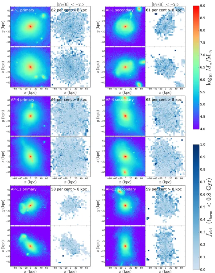
Following up on the general trend of more centrally concentrated oldandmetal-poor populations, we explore the spatial distribution of the most metal-poor populations in the galaxies in more detail in Fig.3. Shown here are two orthogonal projections of all stars within a 300 kpc radius of each of the six main galaxies in the three highest resolution L1 APOSTLE simulations. The left-hand panels of each grid show a logarithmic colour-coded stellar mass map of the galaxy out to 75 kpc from the galaxy centre. The right-hand panels of each subplot show only those stars that are most metal poor according to our criterion in each spatial bin (the bin size is allowed to vary according to the density of stellar populations in that area), and the colour coding is chosen so that it follows the fraction of the most metal-poor stars that are old within this population. Several striking features stand out from these figures.
(i) We still see the general trend that the metal-poor population is older at the centre than in the outskirts, as is shown already in Fig.2and can be seen here by a darker shade in the centres of the galaxies in the right-hand panels (most notably visible in AP-1 primary, AP-4 primary and secondary and AP-11 secondary galaxies).
(ii) However, in the outskirts of the galaxies, typically at scales of several tens of kiloparsecseachof our six modelled galaxies shows particularly interesting substructures that are on average very old – frequently even more so than the metal-poor stars in the central few kiloparsecs. The distribution of this population changes from galaxy to galaxy.
(iii) As can be seen from the comparison with visual overdensi-ties, this population is often connected to their individual merging histories. The oldest substructures frequently correspond to bound or disrupting satellites. For instance, all darkest pixels in right-hand panels of the AP-4 secondary galaxy, or AP-11 primary galaxy cor-respond to compact overdensities in the stellar density maps. In the AP-1 secondary galaxy, we see a large satellite galaxy disrupting at (x,y)≈(20, 50). Careful inspection of the stellar density map reveals a bridge of stars connecting it to the main host [from (x,y)
≈(20, 50) to (x,y)≈(−20, 30)]. We observe the same feature in darker shades in the right-hand panel.
(iv) These metal-poor andoldest populations in the halo gen-erally follow substructures, but not all substructures. More im-portantly, they sometimes trace merging events that are not ap-parent in the overall stellar density because the metallicity and age contrast is much greater than the surface density contrast. An example of this can be seen in the secondary halo of AP-1 (top-right panel), where at (x, y) ≈ (0, −55) a very old and metal-poor substructure stands out that is not visible in the full stellar density map.
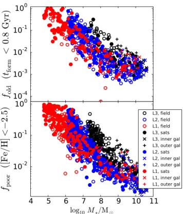
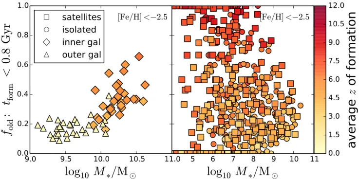
Figure 4. The left-hand panel shows the mass fraction of old stars among the most metal-poor populations shown for the inner and outer galaxy components (defined asr<15 kpc and 15<r<100 kpc, shown as diamonds and triangles, respectively) of each L1 or L2 main galaxy as a function of the total stellar mass at those radii. The right-hand panel shows the same metric, but now for every dwarf galaxy included in the simulation within a 2 Mpc sphere. Satellite systems, within 300 kpc of either one of the main galaxies, are shown as squares, isolated dwarf galaxies as circles. The symbols are colour coded according to the average redshift of formation of their most metal-poor population. The colour gradient that is visible across they-axis of the figure confirms that the metric chosen here (the fraction of most metal-poor stars that are also old, where old means formed before 0.8 Gyr or a redshift of 6.9) is indeed correlated with the average formation time and that no spurious behaviour is introduced by imposing a sharp threshold for what we call ‘old’.
interesting stars are found outside the solar radius than within.5We
verified that this result is robust to the simulation resolution; in the medium resolution L2 galaxies we also find very similar fractions for the most metal-poor and oldest stars outside the solar radius, with a median for all 24 galaxies of 62.2 per cent. Approximately half of the population of most metal-poor and oldest stars is found outside a radius of 14 kpc, indicating that surveys need to reach out quite far to study the full population. To observe the sample to 90 per cent completeness, one has to extend the survey out to
≈95 kpc. The large majority of all most metal-poor and oldest stars are part of the main galaxy (i.e. they do not belong to any bound substructure atz =0), but nevertheless a significant fraction (on average 19 per cent) of them belong to bound substructures. In the next section, we look into the various surviving substructures to see if we can disentangle the systems that stand out in this respect from their peers.
5 C O M PA R I N G T H E H A L O P O P U L AT I O N T O T H E S U RV I V I N G S AT E L L I T E S A N D
I S O L AT E D DWA R F G A L A X I E S
In Fig.4, we investigate the fraction of oldest stars among the most metal-poor stars for galaxies as a whole. In this comparison, we include all galaxies with a stellar mass over 104M
, comparable to the Milky Way satellites Bo¨otes I, Leo IV, or Leo V, which are on
5Naturally, not each of these galaxies represents a Milky Way and the shapes and sizes of their stellar components vary, which means that we are not probing the same mix of stellar components at this fixed radius (Campbell et al.2016).
the brighter end of the so-called ultrafaint galaxies. While we can include also more isolated dwarf galaxies down to this mass limit, these will be typically too faint to be observed; Leo T at a distance of over 400 kpc that has≈1.4×10⁵M
is at the low-luminosity end of the more isolated dwarf galaxies (McConnachie2012, and references therein). Like in observational data, we find that our simulated dwarf galaxies obey a mass–metallicity relation where the fainter galaxies are more metal poor. For a typical dwarf galaxy of 106M
Figure 5. Age–metallicity relations for dwarf galaxies that have a high fraction of oldest stars among their most metal-poor populations (bottom panel) and those that have a low fraction (top panel). The fractions are chosen so that the sum of their stellar masses in both panels is roughly equal. Grey lines indicate the definitions of oldest and most metal poor as defined in Section 3 and used here and throughout this paper.
If we could isolate the oldest stars in these systems, then this would offer great potential for early-universe studies across various environments. However, as the right-hand panel of Fig.4illustrates, any given star of [Fe/H]<−2.5 in a dwarf galaxy system might be a messenger from the distant past, but could also be a much more recently formed object. How can we distinguish between those satellite systems that host stars formed before or during the epoch of reionization and those that don’t?
5.1 How to find the systems where more metal-poor stars are old?
In Fig.5, we analyse the age-[Fe/H] distributions for those dwarf galaxies that have a high fraction of old stars among their most metal-poor populations (in the bottom panel) and those that have a low fraction (in the top panel). It is clear from this figure that the dwarf galaxies with high fractions of old stars among their most metal-poor stars start to form stars earlierandare more effective at enriching themselves; they do not form metal-poor stars anymore at later stages.
It is in the interest of future surveys hunting for old stars to separate the galaxies in the bottom panel of Fig. 5 from those in the top panel. However, it is very challenging observationally to provide the necessary accuracy on the age determination. In general, it is difficult to find any imprints of the very first stages of star formation still in the dwarfs today. For most dwarf galaxies, the overwhelmingly larger more metal-rich and younger populations contain little information on the first stages of star formation – indeed, we found no clues to the value offold in any present-day
observable like star formation history, metallicity distribution or even morphology or compactness of the resulting dwarf galaxy.
One interesting parameter that can be measured, however, even in distant systems, is the fraction of the stellar population older
Figure 6. The fraction of age>10 Gyr populations in dwarf galaxies and the fraction of stars with [Fe/H]<−2.5, colour coded by the fraction of these most metal-poor stars that are old (formed before 0.8 Gyr after the big bang). Squares are satellite galaxies within 300 kpc of their host; circles indicate more isolated systems. The red line indicates a suggested cut in this parameter space (sloping up from<10 to<20 per cent most metal-poor stars of their total stellar population, as a function of the fraction of stars older than 10 Gyr) to select the systems with a high chance of having very old stars amongst their most metal-poor population (see the text for details).
than∼10 Gyr (because this population has specific tracers, i.e. RR-Lyrae stars). In Fig.6, we show how this metric, if combined with a measurement of the (mass-)fraction of the most metal-poor stars, can provide a much more successful identification of dwarf galaxy systems in which to search for very old stars.
Without any pre-selection, we find that in∼18 per cent of the dwarf galaxies observed (both field and satellite galaxies) over 50 per cent of their most metal-poor stars are old. Since these are the systems most interesting for old star search campaigns, we define our blind search ‘success rate’ as 18 per cent. However, if instead of selecting all dwarf galaxies, we select only systems that have a high fraction of their population that is older than 10 Gyr (>40 per cent) and alowerfraction of metal-poor stars (as illus-trated by the red-dashed line in Fig.6), we increase this success rate to 60 per cent.
Our finding that one is better off selecting systems with very few metal-poor stars in order to find the systems with the oldest stars is somewhat counter-intuitive, but can be explained as follows: these systems had a very rapid evolution early on – they enriched themselves quickly and did not form many metal-poor stars at later epochs. Therefore, their present-day populations are dominated by more metal-rich stars.
6 D I S C U S S I O N
6.1 Where are the first stars?
Figure 7. Four different views on the six high-resolution main galaxies. Shown are the pristine population, completely devoid of metals (top left), [Fe/H]<
the simulation (they might have a very different IMF), nor that we are appropriately set up to trace these populations. Nevertheless, we show them here to illustrate and discuss how the sites in our simulations where the first and pristine star formation has occurred are distributed in the present day, as they might also trace the sites where we can find second-generation stars that show their chemical imprint. In all galaxies, the pristine population has a total mass of only 2–5 per cent of that of the most metal-poor stars, a negligible fraction. However, their radial distribution shows great similarity to that of the most metal-poor stars, as can also be seen from the percentage of each of the populations found at radii beyond 8 kpc.
Similar to Fig. 3, we have labelled each panel in Fig.7with a percentage indicating the mass fraction of these stars that are found outside the solar circle (at distances>8 kpc). The results clearly show that in our simulation the outskirts of the galaxies, beyond the solar radius, do not only contain metal-poor and old stars, they also contain a significant number of pristine stars and stars formed before reionization (corresponding here to a redshift of 11.5). A similar conclusion can be reached for the smaller still-bound satellites, some of which contain pristine stars that were formed before reionization. It is interesting to note that there is significant variation from galaxy to galaxy. Additionally, we still see a trend showing an even more centrally concentrated population of pre-reionization stars compared to pristine stars. Of the latter, we find that 75 per cent is found at larger radii than 8 kpc, whereas the former only has 50 per cent of its population at those radii. If we focus solely on even older stars, formed atz>15 (not shown), we find their population to be even more centrally concentrated. However, also here we find that typically at least a few per cent of them reside at radii>8 kpc today, only in one galaxy all stars are contained within 8 kpc.
Based on these results, we conclude that surveys primarily in-terested in finding theoldeststars are still best served by focusing on the central Galaxy, although this has, of course, to be balanced with the difficulties of observing those regions. Observationally, the satellites of the Milky Way are much more accessible: many are relatively close, often visible at high Galactic latitude, and reside in the low-density Galactic halo environment. We find that surveys interested in studying first star formation in various environments as well as very old stars are also well-off targeting the regions outside the solar radius and the Galactic halo with its streams and bound substructures. They are very likely to still uncover first stars, or, if these stars have not survived, their chemical imprints on the next generations.
6.2 Comparison with other work
As mentioned in Section 4, our finding that the stars that are both metal poorand old are centrally concentrated agrees qual-itatively very well with the conclusions reached by earlier work (White & Springel2000; Scannapieco et al.2006; Brook et al.2007; Gao et al.2010; Salvadori et al.2010; Tumlinson2010; Ishiyama et al.2016). Quantitatively, however, there are many differences.
Because of the great advances in hydrodynamical simulation techniques and computational power, we can work here at much higher resolution than was possible before (for instance when com-pared to Brook et al.2007) and without having to resort to semi-analytical techniques used to tag stars inN-body dark matter simula-tions (as in White & Springel2000; Scannapieco et al.2006; Cooper et al.2010; Gao et al.2010; Salvadori et al.2010; Tumlinson2010; Ishiyama et al.2016).
Scannapieco et al. (2006) and Brook et al. (2007) explore the distributions of the first and second generations of stars with a semi-analytical technique grafted on an N-body simulation with a resolution similar to our L2 simulations, and subsequently with a resolution several order of magnitudes lower with a hydrodynamical technique. Scannapieco et al. (2006) draw several conclusions that are robust to the particular metal dispersion prescription and other approximations in the semi-analytical code: in particular, they find a population of metal-free stars inside the Galactic halo environment that formed as late as redshiftz=5 (or in some cases evenz=3) and that extends to very large radii. Brook et al. (2007) confirm these findings and show how also in their models the oldest stellar populations are more centrally clustered, but metal-free stars can still be found at large radii.
Comparing these and our results with the Tumlinson model, one striking difference is that in Tumlinson (2010)allstars with [Fe/H] <−2.5 are formed beforez=6 (i.e. all their most metal-poor stars are old according to the definitions used in this paper) and in their fiducial model with the epoch of reionization atz=10.5, all stars with [Fe/H]<−3 form beforez=10. Their radial gradient result of more centrally concentrated older stars thus merely differentiates betweenz=10 and 15 at most, corresponding to∼200 Myr. Just like in our simulations, Tumlinson (2010) does not adopt any spe-cial IMF or formation mechanism for the first generations of stars. However, in our chemodynamical model, clearly many stars with low metallicities are formed later thanz=6. Specifically, Tum-linson (2010) shows that in their model, the fraction of extremely metal-poor stars (selected as [Fe/H]<−3.0) that are born before z=15 changes from ≈13 per cent in the inner regions to just a few percentage in the outer regions. When we make identical cuts in our simulations, we find that a very low percentage of stars are formed atz>15, even at such low metallicities. In the L2 galaxies, none are formed at all, indicating (as expected) a dependence of resolution on the very first star formation in the simulations. In the L1 galaxies, we always find the ratio of [Fe/H]<−3.0 stars that are formed atz>15 to be below 3 per cent. No radial gradient is apparent for this fraction.
Salvadori et al. (2010) find that while the relative contribution of very metal-poor stars increases with radius from the Galactic Centre, the oldest stars populate the innermost region, in agreement with the conclusions reached in our work. In the fiducial model of Salvadori et al. (2010), an instantaneous and homogeneous mixing prescription is used to mix metals within each halo’s gas reser-voir, and similarly also within the diffuse gas in the Milky Way for metals that are blown out by supernova explosions. This re-sults in a pre-enrichment of the diffuse gas in the Milky Way up to [Fe/H]= −3 by a redshift of 7. Due to this prescription, and due to the lack of star formation in minihaloes in this model, no stars with [Fe/H]<−3 are found in 80 per cent of Milky Way satellite galax-ies. This prediction, which is now contradicted by observational evidence (e.g. Kirby et al. 2008; Frebel, Kirby & Simon 2010; Kirby et al.2010; Starkenburg et al.2010; Tafelmeyer et al.2010; Venn et al. 2012; Starkenburg et al. 2013; Frebel et al. 2014; Jablonka et al. 2015), disagrees with our findings and with the results of more sophisticated versions of the same semi-analytical model that include star formation in minihaloes (e.g. Salvadori & Ferrara2009; Salvadori et al.2015).
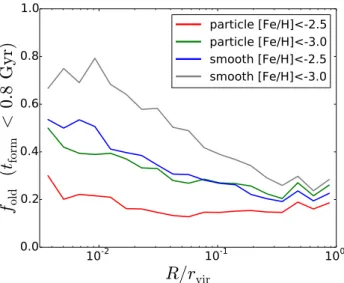
Figure 8. The fraction of most metal-poor stars that are old as a function of radius. Shown here is the median value for all L2 galaxies (corresponding to the blue thick line in the bottom panel of Fig.2; the blue line in this figure is identical to that) for two different metallicity calculations: an SPH-smoothed metallicity (our fiducial choice) and a particle metallicity (no metal mixing at all). We additionally show two different cutoff values for the most metal-poor stars: [Fe/H]<−2.5 (as used throughout the paper) and [Fe/H]<−3.0.
and is hence ignored in all other work mentioned here, including our own (but see for a very similar approach, Ishiyama et al.2016). Gao et al. (2010) find the minihaloes to be strongly clustered in space, therefore limiting the number of final building blocks that contain them as most of them merge in time. At the present day, the environments where the first stars are found are again centrally concentrated, but they also report that a significant fraction (over 20 per cent, we find a very similar percentage; see also Section 4) remains in the satellites that are presently surrounding the Milky Way. In Gao et al. (2010), none of the baryonic processes are mod-elled after the first generation of stars, so the present-day properties of these satellites can only be compared on the basis of their dark matter properties, which, however, do seem to be comparable to the surviving satellites that we observe around the Milky Way today.
6.2.1 The role of metal mixing
The many differences between the models once more illustrate how the results at early epochs and low metallicities are sensitive to the assumptions that are made and the modelling prescriptions that are used. Here, we investigate in more detail in particular the sensitivity of our results to the assumptions on metal mixing. As described in Section 3.1, our fiducial model includes an SPH kernel-smoothed mixing prescription. However, in the APOSTLE simulations we also store the individual star particle metallicities, inherited from unmixed gas. In general, we find that all qualitative results are robust to either calculation of the metallicity and that most quantitative re-sults show only very minor variations (for instance, the percentages of the different populations that are located outside an 8 kpc radius as labelled in Figs3and7are robust to the metallicity prescription used).
However, there are significant changes in the radial dependence of the fraction of the most metal-poor stars that are old. This is illustrated in Fig.8, where the median fraction for all L2 galaxies is shown as a function of radius for both types of metallicity estimates
(the blue line corresponds to the blue thick line in the bottom panel of Fig.2). Fig.8additionally shows that there is a degeneracy be-tween the amount of mixing and the cutoff [Fe/H] used to determine whether a star is metal poor. For the particle metallicity scheme, we still see a clear gradient when we adopt a lower metallicity thresh-old. Whereas SPH-based results will generally underpredict mixing and use particle metallicities, semi-analytic models often assume perfect mixing of all gas within a system. Our implementation of smoothed metallicities lies in between these two extremes, but while it decreases the severity of the sampling aspect of the mixing prob-lem within SPH, it does not solve it either (Wiersma et al.2009b). Clearly, quantitative results from any prescription quoting the frac-tion of metal-poor stars that are old in a certain Galactic region should be treated with caution. They are very dependent on the assumptions for metal mixing, a process that is uncertain.
C O N C L U S I O N S
We have investigated the properties of the most metal-poor and old-est stellar populations in the APOSTLE simulations of Local Group analogues, focusing, in particular, on their present-day distribution. As illustrated in Fig.2, we find that the highest fraction of either of these populations can be found at larger radii, making the outer halo an obvious hunting ground for these stellar populations. When looking at stars that are both metal poor and old, we again find that the majority of them (≈60 per cent) can currently be found at radii greater than that of the solar neighbourhood (>8 kpc, see Fig.3). However, if one could observationally disentangle all metal-poor stars in the Milky Way from their more metal-rich peers, the simu-lations suggest that those at the centre are the most likely to be old and even to have formed before the epoch of reionization. Quali-tatively, this result strengthens the conclusions of previous papers in this area that were based on a semi-analytic framework. Quanti-tatively though, many differences can be found that can be ascribed to the various prescriptions that are used. Most notably, we show in Fig.8that quantitative results are sensitive to the metal mixing prescription.
The coming decade promises to be fruitful for the further study of the extremely metal poor and old Galaxy, with various surveys underway to mine these stars in various environments. One of the aims of this work is to provide guidance for any survey efforts designed to look for the most metal-poor stars. We find that surveys of the outer halo are likely to uncover the sites of very early star formation in various environments. Roughly half of the stars formed before the epoch of reionization can be found at radii>8 kpc today, as well as on average≈75 per cent of the pristine stars (see Fig.7). Whether these sites are truly free of the impact of the first stars forming elsewhere, either in the form of pollution with metals, or radiation or kinematic feedback, remains an open question that such surveys could help to constrain.
distinguished by their large fraction of old populations (>10 Gyr) and alowfraction of metal-poor stars.
AC K N OW L E D G E M E N T S
We would like to thank Ryan Leaman, Nicolas Martin and Chris Brook for insightful discussions on this work, as well as the anony-mous referee for thoughtful comments that helped to improve this manuscript. ES and KAO are grateful to the Mainz Institute for Theoretical Physics (MITP) for its hospitality and its partial sup-port during the completion of this work. KAO is grateful for the generous hospitality of the Leibniz Institute for Astronomy Pots-dam (AIP). ES gratefully acknowledges funding by the Emmy Noether programme from the Deutsche Forschungsgemeinschaft (DFG). This work was supported by the Science and Technology Facilities Council (grant number ST/F001166/1). CSF acknowl-edges ERC Advanced Grant 267291 ‘COSMIWAY’. This work used the DiRAC Data Centric system at Durham University, op-erated by the Institute for Computational Cosmology on behalf of the STFC DiRAC HPC Facility (www.dirac.ac.uk). This equip-ment was funded by BIS National E-infrastructure capital grant ST/K00042X/1, STFC capital grant ST/H008519/1, STFC DiRAC Operations grant ST/K003267/1 and Durham University. DiRAC is part of the National E-Infrastructure. This research has made use of NASA’s Astrophysics Data System. The research was supported in part by the European Research Council under the European Union’s Seventh Framework Programme (FP7/2007-2013)/ERC Grant agreement 278594-GasAroundGalaxies. TS acknowledges the support of the Academy of Finland grant 1274931.
R E F E R E N C E S
Abel T., Bryan G. L., Norman M. L., 2002, Science, 295, 93 Allende Prieto C. et al., 2014, A&A, 568, A7
Asplund M., Grevesse N., Sauval A. J., Scott P., 2009, ARA&A, 47, 481 Beers T. C., Preston G. W., Shectman S. A., 1985, AJ, 90, 2089 Beers T. C. et al., 2012, ApJ, 746, 34
Bland-Hawthorn J., Gerhard O., 2016, ARA&A, 54, 529 Bonifacio P. et al., 2015, A&A, 579, A28
Bovill M. S., Ricotti M., 2009, ApJ, 693, 1859 Bovill M. S., Ricotti M., 2011a, ApJ, 741, 17 Bovill M. S., Ricotti M., 2011b, ApJ, 741, 18 Bromm V., 2013, Rep. Prog. Phys., 76, 112901
Brook C. B., Kawata D., Scannapieco E., Martel H., Gibson B. K., 2007, ApJ, 661, 10
Brown T. M. et al., 2014, ApJ, 796, 91 Caffau E. et al., 2011, Nature, 477, 67
Campbell D. J. R. et al., 2016, preprint (arXiv:1603.04443) Carollo D. et al., 2007, Nature, 450, 1020
Carollo D. et al., 2010, ApJ, 712, 692
Carollo D., Freeman K., Beers T., Placco V., Tumlinson J., Martell S., 2014, ApJ, 788, 180
Casey A. R., Schlaufman K. C., 2015, ApJ, 809, 110 Chabrier G., 2003, PASP, 115, 763
Christlieb N., 2003, in Schielicke R. E. ed., Rev. Mod. Astron., Vol. 16, The Cosmic Circuit of Matter. Wiley, New York, p. 191
Christlieb N., Wisotzki L., Graßhoff G., 2002, A&A, 391, 397 Cooper A. P. et al., 2010, MNRAS, 406, 744
Cooper A. P., Parry O. H., Lowing B., Cole S., Frenk C., 2015, MNRAS, 454, 3185
Crain R. A. et al., 2015, MNRAS, 450, 1937 Dalla Vecchia C., Schaye J., 2012, MNRAS, 426, 140
de Jong J. T. A., Yanny B., Rix H.-W., Dolphin A. E., Martin N. F., Beers T. C., 2010, ApJ, 714, 663
Durrell P. R., Harris W. E., Pritchet C. J., 2004, AJ, 128, 260
Fattahi A. et al., 2016, MNRAS, 457, 844 Frebel A., Bromm V., 2012, ApJ, 759, 115 Frebel A. et al., 2005, Nature, 434, 871 Frebel A. et al., 2006, ApJ, 652, 1585
Frebel A., Kirby E. N., Simon J. D., 2010, Nature, 464, 72 Frebel A., Simon J. D., Kirby E. N., 2014, ApJ, 786, 74
Frebel A., Chiti A., Ji A. P., Jacobson H. R., Placco V. M., 2015, ApJ, 810, L27
Gao L., Theuns T., Frenk C. S., Jenkins A., Helly J. C., Navarro J., Springel V., White S. D. M., 2010, MNRAS, 403, 1283
Gilbert K. M. et al., 2014, ApJ, 796, 76
Gilmore G., Norris J. E., Monaco L., Yong D., Wyse R. F. G., Geisler D., 2013, ApJ, 763, 61
Greif T. H., 2015, Comput. Astrophys. Cosmol., 2, 3 Haardt F., Madau P., 2012, ApJ, 746, 125
Hansen T. et al., 2014, ApJ, 787, 162
Hartwig T., Bromm V., Klessen R. S., Glover S. C. O., 2015, MNRAS, 447, 3892
Helmi A., 2008, A&AR, 15, 145
Hobbs A., Read J., Power C., Cole D., 2013, MNRAS, 434, 1849 Howes L. M. et al., 2015, Nature, 527, 484
Howes L. M. et al., 2016, MNRAS, 460, 884
Ishiyama T., Sudo K., Yokoi S., Hasegawa K., Tominaga N., Susa H., 2016, ApJ, 826, 9
Jablonka P. et al., 2015, A&A, 583, A67 Jenkins A., 2013, MNRAS, 434, 2094
Ji A. P., Frebel A., Chiti A., Simon J. D., 2016, Nature, 531, 610
Karlsson T., Bromm V., Bland-Hawthorn J., 2013, Rev. Mod. Phys., 85, 809 Kaufmann T., Mayer L., Wadsley J., Stadel J., Moore B., 2006, MNRAS,
370, 1612
Keller S. C. et al., 2007, PASA, 24, 1 Keller S. C. et al., 2014, Nature, 506, 463
Kereˇs D., Vogelsberger M., Sijacki D., Springel V., Hernquist L., 2012, MNRAS, 425, 2027
Kirby E. N., Simon J. D., Geha M., Guhathakurta P., Frebel A., 2008, ApJ, 685, L43
Kirby E. N. et al., 2010, ApJS, 191, 352 Komatsu E. et al., 2011, ApJS, 192, 18
Komiya Y., Habe A., Suda T., Fujimoto M. Y., 2010, ApJ, 717, 542 McConnachie A. W., 2012, AJ, 144, 4
McKee C. F., Tan J. C., 2008, ApJ, 681, 771 Marigo P., 2001, A&A, 370, 194
Muratov A. L., Gnedin O. Y., Gnedin N. Y., Zemp M., 2013a, ApJ, 772, 106 Muratov A. L., Gnedin O. Y., Gnedin N. Y., Zemp M., 2013b, ApJ, 773, 19 Norris J. E., Christlieb N., Korn A. J., Eriksson K., Bessell M. S., Beers
T. C., Wisotzki L., Reimers D., 2007, ApJ, 670, 774 Norris J. E. et al., 2013, ApJ, 762, 28
Parry O. H., Eke V. R., Frenk C. S., Okamoto T., 2012, MNRAS, 419, 3304
Pawlik A. H., Schaye J., 2008, MNRAS, 389, 651 Portinari L., Chiosi C., Bressan A., 1998, A&A, 334, 505 Romano D., Starkenburg E., 2013, MNRAS, 434, 471 Salvadori S., Ferrara A., 2009, MNRAS, 395, L6
Salvadori S., Schneider R., Ferrara A., 2007, MNRAS, 381, 647
Salvadori S., Ferrara A., Schneider R., Scannapieco E., Kawata D., 2010, MNRAS, 401, L5
Salvadori S., Tolstoy E., Ferrara A., Zaroubi S., 2014, MNRAS, 437, L26 Salvadori S., Sk´ulad´ottir ´A., Tolstoy E., 2015, MNRAS, 454, 1320 Sawala T. et al., 2016, MNRAS, 457, 1931
Scannapieco E., Schneider R., Ferrara A., 2003, ApJ, 589, 35
Scannapieco E., Kawata D., Brook C. B., Schneider R., Ferrara A., Gibson B. K., 2006, ApJ, 653, 285
Schaller M., Dalla Vecchia C., Schaye J., Bower R. G., Theuns T., Crain R. A., Furlong M., McCarthy I. G., 2015, MNRAS, 454, 2277 Schaye J., 2004, ApJ, 609, 667
Schaye J., Dalla Vecchia C., 2008, MNRAS, 383, 1210 Schaye J. et al., 2015, MNRAS, 446, 521
Sk´ulad´ottir ´A., Tolstoy E., Salvadori S., Hill V., Pettini M., Shetrone M. D., Starkenburg E., 2015, A&A, 574, A129
Smith B. D., Wise J. H., O’Shea B. W., Norman M. L., Khochfar S., 2015, MNRAS, 452, 2822
Springel V. et al., 2008, MNRAS, 391, 1685 Starkenburg E. et al., 2010, A&A, 513, A34 Starkenburg E. et al., 2013, A&A, 549, A88
Starkenburg E., Shetrone M. D., McConnachie A. W., Venn K. A., 2014, MNRAS, 441, 1217
Tafelmeyer M. et al., 2010, A&A, 524, A58
Thielemann F.-K. et al., 2003, in Hillebrandt W., Leibundgut B., eds, From Twilight to Highlight: The Physics of Supernovae. Springer-Verlag, Berlin, p. 331
Tornatore L., Ferrara A., Schneider R., 2007, MNRAS, 382, 945 Trenti M., Stiavelli M., Michael Shull J., 2009, ApJ, 700, 1672 Tumlinson J., 2010, ApJ, 708, 1398
Venn K. A. et al., 2012, ApJ, 751, 102
Weisz D. R., Dolphin A. E., Skillman E. D., Holtzman J., Gilbert K. M., Dalcanton J. J., Williams B. F., 2014, ApJ, 789, 148
White S. D. M., Springel V., 2000, in Weiss A., Abel T. G., Hill V., eds, The First Stars. Springer-Verlag, Berlin, p. 327
Wiersma R. P. C., Schaye J., Smith B. D., 2009a, MNRAS, 393, 99 Wiersma R. P. C., Schaye J., Theuns T., Dalla Vecchia C., Tornatore L.,
2009b, MNRAS, 399, 574
Wise J. H., Turk M. J., Norman M. L., Abel T., 2012, ApJ, 745, 50 Xu H., Norman M. L., O’Shea B. W., Wise J. H., 2016, ApJ, 823, 140 Yong D. et al., 2013, ApJ, 762, 26
Yoshida N., Bromm V., Hernquist L., 2004, ApJ, 605, 579
A P P E N D I X A : T H E E F F E C T O F R E S O L U T I O N
Star formation processes and the general build-up of mass in galax-ies may depend on the simulation resolution. Three different resolu-tion versions have been run for the APOSTLE simularesolu-tions, allowing us to investigate the robustness of our results to variations in the particle mass.
Fig.A1shows the fraction of oldest or most metal-poor popula-tions (according to the definipopula-tions given in Section 3) as a function of stellar mass for galaxies within 2 Mpc of the main MW/M31 pair in each simulation. Different colours are used for different resolution runs. From this figure, it becomes clear that for the lowest resolution simulations, resolution indeed plays a role. The galaxies generally have a higher fraction of oldest or, respectively, most metal-poor stars than equal mass galaxies in higher resolution runs. On the other hand, the intermediate and highest resolution simulations form a continuous sequence with large overlap. Additional analysis of the fraction of stars that are both metal poor and old – a quantity that is
Figure A1. The fraction of old (formation time<0.8 Gyr after the big bang; top panel) or most metal-poor ([Fe/H]<−2.5; bottom panel) populations as a function of stellar mass for galaxies within 2 Mpc of the main MW+M31 pair in each simulation. Filled symbols indicate galaxies within 300 kpc from either one of the main host galaxies. Black, blue and red points represent galaxies with the low (L3), intermediate (L2) and high resolution (L1) simulations, respectively.
central to our analysis in Section 4 – reveals that for all overlapping galaxy stellar mass bins, the distribution of the fractions of oldest and most metal-poor stars is consistent between the high and inter-mediate resolution simulations. A Kolmogorov-Smirnov (KS) test shows that the probability of the high- and intermediate-resolution distributions being drawn from a similar parent population is always larger than 0.18 for all mass bins.
![Figure 6. The fraction of age >10 Gyr populations in dwarf galaxies and the fraction of stars with [Fe /H] < −2.5, colour coded by the fraction of these most metal-poor stars that are old (formed before 0.8 Gyr after the big bang)](https://thumb-us.123doks.com/thumbv2/123dok_us/8278199.2192298/8.892.71.425.79.441/figure-fraction-populations-galaxies-fraction-colour-fraction-formed.webp)
![Figure 7. Four different views on the six high-resolution main galaxies. Shown are the pristine population, completely devoid of metals (top left), [Fe /H] <](https://thumb-us.123doks.com/thumbv2/123dok_us/8278199.2192298/9.892.86.802.77.976/figure-different-resolution-galaxies-shown-pristine-population-completely.webp)