Three essays on intellectual property rights in developing countries

Three Essays on Intellectual Property Rights

in Developing Countries

by

Kristie N. Briggs

A dissertation submitted to the faculty of the University of North Carolina at Chapel Hill in partial fulfillment of the requirements for the degree of Doctor of Philosophy in the Department of Economics.

Chapel Hill 2008

Approved by:

Alfred J. Field, Jr., Advisor

Scott A. Baker, Reader

Patrick J. Conway, Reader

Neville R. Francis, Reader

c

2008

ABSTRACT

KRISTIE N. BRIGGS: Three Essays on Intellectual Property Rights in Developing Countries

(Under the direction of Alfred J. Field, Jr.)

Developing countries today face different international policies and pressures than did

the currently industrialized countries when they were in the midst of the development

pro-cess. Recent external pressures on developing countries to implement intellectual property

rights (IPRs) are just one example. In practice many developing countries have chosen to

implement strong patent policies, despite the fact that these countries have limited capacity

for innovation. Developing countries are instead better characterized as “imitators” that

learn from technology transferred from innovating (industrialized) countries. Therefore,

im-plementing IPRs would seem counterintuitive for developing countries as it restricts their

ability to imitate. Despite the possible costs, many international organizations argue that

developing countries do, in fact, benefit from implementing IPRs via increased trade and

foreign direct investment. However, the true impact of IPR policy in developing countries

remains largely unclear. This dissertation untangles some of the links between IPRs, trade,

and development by focusing on a particular aspect of this issue in each of three essays. The first essay considers how a country’s choice in IPRs relates to their stage in

devel-opment. The essay is novel in that it brings to light evidence that a country’s choice in

IPRs as it develops (the longitudinal relationship) has a distinctly different IPR-per capita

GDP relationship than it has when considering the IPR choice for a variety of countries in

different stages of development, but at one point in time (the cross-sectional relationship).

The second essay looks at whether IPRs in developing countries stimulate high technology

exports from industrialized countries. By analyzing an array of different high technology

ex-ports to developing countries, it was determined which types of high technology goods were

strengthened domestic IPRs. The third essay explores whether stronger IPRs in developing

countries will stimulate their export activity. The acquisition of IPRs in developing countries

is found to have a significantly positive impact on developing country exports, suggesting a

ACKNOWLEDGEMENTS

I would like to express my appreciation for my advisor, Alfred Field, Jr. He has provided me with time, guidance, and encouragement throughout the course of my research. I also

wish to thank my committee members: Scott Baker, Patrick Conway, Neville Francis, and

David Guilkey for their insight and advice. I thank Walter Park for providing data. I also

thank my fellow graduate students, especially Charlie, Tia, and Mike for helping me along

the way. I would like to thank my sister, Jennifer, for her unending support, and both Jen

and Art for never making me pay for a single meal throughout all of graduate school!

Lastly, I would like to thank my parents for all the encouragement and sacrifices they

made that helped me reach where I am today. They have truly shown me value of hard

TABLE OF CONTENTS

LIST OF TABLES . . . x

LIST OF FIGURES . . . xii

1 Introduction . . . 1

2 Intellectual Property Rights and Development: A Longitudinal vs. Cross Sectional Study . . . 4

2.1 Introduction . . . 4

2.2 Review of Literature . . . 5

2.3 Theoretical Model . . . 8

2.3.1 Chen and Puttitanun’s Model . . . 8

2.3.2 A Revised Longitudinal Theory . . . 14

2.4 Linking Theory and Empirical Analysis . . . 19

2.4.1 The Ginarte-Park IPR Index . . . 19

2.5 Exploring the Longitudinal Data . . . 21

2.5.1 Pooled Data Analysis of the IPR-per capita GDP relationship . . . 25

2.6 The Fully Specified Model . . . 27

2.6.1 Estimating IPRs . . . 29

2.6.2 Endogeneity of IPRs and per capita GDP . . . 32

2.6.3 Estimating per capita GDP . . . 32

2.6.4 Specification of the System of Equations . . . 34

2.6.5 Empirical Results . . . 36

2.7 A Cross-Sectional Explanation for the U-shape . . . 38

2.7.1 The Role of International Pressure in IPR Choice . . . 39

2.8 Conclusion . . . 53

3.1 Introduction . . . 56

3.2 Review of Literature . . . 58

3.2.1 Literature on IPRs and Trade in the North-South Context . . . 58

3.2.2 Empirical Research on IPRs and Bilateral Trade Flows . . . 59

3.2.3 Review of Literature on Gravity Models . . . 61

3.3 Theoretical Model . . . 62

3.3.1 The Story . . . 62

3.3.2 The Model . . . 63

3.3.3 What Impacts the Optimal Quantity to Produce and Export? . . . 70

3.3.4 Predictions about the Empirical Results . . . 71

3.4 Empirical Estimation . . . 73

3.4.1 The Gravity Model . . . 74

3.4.2 Country and High Technology Good Specifications . . . 79

3.4.3 Results . . . 80

3.5 Conclusion . . . 85

4 Do Intellectual Property Rights Increase Export Activity in Developing Countries? . . . 94

4.1 Introduction . . . 94

4.2 Relevant Literature . . . 95

4.3 Theoretical Model . . . 97

4.3.1 Exports of Newly Innovated Goods . . . 97

4.3.2 Exports of Existing Goods . . . 99

4.3.3 Total Export Activity . . . 103

4.4 Empirical Estimation . . . .104

4.4.1 Estimating Equation for Exports . . . 104

4.4.2 Problems with Endogeneity . . . 106

4.4.3 Data Description . . . 110

4.4.4 Empirical Results . . . 113

A Appendix for Essay One . . . 121

A.1 Summary of Empirical Results from Past Literature . . . 121

A.2 Ginarte-Park Index of Patent Rights . . . 123

A.3 Identifying the “Critical” Cross-Sectional Year . . . 124

A.4 Stage One Results for the Fully Specified Model . . . 127

A.5 Cross-Sectional Results Accounting for Regional Effects . . . 128

B Appendix for Essay Two . . . 129

B.1 Explanations Proposed by Primo Braga and Fink . . . 129

B.2 Determining “Value Added” Categories . . . 130

B.3 Analysis of Low & Lower-Middle Income Countries . . . 131

C Appendix for Essay Three . . . 142

C.1 USPTO Patent Count Data . . . 142

C.2 First Stage Results for Essay 3 . . . 144

LIST OF TABLES

2.1 Group Classification used in Pooled Regression Analysis . . . 26

2.2 Pooled Regression Using Panel Data . . . 28

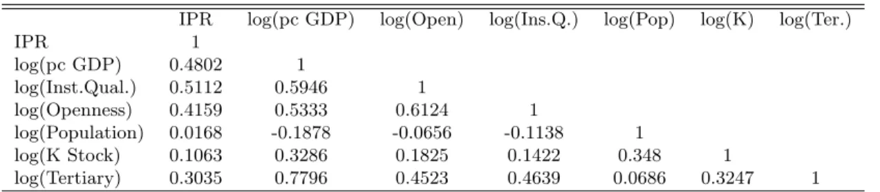
2.3 Descriptive Statistics . . . 36

2.4 Correlation Matrix . . . 36

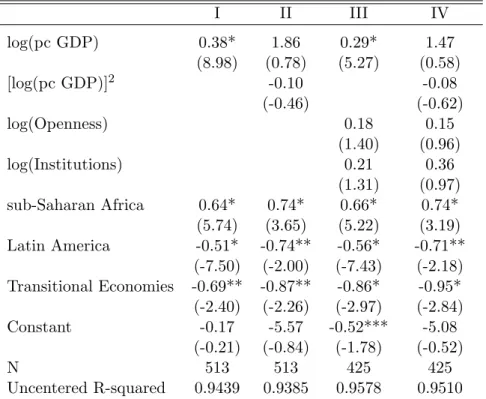
2.5 Choice of IPRs: The Fully Specified Model . . . 37

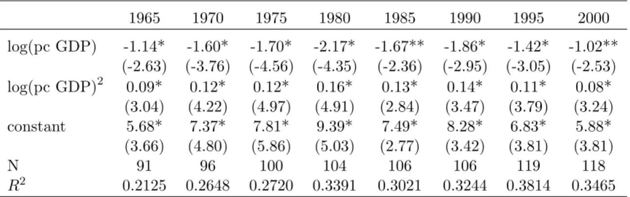
2.6 Cross Section of IPRs for Each Available Year . . . 38

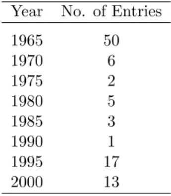
2.7 Composition of the Critical Cross-Section of Years . . . 45

2.8 Critical Cross Sectional IPR Decision . . . 48

2.9 Composition of Critical Cross-Section: Omitting 1885-1960 . . . 52

2.10 Critical Cross Sectional IPR Decision: Omitting 1885-1960 . . . 54

3.1 Composition of Aggregate High Technology Goods . . . 81

3.2 Value Added Categories . . . 82

3.3 Developed Country High Tech Exports to Low Income Countries . . . 86

4.1 Descriptive Statistics: Low & Lower-Middle Income Countries . . . 113

4.2 Bilateral Exports with Inward FDI in Current Period . . . 115

4.3 Bilateral Exports with Lagged Inward FDI . . . 116

4.4 Descriptive Statistics: High Income Countries Only . . . 118

4.5 Bilateral Exports (High Income Countries) . . . 119

A.1 IPR Regression Results from Past Literature . . . 121

A.2 Preliminary Results for IPR Choice . . . 122

A.3 Ginarte-Park Index of Patent Rights: Categories and Calculations . . . 123

A.4 Specification for the ‘Critical” Cross-Sectional Year . . . 124

A.5 Stage One Results: log(Per Capita GDP) . . . 127

B.1 Developed Country Exports to Low & Lower-Middle Income Countries . . . . 134

LIST OF FIGURES

2.1 Legal vs. Effective IPRs . . . 15

2.2 Selected Country Specific IPR Graphs . . . 24

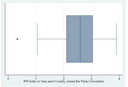
2.3 Box Plot of IPRs showing Indonesia as an Outlier . . . 49

2.4 Scatter Plot of Critical Cross-Section when Indonesia is Included . . . 50

2.5 Scatter Plot of Critical Cross-Section when Indonesia is Omitted . . . 50

Chapter 1

Introduction

Developing countries today face different international policies and pressures than did

the currently industrialized countries when they were in the midst of the development

pro-cess. Recent external pressures on developing countries to implement intellectual property

rights (IPRs) are just one example. In practice many developing countries have chosen to

implement strong patent policies, despite the fact that these countries have limited capacity

for innovation. Developing countries are instead better characterized as “imitators” that

learn from technology transferred from innovating (industrialized) countries. Therefore,

im-plementing IPRs would seem counterintuitive for developing countries as it restricts their

ability to imitate. Despite the possible costs, many international organizations argue that

developing countries do, in fact, benefit from implementing IPRs via increased trade and

foreign direct investment. However, the true impact of IPR policy in developing countries remains largely unclear. This dissertation untangles some of the links between IPRs, trade,

and development by focusing on a particular aspect of this issue in each of three essays.

The first essay examines the role that a country’s stage of development plays in its choice

of IPRs. The essay is novel in that it brings to light evidence that a country’s choice in IPRs

as it develops (the longitudinal relationship) has a distinctly different IPR-per capita GDP

relationship than it has when considering the IPR choice for a variety of countries in different

stages of development, but at one point in time (the cross-sectional relationship). Past

empirical observations on a panel of countries over time have found a U-shape relationship

countries. A longitudinal U-shape, however, does not correspond to historical observation;

countries generally maintain or increase IPRs over time and demonstrate a similar trend as

they progress through stages of development. This paper argues that the well known U-shape

relationship between IPRs and per capita GDP is instead a result of cross country differences

originating in the year that each country first chooses to implement IPRs. Distinguishing

between the longitudinal and cross-sectional relationship between IPRs and per capita GDP

will enable researchers to accurately estimate and interpret the effects of IPRs when using

panel data.

The second essay examines how developed-country exports of high technology goods to developing countries are stimulated by IPRs in developing countries. One argument for

im-plementing strong IPRs in developing countries is that they attract greater high technology

exports from industrialized countries, which should consequently lead to economic growth.

Past empirical observation using an aggregate of high technology goods, however, has

sug-gested that bilateral exports of high technology goods is not impacted by the level of IPRs in

the importing country. A disaggregated analysis of high technology goods provides a more

precise insight into which high technology goods developed countries export in the presence

of stronger developing country IPRs. The impact of developing country IPRs on high

tech-nology exports from developed countries is contingent on a combination of variables such as

production and adaptation costs and whether innovations in the high technology group can

readily be used in domestic production processes. Innovations in high technology groups

such as potassic fertilizers, synthetic yarn, and artificial fibers are arguably very pertinent

to production in developing countries that specialize in agricultural and textile production.

Therefore, the markup in price for these high technology innovations is relatively high. In addition, marginal production and adaptation costs of innovated goods in these categories

are expectedly low. The combination of high markups and low marginal costs result in

a dominant market power effect when developing countries increase IPRs, indicating that

an increase in IPRs does not increase developed country exports of these goods. On the

other hand, industrialized high technology exports that have relatively higher production

mar-ket expansion effect. In this latter case, stronger IPRs in developing countries lead to an

increased receipt of high technology goods from industrialized countries.

The third essay examines the impact that patent policies have on export activity in

developing countries. Outward looking development policies centered on export promotion

have become increasingly popular strategies for stimulating economic growth in developing

countries. At the same time, many developing countries have adopted IPRs in recent years,

often upon the suggestion of industrialized countries and international organizations. This

paper explores the possible link between export promotion and IPR policies by examining

Chapter 2

Intellectual Property Rights and

Development: A Longitudinal vs. Cross

Sectional Study

2.1

Introduction

This paper examines the role that a country’s stage of development plays in its choice

of intellectual property rights (IPRs). Past empirical observations on a panel of countries

over time have found a U-shape relationship between IPRs and per capita GDP and taken it to imply a longitudinal U-relationship within countries. A longitudinal U-shape, however,

is counterfactual. Countries generally maintain or increase IPRs over time and, therefore,

expectedly demonstrate a similar trend as they progress through stages of development.

This paper argues that the well known U-shape is a result of cross country differences

originating in the year that each country first chooses to implement IPRs, rather than a

result of a longitudinal trend. To summarize, the conjecture of this paper is two-fold. First,

the longitudinal relationship between IPRs and per capita GDP is monotonically increasing

(rather than U-shaped). Second, a U-shape relationship between IPRs and per capita GDP

exists cross-sectionally, when a variety of countries in different stages of development are

examined at one point in time.

IPRs initially decrease and later increase as per capita GDP increases in a given country.

The downward portion of a longitudinal U relationship is generally not obtained as countries

generally do not actively weaken IPRs, barring a regime change or other alteration in their

political economy. The longitudinal U conclusion was largely drawn from the results of panel

data. Although longitudinal extrapolations of panel data are common, they are not always

valid. The significant non-monotonic link empirically discovered using panel data is a result

of cross sectional influences, not longitudinal influences. Interpretation of a cross-sectional

U-shape relationship between IPRs and per capita GDP would mean that, in a given year,

least developed countries exhibit stronger IPRs than middle-income developing countries, while high-income countries again exhibit strong IPRs.

The cross-sectional U-shape between IPRs and per capita GDP can be attributed to

cross country differences in IPRs in the year IPRs were first implemented. In the year that

countries first implemented IPRs, the least developed countries implement stronger patent

rights, partially because these countries are the most vulnerable to international pressures to

do so. Middle-income developing countries exercise more autonomy, however, and implement

weaker patent rights that enable them to greater utilize imitation as a pathway for growth.

Finally, when high-income countries first implement IPRs they implement relatively strong

IPRs as they have innovation related incentives to do so.

This paper contributes to the IPR literature by making a distinction between the

longi-tudinal and cross-sectional relationship between IPRs and per capita GDP, and by

demon-strating that the U-shape relationship observed in panel data is a result of cross sectional

differences in countries at different stages of development. Establishing this will enable

researchers to accurately estimate and interpret the effects of IPRs when using panel data.

2.2

Review of Literature

Three key contributions to the literature on the U-shape relationship between IPRs

Braga, Fink, and Sepulveda (2000).1 In addition, Ginarte and Park (1997) made ancillary contributions.

Ginarte and Park introduced their IPR index in 1997. In the same article, they

ex-amined the characteristics that influenced a country’s choice in IPRs. Ginarte and Park

concluded that a country’s level of per capita income, research and development (R&D),

political freedom, openness to trade, and secondary school enrollment rates together

deter-mine a country’s choice in IPRs. While Ginarte and Park concluded a country’s stage in

development significantly impacts its choice of IPRs, they did not consider the possibility

of a U-shape relationship.2 Efforts to pinpoint the exact relationship between these two variables has since emerged.

Maskus (2000) empirically observed a U-shape link between per capita income and IPRs.

He came to this conclusion in two separate analysis. He found this U-shape link in an

expansion of his work with Penubarti (1995) using a 1984 cross-section of countries and

the Rapp and Rozek IPR Index, as well as in analysis using the Ginarte and Park IPR

Index for a panel of countries in 1985 and 1990. The U-shape link remained significant

even when Maskus expanded the IPR regression equation to include independent variables

such as R&D expenditures as a proportion of GDP, secondary school enrollment, political

freedom, openness to trade, and market freedom. (These results can be found in Appendix

A.1.) While Maskus empirically observed the U-shape, and interpreted it longitudinally to

explain a country’s choice in IPRs as it develops, he did not provide a theoretical explanation

for the U-shape.

Chen and Puttitanun (2005) provided the first theoretical explanation for the U-shape

relationship between IPRs and per capita GDP by using a game theoretic approach to model a country’s choice of optimal IPRs. (This model will be outlined in detail in the

next section.) They then tested their theory using a panel of 62 developing countries for

the years 1985, 1990, 1995, and 2000. Chen and Puttitanun concluded that countries in 1

Most analysis of the U-shape has been explored using panel data for many countries over a series of years, while some has been strictly cross sectional analysis.

2_{The data used by Ginarte and Park include a panel of 48 developed and developing countries for the}

the earliest stages of development implement higher IPRs to attract foreign technologies so

that they can imitate and grow. As a country gains access to foreign technologies, however,

stronger IPRs actually hinder its ability to imitate. As a result, Chen and Puttitanun argue

that these countries decrease the strength of IPRs so they can utilize imitation to foster

technological advancement. Once a certain level of development is reached,3 countries are capable of obtaining benefits from domestic innovation and therefore begin to strengthen

their IPRs.4 Chen and Puttitanun’s theoretical argument for the U-shape is examined thoroughly in the next section, as this paper suggests a revised longitudinal model for the

IPR-per capita GDP relationship.

In Chen and Puttitanun’s empirical estimation, they incorporate a two-stage regression

in their evaluation of the U relationship where they estimate IPRs in the first stage and then

estimate innovation as a function of IPRs in the second stage.5 (This paper alternatively argues that per capita GDP directly influences IPRs.) Chen and Puttitanun ultimately

found that there is a significant U-shape link between IPRs and per capita GDP.

Primo Braga, Fink, and Sepulveda (2000) consider the relationship between IPRs and

per capita GDP for a cross section of countries in the year 1975. Although the U-shape is

not a primary focus, the Primo Braga, Fink, and Sepulveda paper is important for a couple

of reasons. First, it finds a statistically significant relationship between IPRs and per capita

GDP using a strictly cross-sectional analysis for the year 1975. This is an important result

as it provides preliminary evidence that the U-shape configuration captured by panel data

could actually be driven by the cross-sectional variation. Secondly, in discussion unrelated

to the U-shape, Primo Braga, Fink, and Sepulveda claim that one determinant of IPRs

in developing countries is the international pressures they feel from more industrialized 3_{Chen and Puttitanun use development and technological advancement interchangeably in their model.}

4

Chen and Puttitanun argue that even developing countries benefit from domestic innovation, pointing out that the number of domestic patent application in 1985-1995 were particularly high in Brazil, India, South Africa, and South Korea.

5

countries. In a similar line of thinking, this paper postulates that developing countries’

vulnerability to international pressures are directly related to the cross-sectional U-shape

between IPRs and per capita GDP.

Empirical results for papers discussed in this literature review found in AppendixA.1.

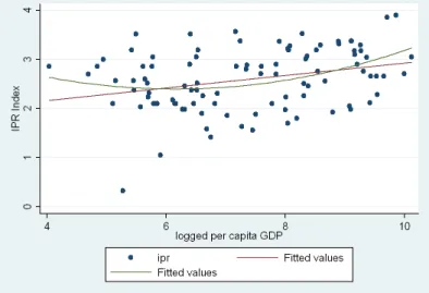
Primo Braga, Fink, and Sepulveda did not provide specific results, but rather a scatter plot

and the associated best-fit monotonic line.

2.3

Theoretical Model

The theoretical model explaining the U-shape link between IPRs and per capita GDP

found in Chen and Puttitanun (2005) is the only theory I could locate addressing the

possible relationship to date. In their model Chen and Puttitanun (CP) find support for

a longitudinal U-shape link between IPRs and per capita GDP. Their model, however,

considers a country’s IPRs written into law and does not explicitly address how enforcement

of these laws may impact perceived IPRs. The Ginarte-Park IPR index, which is most often

used in empirical analysis of IPRs, includes a measure for enforcement. The suggested

revised model for the longitudinal relationship between IPRs and per capita GDP explicitly

considers enforcement of IPRs.

2.3.1 Chen and Puttitanun’s Model

The CP theoretical model takes a game theoretic approach to finding how economic

growth affects optimal IPRs. In their model, the developing (domestic) country chooses its

level of IPR protection, β ∈[0; 1], where β= 0 indicates no protection and β = 1 indicates perfect protection. In addition, the parameter θ∈(0; 1] is a measure of the country’s level of development such that higher levels of θindicate greater development.

The domestic economy has two sectors, A and B. Sector A is comprised of two firms, a

foreign (developed country) firm, F, and a domestic (developing country) firm, D. Sector B

is comprised of two domestic firms, L and M. Each sector produces a different good and has

one imitating firm. Firms F and L are innovators in Sectors A and B, respectively, while

firms D and M are imitators, respectively. Sectors A and B are linked through the shared

IPRs.

In Sector A, the foreign firm sells a product of exogenous quality µF, which is under

a patented technology. Domestic firm D may produce the good in Sector A, but with a

quality level µD(β, θ) = µ0 +µFφ(θ)[1−α(β)] such that µD < µF by assumption. The

quality of the domestically produced good is dependent on the exogenous quality of the

foreign produced good, as well as firm D’s imitative abilities, represented by the parameter

φ(θ), and the limitation to imitation that results from stronger IPRs, α(β). In addition, for everyθ, 0≤φ(θ)≤1,φ0(θ)>0,α0(β)>0, α(1) = 1, and 0≤µ0 ≤µF(1−φ(1)). Countries

that are more developed (as identified by higher levels of θ) have greater imitative ability.

Perfect IPR protection (as identified by β = 1) results in no imitative capabilities for firm

D. Finally, all firms in Sector A have a constant unit cost ofcA∈[0, µ0].

In Sector B, firm L produces a good of quality v(z;θ), where z(β;θ) ≥ 0 represents firm L’s investment in quality improvement through innovative activities. CP argue that

the function z can also be interpreted as a measure of domestic innovation. For every

θ, vz(z, θ) > 0, vz(∞, θ) = 0, vzz(z, θ) < 0, vθ(z, θ) > 0, and vzθ(z;θ) > 0. Firm M produces a good in Sector B of quality vM(β;θ) = v(z;θ)−γ(β)(v(z;θ)−v0) such that

vM(β;θ) < v(z;θ) by assumption. Although firm M does not have innovative capabilities,

they can increase the quality of their good by imitating the variety produced by firm L.

For every θ, 0 ≤ v0, γ(0) > (1/vz(0, θ)), γ0(β) > 0, and γ(1) = 1. These assumptions also ensure that 0 < γ(β) ≤ 1, which results in a non-negative valuation of vM. CP also assume v0 ≡ 0, arguing that they do so without loss of generality. This assumption

leaves the quality of firm M’s good equal to imitation-dependent fraction of firm L’s variety

vM(β;θ) = v(z;θ)(1−γ(β)). Finally, all firms in Sector B have a constant unit cost of

cB ≡0.

Each sector has its own individual set of consumers. In Sector A, there is a continuum

of consumers of measure 1. Each consumer in A assigns a value to one unit of the good in

the good, additional units receive a valuation of zero. In Sector B, there is a continuum of

consumers of measure N >0. Each consumer in B assigns a value to one unit of the good

that is equal to the quality of that good. Again, since each consumer values only one unit

of the good, additional units receive a valuation of zero.

All consumers have identical preferences, such that a consumer’s utility from consuming

a good equals the quality of the good minus its price, or

U =µ−p

whereµis the value the consumer assigns to the good (which is equivalent to the quality of

that good) and p is its price. This functional form for consumer utility ultimately ensures the result that consumers will always purchase the high quality good in equilibrium. (This

fact will be discussed in more detail below.)

In CP’s model, the game is as follows: In the first stage, the domestic government

chooses the level of IPRs, β. In the second stage, firm L chooses research and development

expenditures, z, which is a proxy for the level of domestic innovation. After β and z are

chosen, the product qualities are simultaneously determined. In the third stage of the game,

firms F and D simultaneously choose prices for their good in market A. Similarly, firms L and

M simultaneously choose prices for their good in market B. In the final stage, production by

firms and purchases by consumers are carried out. Backward induction allows the subgame

perfect equilibria to be solved.

Given β and z > 0, each firm chooses its price by maximizing profits subject to the

constraint that consumers’ utility from consumption of their good exceeds consumers’ utility

from consumption of the competing firm’s good in that sector. Since both the low and high

quality firms in each sector face identical unit costs to production, the low quality firms will drive prices as low as possible to try and achieve a differential between quality and price

that exceeds that of the high quality firm, and therefore “win” the consumer. Thus, the low

quality firm will push prices down so that the price of its good exactly equals its marginal

cost. Given that firm D is the low quality firm in Sector A and firm M is the low quality

pD =cA;

pM =cB.

The profit maximizing prices of firms F and L are similarly determined by each firm

maximizing its profits subject to the constraint that consumers’ utility from consuming

their good exceeds that of consuming their competitor’s good. Equilibrium prices for firms

F and L are as follows:

pF =µF −µD +pD

=µF −µ0−µFφ(θ)[1−α(β)] +cA;

pL=v(z;θ)−vM(β;θ) +cB

=v(z;θ)−v(z;θ)(1−γ(β)) +cB

=v(z;θ)γ(β) +cB

CP assume that if consumers are indifferent between purchasing from firm F or D in Sector

A and firm L or M in Sector B, they will choose to buy the respective goods from firms F

and L. Even though equilibrium prices are higher in firms F and firm L, purchasing from

these higher quality firms yields greater (or equal) utility for consumers. It follows that all

consumers purchase from firm F in Sector A and firm L in Sector B.

such that profits are maximized. Profits for firm L are defined as follows:

πL=N[pL−cB]−z

=N[v(z;θ)γ(β) +cB−cB]−z.

Accounting for the possible corner solution of z = 0,6 the profit maximization equation implies that the optimal level of z satisfies N γ(β)vz −1 ≤ 0. However, when z > 0,

N γ(β)vz −1 = 0. Recall the assumption that γ(0) > (1/vz(0, θ)), which implies that

γ(0)vz(0, θ) > 1. This implication violates the Kuhn-Tucker first order condition in which

the optimalz(β;θ) satisfiesN γ(β)vz−1≤0. Therefore, it can be concluded thatz>0 and

N γ(β)vz−1 = 0.

Applying the implicit function theorem (IF T) on the first order conditionN γ(β)vz−1 = 0 shows how the optimal level of innovation, z, will respond to changes in IPRs, β, and the level of development, θ. If H is defined by the first order condition for z such that

H =N γ(β)vz−1, then

zβ(β;θ) =− ∂H

∂β ∂H ∂z

=−N γ

0_(β)v

z

N γ(β)vzz

>0;

zθ(β;θ) =− ∂H

∂θ ∂H ∂z

=−N γ(β)vzθ

N γ(β)vzz

>0.

While the above application of the IFT is not related to the IPR-per capita GDP relationship

of primary concern for this paper, it does provide an important ancillary result; that the

optimal level of domestic innovation increases both as the level of IPRs increase and as the

country develops.

In the last stage of the game in CP’s theoretical model, the domestic government chooses

consists of consumer surplus in Sectors A and B, as well as producer surplus in Sector B.

(Producer surplus in Sector A is not included in domestic welfare since the foreign firm

produces the good in Sector A.)

Domestic Social Welfare (CP’s Model)=CSF +CSL+P SL

=(µF −pF) +N(µL−pL) +N(pL−cB)−z

=µF −pF +N µL−z

=µ0+µFφ(θ)[1−α(β)] +N v(z;θ)−z

(2.1)

wherez(β;θ).

Maximizing domestic social welfare in CP’s theoretical model with respect toβ yields a

unique, interior solution for the optimalβ (such that 0< β <1) characterized by the below first order condition:

µFφ(θ)α0(β(θ)) = [N vz(z(β(θ);θ);θ)−1]zβ(β(θ);θ). (2.2)

The left and right hand sides of equation (2.2) are the marginal cost and marginal benefit

to increasing β, respectively. (According to CP, the marginal cost of increasing β is the

cost associated with a country’s decreased ability to imitate the competing firm’s good.

The marginal benefit of increasing β refers to the benefits to the domestic economy from

increased innovation.) Notice that marginal benefits of increasingβ are always non-negative.

This can be shown by combining two facts: (1) 0< γ(β)≤1 and (2) the optimalz satisfies

N γ(β)vz −1 = 0. This means that N vz = _γ(1_β), which implies that N vz >1. When this fact along withzβ >0 (as previously determined) is applied to the marginal benefit term in

equation (2.2), we can conclude that [N vzz−1]zβ >0.

By this stage in the model, all the tools are available to evaluate the key relationship

to determine how the optimal β will respond to changes in θ. Given that the partial

derivative of equation (2.2) with respect to β is always negative (since β in the above

equation is the maximum β by definition), CP conclude that the sign of β0(θ) will take the

same sign as the partial derivative of equation (2.2) with respect to θ. In other words, CP

find that

β0(θ)



 

 

>0 ifµFφ0(θ)α0(β(θ))<[N vz(z(β(θ);θ);θ)−1]zβθ(β(θ);θ);

<0 if µFφ0(θ)α0(β(θ))>[N vz(z(β(θ);θ);θ)−1]zβθ(β(θ);θ).

(2.3)

whereµFφ0(θ)α0(β(θ)) represents the effect of a marginal increase inθon the marginal cost

of increasing β and [N vz(z(β(θ);θ);θ)−1]zβθ(β(θ);θ) represents the effect of a marginal increase in θ on the marginal benefit of increasing β. More generally, the results in (2.3)

imply that there exists a time when increases in per capita GDP, as embodied by θ, will

cause a country’s choice in optimal IPRs, as embodied by β, to fall. CP conclude that this

result provides theoretical justification for the downward portion of the U-shape relationship

empirically observed between IPRs and per capita GDP.

Now that CP’s theoretical model of the relationship between IPRs and per capita GDP has been presented, a revised longitudinal theory will be proposed.

2.3.2 A Revised Longitudinal Theory

While CP present an interesting explanation for a U-shape link between IPRs and per

capita GDP, the β that they optimize in their model represents a country’s optimal choice

in IPRs as it should be written into law. They assume that these “legal IPRs” are enforced.

The effectiveness of these “legal IPRs,” however, is dependent on the institutional environ-ment. If institutions are relatively weak, IP protection likely will not be maintained and

corresponding IP laws not effectively enforced.7 _{Although the optimal level of legal IPRs}

7

may decrease for the least developed countries, as suggested by CP, the level of effectively

enforced IPRs, or “effective IPRs,” is monotonically increasing. The positive relationship

between institutional quality and per capita GDP has been presented by individuals such

as North (1990), Hall and Jones (1999), and Acemoglu, Johnson, and Robinson (2001).

Institutional quality is therefore assumed to be positively related to a country’s level

of economic development. In addition, the effectiveness of IPRs depends on the quality

of institutions in a country. More specifically, “effective IPRs” in a country are a linear

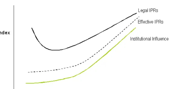
combination of institutional quality and “legal IPRs.” This is demonstrated in Figure 2.1.

So long as the positive influence of institutional improvement on IPRs exceeds any net imitative marginal benefit from decreasing IPRs as a country develops, the optimal level of

effective IPRs will always increase as a country develops.

Figure 2.1: Legal vs. Effective IPRs

Letβ ∈[0,1] represent legal IPRs in Figure 2.1 and embody the characteristics previously outlined by CP. In addition, consider a measure of institutional influenceψ∈[0,1] such that stronger institutions correspond to larger values of ψ. In other words ψ = 0 means that a

ψ= 1 means there is perfect institutional quality and all laws on the books are completely

effective. As previously stated, institutional quality will increase as a country develops. This

suggests thatψ0(θ)>0. It is also assumed that|β0(θ)|<|ψ0(θ)|, indicating that an increase in per capita GDP will have a greater marginal impact on improving institutional influence

in a country than it will have on changing the optimal level of legal IPRs.8 The functional form for the linear combination demonstrated in Figure 2.1 is represented by β+₂ψ such that 0≤ β+₂ψ ≤1 captures effective IPRs.

Distinguishing between legal IPRs and effective IPRs, as outlined above, lends to a

theoretical model that is similar in structure to that of CP. Structural differences arise in the quality of the domestically produced goods, as quality is now dependent not only on

the legal IPRs but also on the institutional influences that impact the effectiveness of these

IPRs. More specifically, in Sector A, firm F continues to supply a good of quality µF while

the quality of firm D’s good is µD(β+₂ψ, θ) = µ0+µFφ(θ)[1−α(β+₂ψ)]. The limitation to

imitation that results from stronger IPRs is now captured by α(β−ψ) such that αβ >0,

αψ >0,α0(β+₂ψ)>0, 0≤α(β+₂ψ)≤0,α(1) = 1, and 0≤µ0 ≤µF(1−φ(1)). A combination

of perfect IPR protection and perfectly effective IP laws (as identified byβ = 1 andψ= 1)

results in no imitative capabilities for firm D. Finally, as in CP, all firms in Sector A have

a constant unit cost of cA∈[0, µ0].

In Sector B, firm L now produces a good of quality v(z;θ), where z(β −ψ;θ) ≥ 0 represents firm L’s quality improvement through innovation. Firm M produces a good in

Sector B of qualityvM(β+₂ψ;θ) =v(z;θ)−γ(β+₂ψ)(v(z;θ)−v0) such that for everyθ, 0≤v0,

γ(0)>(1/vz(0, θ)), γβ >0, γψ >0,γ0(β+₂ψ) >0 and γ(1) = 1. These assumptions ensure that 0< γ(β+₂ψ)≤1, which results in a non-negative valuation ofvM. As in the CP model,

8

it is again assumed that v0≡0 and constant unit costscB≡0.

The four stages of the game remain the same as those in CP’s model: (1) the domestic

government chooses legal IPRs, (2) firm L chooses domesticR&Dexpenditures, (3) all firms

set prices, and (4) production and consumption is carried out in both sectors. Consider the

first stage for a moment, in which the domestic government chooses legal IPRs as embodied

by β. The government chooses legal IPRs given a set of ideologies regarding the decision.

These ideologies may or may not be borne out in practice. Laws are not always written to

correspond to what will necessarily happen, but rather because of what the government’s

ideologies are for making the law. This line of reasoning supports the idea that countries respond to international pressures to implementing IPRs, which will be discussed later in

the paper. For the purposes of the current theoretical model, however, it is assumed that

the government’s choice in legal IPRs reflects their ideologies for implementing the law and

does not necessarily depend on whether the law can and/or will be enforced. Therefore,

the government still chooses legal IPRs that ideally maximize social welfare (rather than

choosing effective IPRs).

Given these alterations, the prices set by firms in Stage 3 mirror those found by CP in

their functional form based on product qualities. Specifically,

SectorA     

pD _{= c}A

pF _{= µ}F _−µ

0−µFφ(θ)[1−α(β+₂ψ)] +cA

SectorB     

pM = cB;

pL= v(z;θ)γ(β+₂ψ) +cB.

The same is true for firm L’s choice inR&Dexpenditures in Stage 2. In the revised model,

the optimal level ofR&Dexpenditures satisfies the first order conditionN γ(β+₂ψ)vz−1 = 0. DefiningH=N γ(β+₂ψ)vz−1, and applying the IFT lends to the following:

zβ(β, ψ, θ) =− ∂H ∂β ∂H ∂z

=−N γβ( β+ψ

2 )vz

N γ(β+₂ψ)vzz

zθ(β, ψ, θ) =− ∂H

∂θ ∂H

∂z

=−N γ( β+ψ

2 )vzθ

N γ(β+₂ψ)vzz

>0;

zψ(β, ψ, θ) =− ∂H ∂ψ ∂H ∂z

=−N γψ( β+ψ

2 )vz

N γ(β+₂ψ)vzz

>0.

Only the result zψ(β, ψ, θ) > 0 is new. It indicates that, as expected, innovation will be

lower the weaker a country’s institutional quality.

Domestic social welfare now accounts for the institutional influence on legal IPRs.

Domestic Social Welfare (Revised Model)=µ0+µFφ(θ)[1−α(

β+ψ

2 )] +N v(z;θ)−z (2.4)

wherez(β+₂ψ;θ). The domestic government chooses legal IPRs to maximize domestic social welfare as represented in (2.4). The optimal level of IPRs satisfies

−µFφ(θ)αβ(

β+ψ

2 ) + [N vz(z(

β+ψ

2 ;θ);θ)−1]zβ(

β+ψ

2 ;θ) = 0. (2.5)

whereβ(θ) andψ(θ). In (2.5),µFφ(θ)αβ(β+₂ψ) represents the marginal cost to social welfare of increasingβand [N vz(z(β+₂ψ;θ);θ)−1]zβ(β+₂ψ;θ) represents the marginal benefit to social welfare of increasing β.

The relationship of primary interest is how the optimal level of effective IPRs (or β+₂ψ) changes as a country develops (or θincreases). Equation (2.6) embodies this effect. Notice

that the effect of an increase in per capita GDP on effective IPRs can be broken into two

components: (1) the effect of an increase in per capita GDP on legal IPRs and (2) the effect

d(β+₂ψ)

dθ =

∂(β+₂ψ)

∂β ·

dβ dθ +

∂(β+₂ψ)

∂ψ ·

dψ

dθ (2.6)

=1 2·

dβ dθ +

1 2·

dψ dθ

Since |β0(θ)|< |ψ0(θ)| the effective level of IPRs is monotonically increasing as a country develops even when the optimal legal level of IPRs is decreasing.

2.4

Linking Theory and Empirical Analysis

The revised theory provides a theoretical rationale for a monotonically increasing

rela-tionship between effective IPRs and per capita GDP. The next step is to focus on empirical

analysis of the longitudinal relationship between IPRs and per capita GDP. Before doing

so, a few comments should be made about the empirical analysis in this paper compared

to that of CP. Both this paper and CP’s paper use the Ginarte and Park IPR Index to

approximate a country’s level of IPRs. Given the opposing theories captured in Figure 2.1,

it is natural to ask whether the Ginarte and Park IPR Index best captures legal IPRs or effective IPRs. In order to answer this question, let’s first examine the Ginarte and Park

IPR Index in more detail.

2.4.1 The Ginarte-Park IPR Index

When empirically analyzing intellectual property rights, two indices for the strength of

patent systems have commonly been used. In 1990, Rapp and Rozek developed an IPR

index based on how closely a country’s patent policies mirror those embodied by US patent laws. In 1997, Ginarte and Park introduced a broader index of patent strength. Specifically,

the Ginarte-Park (GP) Index accounts for; (1) coverage, (2) membership in international

treaties, (3) loss of protection, (4) enforcement, and (5) duration of protection. Since its

IPR analysis.9 This is because the GP Index embodies a greater number of countries and years, and considers a greater scope of categories in its construction (which lends to a more

precise estimate).

This paper utilizes an updated version of the GP Index that contains data for 121

countries at five-year intervals between 1960 and 2000.10 A detailed description of the construction of the index, as outlined in Ginarte and Park (1997), can be found in Appendix

A.2. However, further analysis of the enforcement component of the GP Index provides

insight as to whether the measure is best approximating legal IPRs or effective IPRs in the

above theories.

The enforcement component of the GP index generates a dummy variable based on

whether the country (1) implements preliminary injunctions to protect the patentee until

a final decision about infringement is made by the courts, (2) protects against third party

induced infringement, and (3) implements burden-of-proof reversals to place the burden

of proving “innocence” on the individual doing the alleged infringement rather than the

patentee. It is important to justify whether or not this enforcement component is sufficient

in capturing the effective level of enforcement of IPRs in these countries. If it does, then

the GP Index measures effective IPRs in a country.

In fact, there is recent evidence to suggest that the GP Index does capture countries’

effectively enforced level of IPRs. This support is provided in a recent comparison between

the GP Index and a newly developed IPR rating created by the World Economic Forum. The

World Economic Forum released an IPR rating in their 2000 Annual Global Competitiveness

Report (GCR) that was based on surveys of opinions and experiences of firms and individuals

in an array of countries.11 Thus, the GCR Index provides information aboutperceived IPRs, 9_{For example, this is true in Maskus (2000), Schneider (2004), and Chen and Puttitanun (2005).}

10

I would like to thank Professor Walter Park for providing me with the updated index. Note that IPR data is available for 1960, 1965, 1970, 1975, 1980, 1985, 1990, 1995, and 2000.

11_{The IPR index found in the Global Competitiveness Report does not provide historical data, given that}

which implicitly includes their effective enforcement.12 Comparison of the two indices in the one year (2000) for which overlapping data is available reveals that the GCR rating

and the GP Index are strikingly similar. In fact, the indices have a positive correlation

of approximately 0.8.13 This comparison suggests that there is little difference between perceived IPRs in these countries and the level of IPRs reported by GP, thereby providing

support that the GP Index approximates effective IPRs.

If the GP Index best captures effective IPRs, then why did CP find a statistically

sig-nificant U-shape link between the GP IPR Index and per capita GDP in their empirical

analysis? The first answer to this question lies in the fact that the GP Index is an approxi-mation of effective IPRs, meaning that some errors likely exist in the index’s representation

of effective IPRs. Secondly, regional influences on the longitudinal relationship between IPRs

and per capita GDP are carefully examined in this paper and prove to play an important

role in IPR choice. These regional influences were not included in CP’s analysis.

The next section explores the longitudinal relationship, first by focusing on time series

data and then by applying what has been observed in the time series data so to better

analyze the longitudinal relationship between IPRs and per capital GDP using the entire

panel data set.

2.5

Exploring the Longitudinal Data

In general, IPRs for a given country remain the same or increase over time barring any

regime shift or other change in a country’s political economy. Only 14 out of 121 countries

show any decrease in the GP Index over time.14 In addition, only India exhibited a decrease in IPRs at a point in time when their per capita GDP was at or below the critical US$785

level, which was found to be the level of per capita GDP that corresponds with the minimum 12

The GCR Index includes patents as well as other varieties of IPRs such as copyrights and trademarks.

13

Economic Freedom of the World: 2001 Annual Report; Chapter 4.

14_{Bolivia, Brazil, Colombia, Costa Rica, Ecuador, Germany, Guatemala, Honduras, India, Malaysia,}

level of IPRs in a preliminary quadratic regression. (See Table A.2 in AppendixA.1.) The

majority of countries that demonstrate a decrease in their IPR index are middle-income

developing or already developed countries. This is an important point given that previous

theories postulate that it is the least developed countries that decrease IPRs as they grow.

Finally, ten of the fourteen countries with a decrease in IPRs over time are located in Latin

America. This fact suggests that there may be a regional effect coming into play between

IPRs and per capita GDP that may impact Latin American countries differently than the

rest of the world.15

Given the fact that only 14 out of 121 countries ever show a decrease in IPRs over time, it can be concluded that, in general, IPRs within countries remain the same or increase

over time. Since economic development is embodied by increases in per capita income

over time, the strength of IPRs for a given country would expectedly remain the same or

increase as a country develops. Time series regressions on each country largely reject the

longitudinal U-shape proposed in past literature. Time series analysis is conducted even

though a complete set of time series data contains only eight data points, which is small and

lends to questionable asymptotic properties in estimation. In order to address the problems

brought about by the small sample size in time-series analysis, a longitudinal relationship

between IPRs and per capita GDP is later examined using the entire panel data set.

When time series regressions are run on the 102 countries that have a complete set of time

series data,16 only 24 countries17 report a significant quadratic relationship between IPRs 15_{Such regional influences may implicitly appear in the theoretical model via the institutional quality}

variable. Institutional quality and institutional structure may vary between regions, resulting an a regional impact in empirical analysis. It is also possible that there are region-wide changes in the political economy for which a decrease in IPRs may result. Political economy “shocks” are not introduced into the theoretical model, but they do provide an intuitive caveat for stable or increasing IPRs as a country develops. This caveat will be emphasized throughout the paper. Nonetheless, there is not an explicit account of regional influences in the theoretical model. Therefore, the significance of regional effects found in the empirical longitudinal exploration explain more than what is presented in the theoretical model.

16_{A complete set of time series data would be data for 1965, 1970, 1975, 1980, 1985, 1990, 1995 and 2000}

as a result of limitations in the GP Index and per capita GDP data. Countries with less than the maximum number of time series data points (eight data points) are omitted.

17

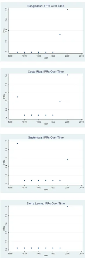
and logged per capita GDP at the 90 percent level. Only four countries–Bangladesh, Costa

Rica, Guatemala, and Sierra Leone–indicate a quadratic relationship that is significant at

the 99 percent level. The distinction in levels of significance is important as the quadratic

relationship for the entire panel data set has been consistently found at the 99 percent level

in past research.

The graphical representation of these four countries indicates that only Costa Rica and

Guatemala truly represent any downward swing in the strength of IPRs over time.

Coinci-dentally, the decrease in IPRs in 1970 corresponds with the collapse of the Central American

Common Market (CACM) of which both Costa Rica and Guatemala were members. This link is significant as the CACM established IPR guidelines for member countries. In

ad-dition, the IPR index increases in both Costa Rica and Guatemala after that CACM was

reinstated in 1991. (Costa Rica shows an increase in 1995 and Guatemala in 2000.) This

suggests that the downward longitudinal swing of IPRs in these countries is a consequence

of a shift in the political economy rather than a consequence of development.

The graphs for Sierra Leone illustrate a curious relationship. While the strength of IPRs

in Sierra Leone remains constant or increases over time, IPRs decrease with respect to per

capita GDP. This suggests that per capita GDP in Sierra Leone is decreasing over time.

When considering the complete data set, thirteen African countries exhibit the anomaly that

per capita GDP is decreasing over time.18 Each of these thirteen countries, however, either maintain or increase IPRs over time, but never decrease IPRs over time. This suggests that,

in these countries the choice in IPRs is not necessarily driven by their stage in development.

Accounting for sub-Saharan African countries in longitudinal analysis therefore becomes

very important.

While time series analysis supports the claim that individual countries generally maintain

or increase their IPRs as they develop, the small sample size is less than ideal. A maximum

of only eight data points is available for each country to analyze the time series regression

between IPRs and logged per capita GDP. As a result, methods to isolate the time-series 18

effect in the panel data provide improved asymptotic qualities of the estimators and are,

therefore, worth exploring. This will be done first by looking at the IPR-per capita GDP

relationship while pooling together countries with similar time series characteristics. Then,

using the full panel of data, the choice in IPRs will be examined in the context of a fully

specified model, where independent variables other than per capita GDP are included in the

regression equation.

2.5.1 Pooled Data Analysis of the IPR-per capita GDP relationship

Most methods to isolate time effects in panel data impose a common per capita GDP

slope coefficient for all countries. There are regional specific characteristics, which were

discussed in the previous section, that suggest slope coefficients likely vary between certain

regions. Therefore, in this study countries in regions with similar characteristics are pooled

together, and slope coefficients vary between each pooled group.

To be more specific, the entire panel data set is divided into four pooled groups. The first

group includes countries in the region of Latin America and the Caribbean. As previously

stated, ten of the fourteen countries showing a decrease in the IPR Index over time were from this region. Therefore, the pooled group of Latin America and the Caribbean will

capture the similarities in this geographical region. Countries in this region were specified

using the regional classifications of the United Nations.19

The second pooled group includes sub-Saharan African countries. Over a third of the

countries in this region exhibit a dominant downward trend in per capita GDP over time.20 Many of these countries continue to increase IPRs despite the decrease in per capita GDP.

This effect was exhibited in the graph of Sierra Leone presented in the previous section. As

with the regional classification of Latin America and the Caribbean, and the United Nations’

classification was used to identify countries to the sub-Saharan region. In this classification,

sub-Saharan Africa is designated as all of Africa except northern Africa, with the Sudan 19_{http://unstats.un.org/unsd/methods/m49/m49regin.htm.}

20_{Angola, Central African Republic, Chad, Democratic Republic of the Congo, Cote d’Ivoire, Ghana,}

included in sub-Saharan Africa.

The third pooled group consists of those countries for which there exist only two data

points: 1995 and 2000. These are mostly transitional, Eastern European economies, but also

include China and Vietnam. Specifically, only two data points are available for Bulgaria,

China, Czech Republic, Hungary, Lithuania, Poland, Romania, Russian Federation, Slovak

Republic, Ukraine, and Vietnam. It is possible that the limited time series in these countries,

as well as their sudden inclusion in 1995, at a time when IPRs were internationally on the

rise, may be skewing the panel results. The fourth and final group in the pooled analysis

includes all other countries not otherwise specified in one of the three previously mentioned groups.

Table 2.1: Group Classification used in Pooled Regression Analysis Group 1 Latin America & the Carribean

Group 2 Sub-Saharan Africa

Group 3 Transitional Economies, China, & Vietnam Group 4 All Other Countries

Note: Transitional Economies, China, & Vietnam, are countries that have a limited sample size for IPRs.

For each pooled group, an interaction term is created between per capita GDP and a

dummy variable, P OOLi, that equals 1 for each Group j = i, and zero otherwise. This

allows each pooled group to have a different slope coefficient. Countries within groups

do not necessarily have similar intercepts, however. To account for country differences

within groups, each country is given its own intercept. In addition, year fixed effects are

included to capture difference between years. (Given that the estimation finds country

specific intercepts, intercepts for each pooled group are omitted.)

IP Rkt=αk+αt+

4

X

i=1

(βilog(per capita GDPit)∗P OOLi)+

4

X

i=1

(θi[log(per capita GDPit)]2∗P OOLi) +εkt;

where,

P OOLi



 

 

= 1 if Groupj =i;

= 0 if Groupj6=i

(2.7)

whereαk is the country specific intercept term andαt is the year specific intercept term.

Results for the pooled regression are found in Table 2.2. As shown in column I, none of

the groups exhibit a significant U-shape. In fact, the coefficients on the rest of the world

(Group 4) instead tell a story more along the lines of a diminishing marginal choice in the

strength of IPRs as a country develops. This is particularly encouraging as Group 4 contains

382 of the 840 total observations in the pooled regression.

Overall, accounting for variation in slope coefficients for the four specified groups enables

the longitudinal effects in panel data to be better isolated. The results of the pooled regres-sions do not provide support for a longitudinal U-shape relationship. In the next section,

the longitudinal relationship between IPRs and per capita GDP will be examined in more

detail by considering a fully specified choice equation for IPRs.

2.6

The Fully Specified Model

The objective of the fully specified model is to account better for the variety of factors

that influence a country’s choice in IPRs. A fully specified model leads itself to a more

Table 2.2: Pooled Regression Using Panel Data

I II

Group 1 log(pc GDP) 0.32 0.27**

(0.24) (2.28)

Group 1 [log(pc GDP)]2 -0.01 (-0.07)

Group 2 log(pc GDP) 0.12 -0.02

(0.28) (-0.33)

Group 2 [log(pc GDP)]2 -0.01 (-0.34)

Group 3 log(pc GDP) -0.10 0.92***

(-0.02) (1.68)

Group 3 [log(pc GDP)]2 _0.07

(0.25)

Group 4 log(pc GDP) 0.49* 0.42*

(11.50) (33.21)

Group 4 [log(pc GDP)]2 -0.01*** (-1.69)

1970 0.02 0.02

(0.60) (0.49)

1975 0.00 -0.01

(0.04) (-0.26)

1980 0.10* 0.09*

(2.61) (2.26)

1985 0.15* 0.13*

(3.62) (3.32)

1990 0.15* 0.13*

(3.62) (3.30)

1995 0.44* 0.41*

(8.32) (8.55)

2000 0.79* 0.75*

(13.33) (14.93)

Observations 840 840

R-squared 0.9920 0.9920

2.6.1 Estimating IPRs

Numerous variables impact a country’s choice in IPRs. A country’s choice in IPRs

may depend not only on their level of development (or per capita GDP), but also on their

level of openness and institutional quality. Proxies for each of these factors are included as regressors in the IPR equation and will be discussed further in a moment. In addition, a

country’s choice in IPRs may vary depending on their regional association. Latin American

and the Caribbean, sub-Saharan Africa, and Eastern European Transitional Economies

(including China and Vietnam) are the three regions with unique links that have already

been discussed.21 Dummy variables for these regions are therefore included in the fully specified model. Finally, time fixed effects are also included so to capture variation in the

IPR choice related to a certain year. To summarize, the full specification of the IPR equation

is as follows:

IP Rit=β1log(yit) +β2[log(yit)]2+β3log(opennessit) (2.8) +β4log(institutional qualityit) +β5Latini+β6Africai+β7Transitionali+εit.

Openness

The impact of openness to trade on a country’s level of IPRs is ambiguous. It is possible

that the more open a country is to trade, the stronger IPRs will be in order to entice high

technology goods. On the other hand, greater openness may occur in hopes of imitating

high technology goods, which would result in expectedly weak IPRs.

A country’s level of openness to trade depends on such things as tariffs, quotas, and

exchange controls. However, it is difficult to measure openness in a way that is not

endoge-nous with per capita GDP. The “Freedom to Trade Internationally” Index mitigates the

possibility of endogeneity. “Freedom to Trade Internationally” is a subindex included in the 21_{China and Vietnam are included in regional classification for Transitional Economies as all these countries}

Fraser Institute’s Economic Freedom of the World Index (to be discussed in more detail in

the below section on institutional quality). “Freedom to Trade Internationally” is estimated

using equally weighted data on the following five areas: (1) taxes on international trade, (2)

regulatory trade barriers such as non-tariff barriers, (3) the actual size of the trade sector

compared to expected trade sector, (4) the difference between the official exchange rate and

the black market rate, and (5) international capital market controls. Thus, this measure of

openness captures many desirable aspects that are often difficult to quantify without using

per capita GDP.

Institutional Quality

Institutional quality is a term used to describe a country’s ability to sustain sound

economic practices given their economic and political environment. Institutional quality is

sometimes approximated using a broad measure for economic freedom. This has been the

case in past literature analyzing IPRs.

There are two widely used indices of economic freedom: (1) TheEconomic Freedom of

the World Index created by the Fraser Institute, and (2) The Index of Economic Freedom

created by the Heritage Foundation and the Wall Street Journal. Chen and Puttitanun (2005) used the former in their previous research into the U-shape. The Economic Freedom

of the World Index accounts for five different factors: (1) size of government as measured

by expenditures, taxes, and enterprizes, (2) legal structure and security of property rights,

(3) access to sound money, (4) freedom to trade internationally, and (5) regulation of credit,

labor, and business.22 The index ranges from zero to ten, with ten embodying complete economic freedom. Beginning in 1995 a measure for intellectual property right protection

was included in the calculations of group 2. Therefore, using the Economic Freedom of the

World Index as a regressor in my estimation equation would be erroneous.

In addition to having a limited data range (with data available only beginning in 1996),

the Heritage Foundation’s Index of Economic Freedom also perpetuates simultaneity with

ness, Trade, Fiscal, Freedom from Government, Monetary, Investment, Financial, Property

Rights, Freedom from Corruption, and Labor Freedom. While the Heritage Foundation is

not specific about what goes into their calculations for property rights, the sources they

use to comprise data in this category are similar to those used in the Economic Freedom

of the World Index. This fact is a red flag that using either of these two indices of

eco-nomic freedom would bias my estimates. Using an index that, in part, measures a country’s

IPRs to approximate that country’s IPRs violate the non-collinearity assumption among

independent variables.

It is now apparent that, due to the breadth of categories included in economic freedom, such a measure will likely be correlated with a country’s choice of IPRs. As a consequence,

it is better to narrow the focus of institutional quality from the wide-ranging concept of

economic freedom to those components of institutional quality that directly impact IPRs.

These include rule of law, physical property rights, and the existence of a sound business

environment.

Rule of law and physical property rights will have a clear consequence on a country’s

IPRs, but likely not the other way around. A country will only have incentive to implement

IPRs if they know such laws will be adequately enforced and not overpowered by corruption.

In addition, laws for physical property rights provide the precursor for laws for intellectual

property rights. Thus stronger physical property rights suggest the onset of stronger IPRs.

(Note, the direction of casualty is from physical property rights to IPRs.) Measures for rule

of law and physical property rights can be calculated by removing the IPR measure from

“legal structure and property rights” component of the Economic Freedom of the World

Index.

A sound business environment supports innovation and IPR related growth.23 _Without

sound business environment, firms’ ability to innovate, as well as the benefits from

innova-tion, will be stunted. Component 5 of the Economic Freedom of the World Index, which

measures the “regulation of credit, labor, and business” effectively captures the sound busi-23

ness environment critical to institutional quality. Thus, the measure of institutional quality

used in the empirical estimations of this paper combine rule of law, physical property rights,

and business environment.

2.6.2 Endogeneity of IPRs and per capita GDP

Although the key relationship of interest is how IPRs are affected by levels of per capita

GDP, the causality also works in the other direction: per capita GDP is a function of

IPRs. Countries with stronger IPRs may generate more output and lead to more economic

growth. Ginarte and Park (1997) acknowledge problems pertaining to simultaneity, but they

did not account for it in their empirical analysis. Although Chen and Puttitanun (2005) do

incorporate a two-stage regression in their evaluation of the U relationship, they estimate

IPRs in the first stage and then estimate innovation as a function of IPRs in the second

stage.

Since CP model innovation to be dependent on income levels, their endogenous

rela-tionship is similar to the simultaneity of IPRs and income used in this paper. However,

the two-stage model CP used does not account for all the possible effects that IPRs could have on income. Intellectual property protection in a country not only impacts domestic

innovation, but also affects things such as the country’s attractiveness to foreign companies.

A direct endogenous relationship between income and IPRs is therefore considered in this

paper.

In the case of simultaneous equations, the IPR equation will be estimated using a

two-stage least squares, instrumental variables approach. The next step, then, is to identify the

estimating equation for the included endogenous variable, per capita GDP.

2.6.3 Estimating per capita GDP

Per capita GDP in a given period depends upon physical capital, population, human

capital, and the level of intellectual property rights. Greater levels of physical and human

capital would expectedly lead to higher levels of output. Similarly, countries with stronger

other hand, expectedly has a negative relationship with per capita GDP. This relationship

between per capita GDP and the mentioned explanatory variables can be captured in a

traditional Cobb-Douglas production function as demonstrated below.

Yit=AitK_itα1P op_itα2H_itα3eγIP Rit

or

yit=

Yit

P opit

= AitK α1

it P op α2

it H α3

it eγIP Rit

P opit

or

log(yit) = logAit+α1logKit+ (α2−1) logP opit+α3logHit+γIP Rit+εit (2.9) whereYit= output for country i at time t;

P opit = Population;

Kit = Physical capital stock;

yit= per capita GDP;

Hit= Human capital as approximated by tertiary school enrollment rates

IP Rit= Index of IPR strength.

In the two-stage estimation, human capital is approximated by tertiary school enrollment

rates. Data on tertiary school enrollment rates is available on the UNESCO web site.24 IPR strength is approximated by the GP IPR Index discussed previously. Data on per capita

GDP (in constant 2000 US dollars) and total population are obtained from the World Bank’s

World Development Indicators (WDI). 24