Lax_unc_0153D_16082.pdf

COMBINATORIAL STRUCTURES IN THE COORDINATE RINGS

OF SCHUBERT VARIETIES

David C. Lax

A dissertation submitted to the faculty at the University of North Carolina at Chapel Hill in partial

fulfillment of the requirements for the degree of Doctor of Philosophy in the Department of

Mathematics in the College of Arts and Sciences.

Chapel Hill

2016

c

2016

David C. Lax

ABSTRACT

David C. Lax: Combinatorial Structures in the Coordinate Rings

of Schubert Varieties

(Under the direction of Robert A. Proctor)

Given an increasing sequence of dimensions, a flag in a vector space is an increasing sequence of

subspaces with those dimensions. The set of all such flags (the flag manifold) can be projectively

coordinatized using products of minors of a matrix. These products are indexed by tableaux on a

Young diagram. A basis of “standard monomials” for the vector space generated by such projective

coordinates over the entire flag manifold has long been known. A Schubert variety is a subset of

flags specified by a permutation. Lakshmibai, Musili, and Seshadri gave a standard monomial basis

for the smaller vector space generated by the projective coordinates restricted to a Schubert variety.

Reiner and Shimozono made this theory more explicit by giving a straightening algorithm for the

products of the minors in terms of the right key of a Young tableau. This dissertation uses the

recently introduced notion of scanning tableaux to give more-direct proofs of the spanning and

the linear independence of the standard monomials. This basis is a weight basis for the dual of a

Demazure module for a Borel subgroup of the general linear group.

ACKNOWLEDGEMENTS

I wish to acknowledge the UNC Department of Mathematics for providing a supportive

environ-ment for studying mathematics. Special thanks to my advisor Bob Proctor. He was extraordinarily

involved in my education. He made several notational and expositional suggestions for this

disserta-tion and alerted me to several places where more detailed proofs would be helpful. Credit for the

clarity of exposition in this document belongs to him. More special thanks to Shrawan Kumar for

sharing his immense expertise, to Matt Willis for introducing me to algebraic combinatorics, and to

Joe Seaborn for many helpful discussions. Thanks also to Michael Malahe and Ryo Moore for help

with L

_TEX.

I benefited from the financial support of the Tom Brylawski Memorial Fellowship and the

Dissertation Completion Fellowship from the University of North Carolina Graduate School for

which I am thankful.

TABLE OF CONTENTS

LIST OF FIGURES . . . .

vii

CHAPTER 1: INTRODUCTION . . . .

1

PART I:

Standard Monomial Basis for Coordinates of Schubert Varieties . . . .

3

CHAPTER 2: COORDINATES OF SCHUBERT VARIETIES . . . .

3

2.1

Introduction to Part I . . . .

3

2.2

Combinatorial tools

. . . .

6

2.3

Flags of subspaces and tabloid monomials . . . .

11

CHAPTER 3: SPANNING THEOREMS . . . .

15

3.1

Tableau monomials span Γ

. . . .

15

3.2

Demazure monomials span the Demazure quotient . . . .

21

CHAPTER 4: A LINEAR INDEPENDENCE THEOREM . . . .

26

4.1

Preferred bases and Bruhat cells

. . . .

26

4.2

Tabloid monomials, Bruhat cells, and Schubert varieties . . . .

29

4.3

Linear independence of the Demazure monomials . . . .

32

CHAPTER 5: CHARACTER FORMULAS

. . . .

37

5.1

Summation formula for Demazure polynomials . . . .

37

5.2

Contemporary terminology

. . . .

37

PART II:

Order Filter Model for Minuscule Plücker Relations . . . .

43

CHAPTER 6: MINUSCULE FLAG MANIFOLDS . . . .

42

6.1

Introduction to Part II . . . .

42

6.2

Known Results . . . .

43

6.3

Minuscule representations . . . .

47

CHAPTER 7: A MODEL FAMILY OF MINUSCULE FLAG MANIFOLDS

. .

48

7.1

Classical geometry approach . . . .

48

7.3

Concrete Lie algebra actions . . . .

53

CHAPTER 8: MINUSCULE POSETS

. . . .

56

8.1

Introduction to minuscule posets . . . .

56

8.2

Wildberger’s construction of minuscule representations . . . .

58

CHAPTER 9: EXTREME WEIGHT PLÜCKER RELATIONS . . . .

62

9.1

Representation theory setting . . . .

62

9.2

Highest weight relation . . . .

64

9.3

Rotation by Weyl group . . . .

69

9.4

Exceptional cases . . . .

80

9.5

Non-simply laced cases . . . .

84

9.6

Extreme relations in type

A

. . . .

86

9.7

Geometry appendix

. . . .

89

LIST OF FIGURES

7.2

The double-tailed diamond lattice

L

. . . .

49

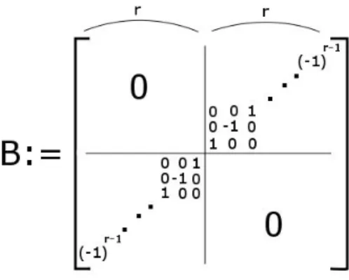
7.3

The matrix representing our bilinear form. . . .

49

7.6

A labeling of the type

D

Dynkin diagram. . . .

51

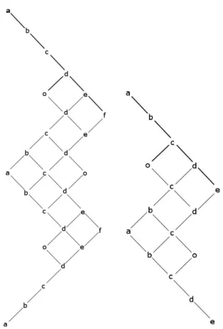
8.2

The Hasse diagrams of the minuscule posets.

. . . .

57

9.18 The colored Hasse diagrams for

e

(7) and

e

(1)

∼

=

e

(6). . . .

83

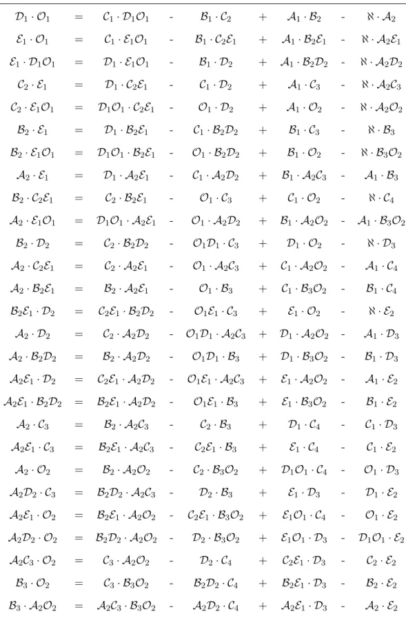
9.19 The 27 straightening laws for the complex Cayley plane on its Plücker coordinates. .

91

CHAPTER 1

Introduction

Flag manifolds and their Schubert subvarieties are fundamental geometric objects that have

algebraic realizations. In these realizations, one can study the flag manifolds through their coordinate

rings. Although we are motivated by geometry, no geometric knowledge is required of the reader.

This dissertation contains two parts, each of which concerns the coordinate rings of certain kinds of

flag manifolds or their Schubert subvarieties. Each part addresses a different question about the

coordinate rings for its special kind of manifolds. We briefly describe these two parts here: each

part contains its own more detailed introduction (Sections 2.1 and 6.1 respectively).

To specify a flag manifold, one chooses a Dynkin diagram and a subset of its nodes. To specify

an algebraic realization of this flag manifold, one then additionally chooses a dominant integral

weight whose “support” in the Dynkin diagram is the chosen subset of nodes.

express each of the vectors in the spanning set in terms of this basis.

CHAPTER 2

Coordinates of Schubert varieties

2.1

Introduction to Part I

The main results of this paper are accessible to anyone who knows basic linear algebra: the

Laplace expansion of a determinant is the most advanced linear algebra technique used. Otherwise,

the most sophisticated fact needed is that the application of a multivariate polynomial may be

moved inside a limit. Readers may replace our field

_C

with any field of characteristic zero, such as

R

.

Let

n

≥

2 and 1

≤

k

≤

n

−

1. Fix 0

< q

< q

<

· · ·

< q

< n

and let

Q

denote the set

{

q

, . . . , q

}. A

Q

-flag of

C

is a sequence of subspaces

V

⊂

V

⊂ · · · ⊂

V

⊂

C

such that dim(

V

)

=

q

for 1

≤

j

≤

k

. The set

F

`

of

Q

-flags has long been studied by geometers. It is known as a

flag manifold (for

GL

)

. Given a fixed sequence of integers

ζ1

≥

ζ2

≥ · · · ≥

ζ

with

ζ

∈

Q

for

1

≤

i

≤

m

, one can form projective coordinates for

F

`

as follows: First, any flag can be represented

with a sequence of

n

column vectors of length

n

. The juxtaposition of these vectors forms an

n

×

n

matrix

f

. For each 1

≤

i

≤

m

, form a left-initial

ζ

×

ζ

minor of

f

by selecting

ζ

of its

n

rows.

We refer to a product of such minors as a “monomial” for the given

ζ

’s. Let

N

be the number

of such possible monomials. One can inefficiently coordinatize

F

`

in

P

(

C

) by evaluating all of

these monomials over the flag manifold. The sequence

ζ

, . . . , ζ

can be viewed as the lengths of

the columns of a Young diagram

λ

. Hodge and Pedoe [1] used a basis theorem of Young [2] to index

an efficient subset of these coordinates with the semistandard Young tableaux on the diagram

λ

.

This subset is a basis of “standard” monomials for the vector space spanned by all monomials over

the flag manifold. One can group flags into subsets known as

Schubert varieties

using a form of

1

Chapters 2-5 originally appeared in the journalLinear Algebra and its Applications. The original citation is: D. C. Lax, “Accessible Proof of Standard Monomial Basis for Coordinatization of Schubert Sets of Flags,"

Linear Algebra Appl., vol. 494, pp. 105-137, 2016. DOI: 10.1016/j.laa.2016.01.003 c

Gaussian elimination on their matrix representatives; these can be indexed by

n

-permutations. For

a given Schubert variety, the coordinatization by the set of monomials indexed by semistandard

tableaux is inefficient. Utilizing recent developments in tableau combinatorics, this paper gives a

new derivation of a basis of standard monomials for the vector space generated by all monomials

restricted to a Schubert variety.

The most famous flag manifolds are the sets of

d

-dimensional subspaces of

C

. These are the

cases

k

:= 1 and

q

:=

d

above and are known as the Grassmannians. Here the basis result for

Schubert varieties may be readily deduced once it is known for the entire Grassmannian. The

next-most studied flag manifold is the “complete” flag manifold, which is the case

k

:=

n

−

1 above.

It was not until the late 1970s that Lakshmibai, Musili, and Seshadri first gave [3] a standard

monomial basis for any Schubert variety of a general flag manifold (for

GL

). Their solution used

sophisticated geometric methods and was expressed in the language of the representation theory

of semisimple Lie groups. In 1990, Lascoux and Schützenberger defined [4] the “right key” of a

semistandard tableau. In 1997, Reiner and Shimozono used the notion of right key to give [5] a new

derivation of the standard monomial basis for any Schubert variety of the complete flag manifold.

They provided a “straightening algorithm” for products of minors that expressed the monomial

specified by a given tableau as a linear combination in the standard monomial basis. In 2013, Willis

defined [6] the “scanning tableau” of a semistandard tableau and showed that it is the right key of

Lascoux and Schützenberger. The scanning tableau appears to be the simplest description of the

right key.

expression, Corollary 5.1, that is associated to the vector space at hand. It is the “Demazure

polynomial” of [7], or the “key polynomial” of [8] (which is given in terms of right keys). The

derivation of this character expression is also self-contained: In particular, the original notion of

right key is not needed.

Our spanning proof uses scanning tableaux to give a straightening algorithm in the spirit of

[5]. The determinantal identity from [9] used there is also used here; more details are given for

its application to the projective coordinates of a Schubert variety. Combinatorialists’ interest in

straightening algorithms goes back at least to [10, 11]. Apart from motivation, the spanning proof

does not need any mention of

Q

-flags or Schubert varieties. All of the necessary definitions for the

spanning theorem, Theorem 3.12, make sense for matrices with entries from any commutative ring

R

. The theorem statement itself makes sense over

R

when “spans” is replaced by “generates as an

R

-module.” The proof presented in this paper is valid at that level of generality.

Our linear independence proof follows the general inductive strategy used in [3] and [5]. However,

the simpler combinatorics of scanning tableaux allow those proofs to be simplified. One simpler

aspect is that now only single Schubert varieties need be considered in the induction, rather than

the unions of Schubert varieties that arose in the earlier papers. The statement of the linear

independence theorem, Theorem 4.15, makes sense over any field. The proof presented here is valid

for any field of characteristic zero; we make this assumption to obtain a self-contained development.

The related proof in [5] does not need characteristic zero since it refers to a standard fact concerning

the closure of a “Bruhat cell.” There it is assumed the base field is algebraically closed, but given

[12], they actually do not need that assumption for this fact. Hence the basis results in [5] and here

hold over any field. See the appendix for details.

can transition from this paper to the reductive Lie group and representation theory contexts of

references such as [13, 14]. There we describe how the standard monomial basis provides a basis of

global sections for a certain line bundle on a homogeneous space of

GL

. This is a weight basis for

the dual of a Demazure module for a Borel subgroup of

GL

. For coordinatizing Schubert varieties,

it is sufficient to consider Young diagrams with columns of length less than

n

. Such diagrams

would also suffice if one were interested only in realizing representations of

SL

. But we allow our

Young diagrams to have columns of length

n

so that we can realize all of the irreducible polynomial

representations of

GL

in the appendix.

Combinatorial tools are introduced in Section 2.2. Section 2.3 presents the definitions of flag

varieties, Schubert varieties, and their projective coordinates. Our main theorem, Theorem 2.18, is

motivated and stated there. Sections 3.1 and 3.2 prove the spanning parts of Theorems 2.16 and

2.18. Sections 4.1 and 4.2 present the facts needed to projectively coordinatize Schubert varieties.

Section 4.3 proves the linear independence parts of Theorems 2.16 and 2.18. Section 5.1 presents

the Demazure polynomial summation. Section 5.2 is the appendix of contemporary terminology.

2.2

Combinatorial tools

The needed combinatorial tools are “

Q

-chains”, which we use to index Schubert varieties, and

“tabloids”, which we use to index some projective coordinates for flag manifolds.

Fix

n

≥

2 and a nonempty subset

Q

⊆ {1

,

2

, . . . , n

−

1}

throughout the paper. Set

k

:=

|

Q

|

and index the elements of

Q

in increasing order: 1

≤

q

< q

<

· · ·

< q

< n

=:

q

. Define

[

n

] :=

{1

,

2

, . . . , n

}. A

Q-chain

is a sequence of subsets

P1

⊂

P2

⊂ · · · ⊂

P

⊆

[

n

] such that

|

P

|

=

q

for 1

≤

j

≤

k

.

An

n-partition

is an

n

-tuple

λ

= (

λ1, λ2, . . . , λ

) satisfying

λ1

≥

λ2

≥ · · · ≥

λ

≥

0 :=

λ

. Fix

an

n

-partition

λ

. The

shape

of

λ

, also denoted

λ

, is an array of

n

rows of boxes that has

λ

boxes

in row

r

. The column lengths of the shape

λ

are denoted

n

≥

ζ

≥ · · · ≥

ζ

. Denote the set of

distinct column lengths of

λ

that are less than

n

by

Q

(

λ

). Refer to a location in

λ

with column

index 1

≤

c

≤

λ

and row index 1

≤

r

≤

ζ

by (

r, c

). Sets of locations in

λ

are called

regions

. A

term

column tabloid

to refer to a tabloid of shape 1

for some

length

d

≤

n

. Given a subset

P

⊆

[

n

],

define

Y

(

P

) to be the column tabloid of length

|

P

|

filled with the values of

P

in increasing order.

There is a unique column tabloid of length

n

, namely

Y

([

n

]). A

(semistandard Young) tableau

is a

tabloid whose values weakly increase across each row. In Theorem 2.16 we use tableaux to index

the standard monomial basis for a flag manifold.

Given a

Q

-chain

π

= (

P1, . . . , P

), its

key

Y

(

π

) is the tabloid whose shape has one column each of

the lengths

q

, q

, . . . , q

and which is obtained by juxtaposing the columns

Y

(

P

)

, Y

(

P

)

, . . . , Y

(

P

)

as in Example 2.1 below. It can be seen that

Y

(

π

) is a tableau. The

Bruhat order

on

Q

-chains

is the following partial order: For two

Q

-chains

ρ

and

π

, define

ρ

π

if

Y

(

ρ

)

Y

(

π

). The

Q-carrels

for an

n

-tuple are the following

k

+ 1 sets of positions: the first

q

positions, the next

q2

−

q1

positions, and so on through the last

n

−

q

positions. To each

Q

-chain

π

, we associate the

permutation

π

of [

n

]: In

n

-tuple form, the

Q

-carrels of

π

respectively display the elements of the

k

+ 1 sets

P1, P2

\

P1, . . . , P

\

P

[

n

]

\

P

, with the elements of each set listed in increasing order.

A

Q-permutation

is a permutation of [

n

] in

n

-tuple form such that the values within each

Q

-carrel

increase from left to right. It is easy to see that the creation of

π

describes a bijection from the set

of

Q

-chains to the set of

Q

-permutations.

For 1

≤

i < j

≤

n

, define the

reflection

σ

to be the following operator on

Q

-chains: Let

π

= (

P

, . . . , P

) be a

Q

-chain. For 1

≤

`

≤

k

, form the following sets: If

i

∈

P

and

j

6∈

P

, set

P

:= (

P

\ {

i

})

∪ {

j

}. If

j

∈

P

and

i

6∈

P

, set

P

:= (

P

\ {

j

})

∪ {

i

}. Otherwise, set

P

:=

P

. It

can be seen that

P

⊂ · · · ⊂

P

; this is the

Q

-chain

σ

π

. If there exists 1

≤

`

≤

k

such that

j

∈

P

and

i

6∈

P

, then

Y

(

σ

π

) is produced from

Y

(

π

) by decreasing some values from

j

to

i

(and sorting

the resulting columns), so

σ

π

≺

π

.

Example 2.1.

Set

n

:= 7

and

Q

:=

{1

,

2

,

4}

. The chain of sets

π

:=

{5} ⊂ {3

,

5} ⊂ {1

,

3

,

4

,

5} ⊂

[7]

is a

Q-chain. Its

Q-permutation is

π

= (5; 3; 1

,

4; 2

,

6

,

7)

, where the semicolons separate the

Q-carrels

of

π. The result of the reflection

σ1

on

π

is the

Q-chain

σ1

=

{1} ⊂ {1

,

3} ⊂ {1

,

3

,

4

,

5} ⊂

[7]

.

The keys of

π

and

σ1

π

are depicted below. One can see that

σ1

≺

π.

Y

(

π

) = 1 3 5

3 5

4

5

Y

(

σ

π

) = 1 1 1

The following lemma says that we can find a reflection to step down in the Bruhat order between

two

Q

-chains:

Lemma 2.2.

Let

ρ, π

be

Q-chains. If

ρ

≺

π, then there exists

1

≤

i < j

≤

n

such that

ρ

σ

π

≺

π.

Proof.

Write

ρ

= (

R1, . . . , R

) and

π

= (

P1, . . . , P

). Find the rightmost column where the keys

Y

(

ρ

) and

Y

(

π

) differ: these columns are

Y

(

R

) and

Y

(

P

) respectively for some 1

≤

h

≤

k

. Find

the minimal

i

∈

R

\

P

and the minimal

j

∈

P

\

R

. Since

Y

(

R

)

≺

Y

(

P

), we have

i < j

. Form

the

Q

-chain

σ

π

= (

P

, . . . , P

). By the above remark

σ

π

≺

π

.

We verify that

ρ

σ

π

: For the values of 1

≤

`

≤

k

such that

P

=

P

, we have

Y

(

R

)

Y

(

P

) =

Y

(

P

). For the other values of

`

, we have

P

= (

P

\ {

j

})

∪ {

i

}. Let 1

≤

p

≤

q

denote the

row index of the value

j

in

Y

(

P

). In the rows below row

p

the value in

Y

(

P

) is the same as the

value in

Y

(

P

) since these are the values of

P

and

P

which are greater than

j

. So here the value

in

Y

(

R

) is at most the value in

Y

(

P

). For rows at and above row

p

, the value in

Y

(

R

) is at most

the value in

Y

(

P

) since

R

contains all of the

p

values of

P

which are less than

j

.

Fix an

n

-partition

λ

with

Q

(

λ

)

⊆

Q

. For 1

≤

`

≤

k

, the number of columns of length

q

in

λ

is

λ

−

λ

. The number of columns of length

n

in

λ

is

λ

. Given a

Q

-chain

π

= (

P

, . . . , P

),

its

λ-key

is the tableau

Y

(

π

) of shape

λ

obtained by juxtaposing

λ

copies of the column

Y

([

n

]),

λ

−

λ

copies of the column

Y

(

P

),

λ

−

λ

copies of the column

Y

(

P

),

. . .

and

λ

−

λ

copies of the column

Y

(

P

).

Lemma 2.3.

Let

ρ, π

be

Q-chains. If

ρ

π

, then

Y

(

ρ

)

Y

(

π

)

. When

Q

(

λ

) =

Q

the converse

holds: if

Y

(

ρ

)

Y

(

π

)

, then

ρ

π.

Proof.

Every column of length

n

is

Y

([

n

]), and every column of

Y

(

π

) of length less than

n

appears

in

Y

(

π

). When

Q

(

λ

) =

Q

, every column of

Y

(

π

) also appears in

Y

(

π

).

We now describe the scanning algorithm of [6]. Fix a sequence (

b

, b

, b

, . . .

). Define its

earliest

weakly increasing subsequence

(EWIS) to be the subsequence (

b

, b

, b

, . . .

), where

i

= 1 and for

j >

1 the index

i

is the smallest index such that

b

≥

b

. The EWIS of the sequence (6

,

6

,

4

,

3

,

5)

the EWIS, mark its location in

T

. The sequence of locations just marked is called a

scanning path

.

Fill the lowest available location of the leftmost available column of

S

(

T

) with the last member

of the EWIS. Iterate this process as if the marked locations are no longer part of

T

. Using the

row condition on the filling of

T

, it can be seen that at each stage the unmarked locations form

the shape of some

n

-partition. This implies that every location in

T

is marked once the leftmost

column of

S

(

T

) has been filled. To find the values of the next column of

S

(

T

):

1. Ignore the leftmost column of

T

and

λ

.

2. Remove the marks from the remaining locations.

3. Repeat the above process.

Continue until the shape has been completely filled with values: this is the scanning tableau

S

(

T

)

of

T

. For a location (

r, c

)

∈

λ

, let

P

(

T

;

r, c

) denote the scanning path found to fill location (

r, c

) of

S

(

T

).

Example 2.4.

Set

n

:= 6

,

Q

:=

{1

,

2

,

4

,

5}

, and

λ

:= (5

,

3

,

2

,

2

,

1

,

0)

. Below are shown a tableau

T

,

its scanning tableau

S

(

T

)

, and a figure using different symbols to depict the scanning paths found

while filling the leftmost column of

S

(

T

)

.

T

= 1 1 2 3 5

2 3 4

3 4

5 6

6

S

(

T

) = 2 2 3 5 5

3 3 5

4 5

5 6

6

• • • ♦ ♥

♦ ♦ ♠

♠ ♠

♥ ♣

♣

We need four lemmas concerning the scanning tableau

S

(

T

) of a tableau

T

of shape

λ

. Only

the first is needed to prove Theorem 3.12, the main spanning theorem. The other three along with

Lemmas 2.2 and 2.3 are used in Sections 4.2 and 4.3.

Lemma 2.5.

Let

1

≤

c

≤

λ1

and

1

≤

r

≤

ζ

−

1

. For any location

(

p, b

)

in the scanning path

P

(

T

;

r, c

)

, there exists a location

(

u, v

)

in the previous scanning path

P

(

T

;

r

+ 1

, c

)

such that

v

≤

b

and

T

(

u, v

)

> T

(

p, b

)

.

First, suppose (

p, b

) is a column bottom of

T

. The location (

p, b

) is not in

P

(

T

;

r

+ 1

, c

), but it

does belong to the sequence of column bottoms of

T

which is scanned to form

P

(

T

;

r

+ 1

, c

). Hence

its value

T

(

p, b

) was not in that previous earliest weakly increasing subsequence. Therefore there is

a column bottom (

u, v

) of

T

in the scanning path

P

(

T

;

r

+ 1

, c

) strictly to the left of (

p, b

) such

that

T

(

u, v

)

> T

(

p, b

).

Now suppose (

p, b

) is not a column bottom of

T

. Since (

p, b

) is scanned in the formation of

P

(

T

;

r, c

), the location (

p

+ 1

, b

) was marked as part of the previous scanning path

P

(

T

;

r

+ 1

, c

).

By the column strict condition on tabloids, its value satisfies

T

(

p

+ 1

, b

)

> T

(

p, b

). Take

u

:=

p

+ 1

and

v

:=

b

.

Lemma 2.6.

Every value in the rightmost column of

T

appears in every column of

S

(

T

)

. In

particular, the rightmost column of

S

(

T

)

is the rightmost column of

T.

Proof.

Fix a column index 1

≤

c

≤

λ

. As was noted above, every location in

T

to the right of

column

c

is marked in the construction of column

c

of

S

(

T

). So every location in the rightmost

column of

T

belongs to a scanning path

P

(

T

;

r, c

) for some 1

≤

r

≤

ζ

. These locations must be the

end of their respective scanning paths.

Let

λ

denote the partition obtained from

λ

by omitting the rightmost column of its shape. Given

a tableau

T

of shape

λ

, let

T

denote the tabloid of shape

λ

obtained by omitting the rightmost

column of

T

.

Lemma 2.7.

Deleting the rightmost column both before and after forming the scanning tableau, we

find that

S

(

T

)

[

S

(

T

)]

.

Proof.

Let (

r, c

)

∈

λ

. In the two applications of the scanning algorithm, the same locations are

marked and removed from within the region

λ

⊂

λ

of

T

as are from

T

. So the scanning path

P

(

T

;

r, c

) is the path

P

(

T

;

r, c

) with at most one location appended from the rightmost column of

T

. Since the values within a scanning path weakly increase, the value at the end of

P

(

T

;

r, c

) is less

than or equal to the value at the end of

P

(

T

;

r, c

). The value at location (

r, c

) in

S

(

T

) is the value

at the end of

P

(

T

;

r, c

), and the value at (

r, c

) in

S

(

T

) is the value at the end of

P

(

T

;

r, c

).

Definition 2.8.

A tableau

T

of shape

λ

is

π-Demazure

if its scanning tableau satisfies

S

(

T

)

Y

(

π

).

In Theorem 2.18 we use

π

-Demazure tableaux to index the standard monomial basis for the

Schubert variety indexed by

π

.

Lemma 2.9.

If a tableau

T

of shape

λ

is

π-Demazure, then the tableau

T

of shape

λ

is

π-Demazure.

Proof.

By the previous lemma, we have

S

(

T

)

[

S

(

T

)]

[

Y

(

π

)]

=

Y

(

π

).

2.3

Flags of subspaces and tabloid monomials

We now introduce the main objects of the paper: flags of subspaces, Bruhat cells, Schubert

varieties, and tabloid monomials. For Sections 3.1 and 3.2, only the definitions concerning tabloid

monomials are needed. Along the way we mention five facts about these structures for motivation

which are formally stated and proved in Sections 4.1 and 4.2. Our main result, Theorem 2.18, is

stated at the end of this section.

Definition 2.10.

A

Q-flag

of

_C

is a sequence of subspaces

V

⊂

V

⊂ · · · ⊂

V

⊂

C

such that

dim(

V

) =

q

for 1

≤

j

≤

k

.

We denote the set of

Q

-flags in

C

by

F

`

. An ordered basis (

v1, v2, . . . , v

) of column vectors

for

_C

_{is presented in this paper as the}

_n

_×

_n

_{invertible matrix [}

_v

1

, v

, . . . , v

] whose columns from

left to right are

v

, . . . , v

. Define a map Φ

from the ordered bases for

C

to

F

`

by sending an

ordered basis

f

:= [

v

, . . . , v

] to the

Q

-flag Φ

(

f

) of subspaces

V

=span({

v

|

i

≤

q

}) for 1

≤

j

≤

k

.

Any

Q

-flag can be represented in this way by many ordered bases. Special

Q

-flags can be made

using the axis basis vectors

e

, . . . , e

for

C

: For each

Q

-chain

π

= (

P

, P

,

· · ·

, P

), construct the

Q-chain flag

ϕ

(

π

) of subspaces

V

:=span({

e

|

i

∈

P

}) for 1

≤

j

≤

k

. Given a

Q

-chain

π

, form the

Q

-permutation

π

as in Section 2.2. Define the

n

×

n

matrix

s

to be the permutation matrix whose

(

π

, j

) entry is 1 for 1

≤

j

≤

n

. It is clear that

ϕ

(

π

) = Φ

(

s

), when

s

is viewed as an ordered

basis.

Let

B

denote the subgroup of upper triangular matrices within

GL

, the group of invertible

matrices.

We will see (Fact 4.8) that every

Q

-flag belongs to a unique Bruhat cell. The following disjoint

unions of Bruhat cells are important subsets of

F

`

:

Definition 2.12.

Let

π

be a

Q

-chain. We define the

Schubert variety

X

(

π

) to be the union of cells

ρπ

C

(

ρ

).

Our goal is to develop a coordinatization of

F

`

. Recall that projective space

P

(

C

) is the set of

lines through the origin in

_C

_{; hence it is the set}

_F

_`

{1}

of

{1}-flags. The set

P

(

C

) does not have global

coordinates in the usual (affine) sense. But it can be coordinatized by

projective coordinates

: A point

L

∈

_P

(

_C

) is indexed by an equivalence class [(

p

, p

, . . . , p

)] of

n

-tuples, where (

p

, p

, . . . , p

)

∈

C

is a nonzero point on the line

L

and two

n

-tuples (

p

, p

, . . . , p

) and (

p

, p

, . . . , p

) are equivalent

if there is a nonzero

α

∈

_C

such that (

p

, p

, . . . , p

) = (

αp

, αp

, . . . , αp

).

From now on, fix an

n

-partition

λ

such that

Q

(

λ

)

⊆

Q

. Now we begin to form projective

coordinates for

F

`

from tabloids of shape

λ

. Let

C

[

x

] denote the ring of polynomials in the

n

coordinates of a sequence of

n

vectors from

C

. Fix 1

≤

p

≤

n

. Let

f

be an

n

×

n

matrix. For any

1

≤

q

≤

n

, define the

q-initial submatrix of

f

with rows

r

, . . . , r

to be the

p

×

q

matrix whose

i

row consists of the first

q

entries of the

r

row of

f

. When

p

=

q

, in

_C

[

x

] we form for

f

its

q-initial

minor with rows

r

, . . . , r

: this is the determinant of its

q

-initial submatrix with rows

r

, . . . , r

.

Definition 2.13.

Let

T

be a tabloid of shape

λ

. For each column index 1

≤

c

≤

λ1

, form in

C

[

x

] the

ζ

-initial minor with indices

T

(1

, c

)

, . . . , T

(

ζ

, c

). The

monomial

of

T

, denoted by the

corresponding Greek letter

τ

, is the product of these minors. Let

π

be a

Q

-chain. In particular, the

monomial of the

λ

-key

Y

(

π

) is denoted

ψ

(

π

).

Example 2.14.

Set

n

:= 4

and

Q

:=

{1

,

2

,

3}

and

λ

:= (5

,

2

,

1

,

0)

. Form the tableau

T

:= 1 1 1 2 4

2 3

4

.

is the following product:

τ

=

det

             

x

y

z

x

y

z

x

y

z

             

det

x1

y1

x3

y3



det

([

x1

])

det

([

x2

])

det

([

x4

])

.

Let

F

be a

Q

-flag. We will see (Lemma 4.9) that the sequence of the valuations of all tabloid

monomials of shape

λ

on the ordered bases for

F

is projectively well defined: Varying the choice of

basis

f

such that Φ

(

f

) =

F

will scale all these values equally. We will also see (Fact 4.14) that

when

Q

(

λ

) =

Q

, this sequence of monomials give a faithful projective coordinatization of the set

F

`

of

Q

-flags.

Definition 2.15.

Let Γ

denote the vector subspace of polynomials in

_C

[

x

] that are linear

combinations of the tabloid monomials of shape

λ

.

While it is useful to consider the set of all tabloid monomials, the following long-known result

shows that that set is much larger than is needed to span Γ

:

Theorem 2.16.

Let

λ

be an

n-partition. The monomials of the semistandard tableaux of shape

λ

form a basis of the vector space

Γ

.

Such monomials are called

tableau monomials

. The spanning and linear independence parts of

this basis theorem are reproved here as Theorem 3.8 and Corollary 4.16. This theorem implies that

when

Q

(

λ

) =

Q

, the sequence of tableau monomials gives an efficient coordinatization of

F

`

.

Now we return to having a

Q

-chain

π

fixed, as at the end of Section 2.2. Again form its

λ

-key

Y

(

π

). Define the subspace

Z

(

π

)

⊆

Γ

to be the span of the monomials of tabloids

T

such that

T

6

Y

(

π

).

Definition 2.17.

Let

π

be a

Q

-chain. The

Demazure quotient

for

π

is the vector space Γ

(

π

) :=

Γ

/Z

(

π

).

We will see (Lemma 4.11) that all tabloid monomials in

Z

(

π

) are zero on the Schubert variety

“monomial” to refer to the residue of a monomial in Γ

(

π

). Since the set of tableau monomials is now

much larger than is needed to span Γ

(

π

), we need an analog of Theorem 2.16 for the space Γ

(

π

).

Our main result is a new proof of the following theorem that is based on the scanning tableaux

S

(

T

):

Theorem 2.18.

Fix a nonempty

Q

⊆

[

n

−

1]

. Let

λ

be an

n-partition such that

Q

(

λ

)

⊆

Q

and let

π

be a

Q-chain. The monomials of the

π-Demazure tableaux of shape

λ

form a basis of the vector

space

Γ

(

π

)

.

Such monomials are called

π-Demazure monomials

. The spanning and linear independence

parts of this basis theorem are Theorem 3.12 and Theorem 4.15. This theorem implies that when

CHAPTER 3

Spanning Theorems

3.1

Tableau monomials span

Γ

Before we prove the spanning part of our main result, Theorem 2.18, in the next section, we

must first prove the spanning of Γ

by tableau monomials in Theorem 2.16. We begin by presenting

a translation of a classical determinantal identity into the language of tabloid monomials. This is a

“master” identity that we use in two ways to prove the two spanning results by establishing relations

amongst certain monomials. The idea of both proofs is the same: Using a total order on the set

of tabloids, we provide straightening algorithms for applying the master identity. Each use of the

identity progresses in the same direction under this order. The control afforded by the total order

implies the termination of the algorithm. This is a common strategy; it was also used in [5].

Fix an

n

-partition

λ

; the sets

Q

and

Q

(

λ

) play no role in this section. Fix a tabloid

T

of shape

λ

and a region

µ

⊆

λ

. The region

µ

selects which locations are “active” in the master identity. The

multiset of values of

T

within

µ

is denoted

T

(

µ

). For 1

≤

j

≤

λ

, let

T

denote column

j

of

T

and

let

µ

denote the intersection of

µ

with column

j

of

λ

. Let ¯

µ

denote the region of

λ

complementary

to

µ

.

Definition 3.1.

A

µ-shuffle of

T

is a permutation of the values of

T

that can be obtained by the

composition of two permutations as follows: First permute the values within the region

µ

such

that the values within a given column are distinct. Then sort the values within each column into

ascending order to obtain a tabloid.

Given a

µ

-shuffle

σ

of

T

, the resulting tabloid is denoted

T

and its monomial is denoted

τ

.

Let

(

σ

) denote the sign of

σ

as a permutation. For a tabloid

T

with repeated values, it is possible

that for

µ

-shuffles

σ

6=

σ

of

T

we have

T

=

T

.

We prepare to construct a square compound matrix

M

(

T

) based on

T

and

µ

. Let

g

be the

minors in

g

form the monomial

τ

of

T

into two rectangular parts. The next two definitions are

illustrated at j = 1 in the example below. For each 1

≤

j

≤

λ

form the

ζ

× |

µ

|

“active” matrix

A

by transposing the

ζ

-initial submatrix of

g

whose rows are specified by the values of

T

(

µ

).

Also form the

ζ

× |¯

µ

|

“inactive” matrix

N

by transposing the

ζ

-initial submatrix of

g

similarly

specified by the values of

T

(¯

µ

). The total number of columns in

A

and

N

is

|

µ

|

+

|¯

µ

|

=

ζ

. Let

A

t

N

denote the

ζ

×

ζ

concatenation of the matrices

A

and

N

. Except for the order of its

columns, the matrix

A

t

N

is the transpose of the

ζ

-initial submatrix specified by the column

T

.

So its determinant is the monomial

τ

of

T

, up to a sign. These

ζ

×

ζ

matrices form the main

diagonal blocks of the compound matrix

M

(

T

).

Now in addition let 1

≤

i

≤

λ

. Form the rectangular matrix

A

by transposing the

ζ

-initial

submatrix of

g

whose rows are specified by the values of

T

(

µ

). Then let

A

t

0 denote the

ζ

×

ζ

concatenation of the matrix

A

with a

ζ

× |

µ

¯

|

zero matrix. These

ζ

×

ζ

matrices form the

off-diagonal blocks of the compound matrix

M

(

T

).

Define the matrix

M

(

T

) to be the (

ζ1

+

· · ·

+

ζ

)-square compound matrix whose

j

th

_diagonal

block is

A

t

N

and whose non-diagonal block in the (

i, j

) block position is

A

t

0:

M

(

T

) :=

A

t

N1

A

t

0

· · ·

A

t

0

A

t

0

A

t

N

· · ·

A

t

0

..

.

..

.

..

.

..

.

A

1

t

0

A

<λ1>

2

t

0

· · ·

A

<λ1>

λ1

t

N

Example 3.2.

Set

n

:= 4

and

λ

:= (5

,

2

,

1

,

0)

. Use the tableau

T

and the notation of Example 2.14,

and let

µ

⊂

λ

be the region indicated by dots in the second figure:

T

:= 1 1 1 2 4

2 3

4

•

•

•

In the first column of

T

the value

4

lies in the region

µ, while the values

1

and

2

do not. Hence the

first “active” matrix is

A1

=

, and the first “inactive” matrix is

N1

=

x1 x2

y1 y2

z1 z2     

matrix

M

(

T

)

is:

x4 x1 x2 x3 0 0 x2 0

y4 y1 y2 y3 0 0 y2 0

z4 z1 z2 z3 0 0 z2 0

x4 0 0 x3 x1 0 x2 0

y4 0 0 y3 y1 0 y2 0

x4 0 0 x3 0 x1 x2 0

x4 0 0 x3 0 0 x2 0

x4 0 0 x3 0 0 x2 x4                      

The following lemma is our master identity. It says that

|

M

(

T

)|

is a polynomial in Γ

. It is

the translation hinted at by Reiner and Shimozono of the left side of the determinantal identity

(III.11) in [9] that they use as the left side of equation (5.3) in [5] . Note that the product of the

determinants of the diagonal blocks of

M

(

T

) is the monomial

τ

, up to a sign. This sign is the sign

ambiguity in the statement of the lemma. This ambiguity vanishes in our applications.

Lemma 3.3.

Let

T

be a tabloid of shape

λ

and let

µ

⊆

λ. The determinant

|

M

(

T

)|

is, up to sign,

the signed sum of monomials

(

σ

)

τ

,

where the sum runs over all

µ-shuffles

σ

of

T.

Proof.

We calculate

|

M

(

T

)|

by an iterated Laplace expansion process. We then show that the

nonzero terms in this expansion correspond to the

µ

-shuffles of

T

. Begin to calculate

|

M

(

T

)|

by Laplace expansion on the first

ζ

rows, which form the first row of blocks. This expresses the

determinant as the sum of the products of

ζ1

×

ζ1

“primary” minors and (

ζ2

+

· · ·

+

ζ

)-square

“complementary” minors.

Most of the products in this sum vanish because one of the two minors has a zero column or

because the primary minor has repeated columns. Fix a summand that does not vanish for either

of these reasons. (We allow the complementary minor to have repeated columns; the vanishing

of such a minor appears as cancellation in the summation in the lemma statement.) Since the

complementary minor at hand cannot have a zero column, its primary minor must include all of

the columns of

N

. The primary minor’s other columns come from various

A

blocks. Recall

that the columns of

N1

are the initial segments of the rows of

g

indexed by the values of

T1

(¯

µ

)

and that the columns of

A

are the initial segments of the rows of

g

indexed by the values of