Multi-Relational Data Mining

(1)

(met een samenvatting in het Nederlands)

Proefschrift

Ter verkrijging van de graad van doctor Aan de Universiteit Utrecht

Op gezag van de Rector Magnificus, Prof. Dr. W.H. Gispen, Ingevolge het besluit van het College voor Promoties

In het openbaar te verdedigen op maandag 22 november 2004 des morgens te 10:30 uur

Door

(2)

2

promotor: Prof. dr. A.P.J.M. Siebes

Faculteit Wiskunde en Informatica, Universiteit Utrecht

SIKS Dissertation Series No. 2004-15

The research reported in this thesis has been carried out under the auspices of SIKS, the Dutch Graduate School for Information and Knowledge Systems.

(3)

Acknowledgements

As is customary for a Ph.D. thesis, the road towards completion of this text has been long. Two people have been instrumental in reaching the end successfully, and getting me started in the first place. I am very grateful to Pieter Adriaans for convincing me that my research ideas were a suitable basis for a dissertation, and that getting a degree was a mere formality and would be a matter of one or two years (a slight underestimate). Equal praise to my supervisor Arno Siebes, for supporting my ideas, having the patient conviction all would end well, and letting me do things my way. Whenever my research led me off the beaten track of mainstream Data Mining, he encouraged me to press on.

I would also like to thank my colleagues at the Large Distributed Databases (read ‘Data Mining’) group at Utrecht University, who, for obscure reasons, tended to come up with Spanish nicknames, ranging from Arniño to Pensionado. In particular Lennart Herlaar, Rainer Malik and Carsten Riggelsen were of great help in getting the document printer-ready. Ad Feelders, also at the LDD group, devoted his time reading through an early draft. I hope this was as beneficial to him as it was to me.

A greatly appreciated effort was done by Kathy Astrahantseff, who checked the manuscript for typos and bad phrasing. Thanks a lot for spending so much time crossing the t’s and dotting the last

ı’s.

The person with probably the most visible impact on the book as you are currently holding it is Lieske Meima, who spent lots of here valuable spare time designing the cover and taking wonderful pictures.

(8)

8

Although at the end of the day, every letter in this thesis was conceived by me, a surprisingly small fraction of these letters was actually typed in person. Many thanks to Karin Klompmakers, Tiddo Evenhuis and Hans van Kampen for typing out endless pages of manuscript and sitting down with me to make corrections and draw tables and diagrams.

I want to express my gratitude to the members of the reading committee, Jean-François Boulicaut, Luc De Raedt, Peter Flach, Joost Kok and Hannu Toivonen, for voluntarily spoiling their summer carefully reading the manuscript and approving its publication.

Thanks also to my two assistants at the public defence of this thesis, Marc de Haas and Leendert van den Berg. Looking like a clown is best done in teams.

The following institutions have supported or contributed to the research reported in this thesis: Perot Systems Nederland B.V., the CWI (the Dutch national research laboratory for mathematics and computer science), the Telematica Institute, Utrecht University and Kiminkii.

Finally I have to mention my dad, Freerk Knobbe, who provided a lot of technical support and still recognizes randomly located paragraphs he claims to have typed. On many occasions, he helped out with tedious jobs such as creating an index or editing formulae in Word. His only complaint was that the randomness of his contributions prevented him from seeing the big picture and understanding the ‘plot’. I guess with the present dissertation in print, he will have to read it start to finish.

But all the technical and scientific support would have been in vain if it hadn’t been for the moral support provided by my friends and family, in particular my parents.

(9)

1 Introduction

This thesis is concerned with Data Mining: extracting useful insights from large and detailed collections of data. With the increased possibilities in modern society for companies and institutions to gather data cheaply and efficiently, this subject has become of increasing importance. This interest has inspired a rapidly maturing research field with developments both on a theoretical, as well as on a practical level with the availability of a range of commercial tools. Unfortunately, the widespread application of this technology has been limited by an important assumption in mainstream Data Mining approaches. This assumption – all data resides, or can be made to reside, in a single table – prevents the use of these Data Mining tools in certain important domains, or requires considerable massaging and altering of the data as a pre-processing step. This limitation has spawned a relatively recent interest in richer Data Mining paradigms that do allow structured data as opposed to the traditional flat representation.

Over the last decade, we have seen the emergence of Data Mining techniques that cater to the analysis of structured data. These techniques are typically upgrades from well-known and accepted Data Mining techniques for tabular data, and focus on dealing with the richer representational setting. Within these techniques, which we will collectively refer to as Structured Data Mining techniques, we can identify a number of paradigms or ‘traditions’, each of which is inspired by an existing and well-known choice for representing and manipulating structured data. For example, Graph Mining deals with data stored as graphs, whereas Inductive Logic Programming builds on techniques from the logic programming field. This thesis specifically focuses on a tradition that revolves around relational database theory: Multi-Relational Data Mining (MRDM).

(10)

10

normalisation may help to properly approach an MRDM project, and guide the effective and efficient search for interesting knowledge in the data. Recent developments in dealing with extremely large databases and managing query-intensive analytical processing will aid the application of MRDM in larger and more complex domains.

To a degree, many concepts from relational database theory have their counterparts in other traditions that have inspired other Structured Data Mining paradigms. As such, MRDM has elements that are variations of those in approaches that may have a longer history. Nevertheless, we will show that the clear choice for a relational starting point, which has been the inspiration behind many ideas in this thesis, is a fruitful one, and has produced solutions that have been overlooked in ‘competing’ approaches.

1.1 Data

Mining

The primary ingredient of any Data Mining [20, 33, 43, 118, 120] exercise is the database. A

database is an organised and typically large collection of detailed facts concerning some domain in the outside world. The aim of Data Mining is to examine this database for regularities that may lead to a better understanding of the domain described by the database. In Data Mining we generally assume that the database consists of a collection of individuals. Depending on the domain, individuals can be anything from customers of a bank to molecular compounds or books in a library. For each individual, the database gives us detailed information concerning the different characteristics of the individual, such as the name and address of a customer of a bank, or the accounts owned.

When considering the descriptive information, we can select subsets of individuals on the basis of this information. For example we could identify the set of customers younger than 18. Such intensionally defined collections of individuals are referred to as subgroups. While considering different subgroups, we may notice that certain subgroups have characteristics that set them apart from other subgroups. For instance, the subgroup ‘age under 18’ may have a negative balance on average. The discovery of such a subgroup will lead us to believe that there is a dependency

between age and balance of a customer. Therefore, a methodical survey of potentially interesting subgroups will lead to the discovery of dependencies in the database. Clearly, a good definition of the nature of the dependency (e.g. deviating average balance) is essential to guide the search for interesting subgroups. Such a statistical definition is known as an interestingness measure or score function.

Interesting subgroups are a powerful and common component of Data Mining, as they provide the interface between the actual data in the database and the higher-level dependencies describing the data. Some Data Mining algorithms are dedicated to the discovery of such interesting subgroups. However, interesting subgroups are a limited means of capturing knowledge about the database, because by definition they only describe parts of the database. Most algorithms will therefore regard interesting subgroups not as the end product, but as mere building blocks for comprehensive descriptions of the existing regularities. The structures that are the aim of such algorithms are known as models, and the actual process of considering subgroups and laboriously constructing a complete picture of the data is therefore often referred to as modelling.

(11)

the behaviour of new individuals. Consider, for example, a sample of customers of a bank and how they responded to a certain offer. We can build a model describing how the response depends on different characteristics of the customers, with the aim of predicting how other customers will respond to the offer. A lot of time and effort can thus be saved by only approaching customers with a predicted interest.

1.2 Propositional Data Mining

An important formalism in Data Mining is known as Propositional Data Mining. The main assumption is that each individual is represented by a fixed set of characteristics, known as

attributes. Individuals can thus be thought of as a collection of attribute-value pairs, typically stored as a vector of values. In this representation, the central database of individuals becomes a table: rows (or records) correspond to individuals, and columns correspond to attributes. The algorithms in this formalism will typically employ some form of propositional logic to identify subgroups, hence the name Propositional Data Mining.

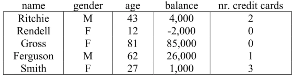
Example 1.1 Consider again the customers of a bank. Each individual can be characterised by personal information, such as name, gender and age, as well as by bank-related information such as

balance, nr. credit cards, etc. Figure 1.1 gives an example database in tabular form. Propositional algorithms typically build models by considering subgroups identified by constraints on the propositional data, e.g. ‘the group of male customers who own more than one credit card’ or ‘the adults’.

name gender age balance nr. credit cards

Ritchie M 43 4,000 2

Rendell F 12 -2,000 0

Gross F 81 85,000 0

Ferguson M 62 26,000 1

Smith F 27 1,000 3

Figure 1.1 A propositional database.

Due to its straightforward structure, the Propositional Data Mining paradigm has been extremely popular, and is in fact the dominant approach to analysing a database. A wide range of techniques has been developed, many of which are available in commercial form. In terms of designing Data Mining algorithms, the propositional paradigm has a number of advantages that explain its popularity:

• Every individual has the same set of attributes. An individual may not have a value for a particular attribute (i.e. have a NULL-value), but at least it makes sense to inquire about that particular attribute. Also, each attribute only appears once, and has a single value.

• Individuals can be thought of as points in an n-dimensional space. Distance measures can be used to establish the similarity between individuals. Density estimation techniques can be used to help discover interesting regions of the space.

(12)

12

• The meta-data describing the database is simple. This meta-data is used to guide the search for interesting subgroups, which in Propositional Data Mining boils down to adding propositional expressions on the basis of available attributes.

There is a single, yet essential disadvantage to the propositional paradigm: there are fundamental limitations to the expressive power of the propositional framework. Objects in the real world often exhibit some internal structure that is hard to fit in a tabular template. Some typical situations where the representational power of Propositional Data Mining is insufficient are the following:

• Real world objects often consist of parts, differing in size and number from one object to the next. A fixed set of attributes cannot represent this variation in structure.

• Real-world objects contain parts that do not differ in size and number, but that are unordered or interchangeable. It is impossible to assign properties of parts to particular attributes of the individual without introducing some artificial and harmful ordering.

• Real-world objects can exhibit a recursive structure.

1.3 Structured Data Mining

The Propositional Data Mining paradigm has been popular because of the simple tabular structure it proposes. This property is, at the same time, its weakness. Many databases, especially of large industrial nature, are simply too complex to analyse with a propositional algorithm without ignoring important information. Rather than working with individuals that can be thought of as vectors of attribute-value data, we will have to deal with structured objects that consist of parts that may be connected in a variety of ways. Data Mining algorithms will have to consider not only attribute-value information concerning parts (which may be absent), but also important information concerning the presence of different types of parts, and how they are connected.

active inactive

NH₂ N H N NH₂ N H N C H₃ Histamine N H N H N

CH₃ NH2

O N

Figure 1.2 A database of Histamine-related compounds.

Example 1.2 The chemical compound Histamine is a neuro-transmitter that regulates a number of processes in the human body, such as the activity of the heart and acid secretion in the stomach [90]. Histamine and variations thereof work because they bind to specific configurations of amino acids known as Histamine H2-receptors. For a compound to bind to the H2-receptor (to be active), it

(13)

Figure 1.2 shows a database of four compounds, two of which are active, and two of which inactive. A typical Data Mining exercise would aim to explain the difference in activity based on the structural properties. Clearly, the chemicals will be poorly represented in a single table and Propositional Data Mining algorithms are difficult to apply. A more sophisticated representation and analysis scheme would consider the structure and would, for example, discover fragments of compound that can form discriminative rules. For example an HN–CH fragment occurs in all positive, and none of the negative cases.

Although a range of representations for structured data has been considered in the literature, structured individuals can conceptually be thought of as annotated graphs. Nodes in the graphs correspond to parts of the individual. A node can typically be of a class, selected from a predefined set of classes, and will have attributes associated with it. Available attributes depend on the class. For example, a molecule will consist of atoms and bonds (the classes), and each class will have a different set of attributes, such as element and charge for atoms, and type for bonds. The edges in the graph represent how parts are connected.

We refer to the class of techniques that support the analysis of structured objects as Structured Data Mining. These techniques differ from alternative techniques, notably propositional ones, in the representation of the individuals and of the discovered models. Many of the concepts of Data Mining are relatively representation-independent, and can therefore be generalised from Propositional Data Mining. For example, individuals and interesting subgroups play the same role. What is different is the definition of subgroups in terms of structural properties of the individuals. Much of the remainder of this thesis is dedicated to finding good ways of upgrading powerful concepts and techniques from Propositional Data Mining to the richer structured paradigm.

Structured Data Mining deals with a number of difficulties that translate from the advantages of Propositional Data Mining listed in the previous section:

• Individuals do not have a clear set of attributes. In fact, individuals will typically consist of parts that may be queried for certain properties, but parts may be absent, or appear several times, making it harder to specify constraints on individuals. Furthermore, it will be necessary to specify subgroups on the basis of relationships between parts, or on groups of parts.

• Individuals cannot be thought of as points in an n-dimensional space. Therefore, good distance measures cannot be defined easily.

• Complementary subgroups can not be obtained by simply taking complementary values for certain properties, such as attributes of parts. For example, the set of molecules that contain a C-atom and the set of molecules that contain an H-atom are not disjoint. The different values for an attribute of a part (atom) can not be used to partition the individuals (molecules).

• The meta-data describing the database is extensive. Typically, the meta-data will not only describe attributes of the different parts, but also in general terms how parts relate to each other, i.e. what type of structure can be expected. Good Structured Data Mining algorithms will use this information to effectively and efficiently traverse the search space of subgroups and models.

(14)

14

• Graph Mining [19, 48, 79, 80] The database consists of labelled graphs, and graph matching is used to select individuals on the basis of substructures that may or may not be present.

• Inductive Logic Programming (ILP) [9, 11, 12, 13, 14, 22, 28, 30, 31, 70, 83, 89] The database consists of a collection of facts in first-order logic. Each fact represents a part, and individuals can be reconstructed by piecing together these facts. First-order logic (often Prolog) can be used to select subgroups.

• Semi-Structured Data Mining [1, 8, 16, 81, 104] The database consists of XML-documents, which describe objects in a mixture of structural and free-text information.

• Multi-Relational Data Mining (MRDM) [7, 31, 53, 59, 61, 62, 63, 74, 107] The database consists of a collection of tables (a relational database). Records in each table represent parts, and individuals can be reconstructed by joining over the foreign key relations between the tables. Subgroups can be defined by means of SQL or a graphical query language presented in Chapter 4.

In Chapter 2 we will examine Structured Data Mining in depth, and compare the four categories of techniques according to how they approach different aspects of structured data.

1.4 Multi-Relational Data Mining

The approach to Structured Data Mining that is the main subject of this thesis, Multi-Relational Data Mining, is inspired by the relational model [21, 100, 101]. This model presents a number of techniques to store, manipulate and retrieve complex and structured data in a database consisting of a collection of tables. It has been the dominant paradigm for industrial database applications during the last decades, and it is at the core of all major commercial database systems, commonly known as relational database management systems (RDBMS). A relational database consists of a collection of named tables, often referred to as relations that individually behave as the single table that is the subject of Propositional Data Mining. Data structures more complex than a single record are implemented by relating pairs of tables through so-called foreign key relations. Such a relation specifies how certain columns in one table can be used to look up information in corresponding columns in the other table, thus relating sets of records in the two tables.

Structured individuals (graphs) are represented in a relational database in a distributed fashion. Each part of the individual (node) appears as a single record in one of the tables. All parts of the same class for all individuals appear in the same table. By following the foreign keys (edges), different parts can be joined in order to reconstruct an individual. In our search for patterns in the relational database, we will need to query individuals for certain structural properties. Relational database theory employs two popular languages for retrieving information from a relational database: relational algebra and the Structured Query Language (SQL). The former is primarily used in the theoretical settings, whereas the latter is primarily used in practical systems. SQL is supported by all major RDBMSs. In this thesis we employ an additional (graphical) language that selects individuals on the basis of structural properties of the graphs. This language translates easily into SQL, but is preferable because manipulation of structural expressions is more intuitive.

1.5 Outline of this text

(15)

queried in a relational database. Parts of these chapters were previously published in the following papers:

Knobbe, A., Siebes, A., Blockeel, H., Van der Wallen, D. Multi-Relational Data Mining, using UML for ILP, In Proceedings of PKDD 2000, LNAI 1910, 2000

Knobbe, A., Blockeel, H., Siebes, A., Van der Wallen, D. Multi-Relational Data Mining, In Proceedings of Benelearn ’99, 1999

Chapter 5, Multi-Relational Rule Discovery and Chapter 6, Multi-Relational Decision Tree Induction, cover two important mining techniques in MRDM. Both techniques are based on a particular means of capturing structural features. The text in these chapters is based on the second paper mentioned above, as well as the following paper:

Knobbe, A., Siebes, A., Van der Wallen, D. Multi-Relational Decision Tree Induction, In Proceedings of PKDD ’99, LNAI 1704, pp. 378-383, 1999

Chapters 7 through 9 investigate an alternative way of extracting structural features, namely by means of aggregate functions. Chapter 7, Aggregate Functions, provides the necessary preliminaries for the subsequent chapters. In Chapter 8, Aggregate Functions & Propositionalisation, we present a method to flatten a multi-relational database using these aggregate functions in order to analyse the resulting table using traditional techniques. This method was previously published in the following paper:

Knobbe, A., De Haas, M., Siebes, A. Propositionalisation and Aggregates, In Proceedings of PKDD 2001, LNAI 2168, pp. 277-288, 2001

Chapter 9 describes how this richer method of capturing structured features can be integrated in the rule discovery techniques introduced in Chapter 5. This method was previously published in:

Knobbe, A., Siebes, A., Marseille, B. Involving Aggregate Functions in Multi-Relational Search, In Proceedings of PKDD 2002, LNAI 2431, 2002

Chapter 10, MRDM Primitives, covers how MRDM techniques can gather the necessary statistics from the database using a predefined set of queries. This subject has appeared in most of the above-mentioned papers.

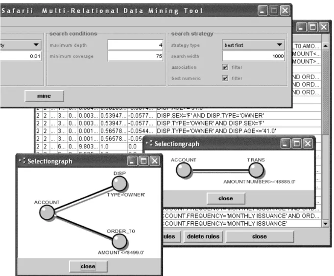
Chapter 11 considers MRDM on a more methodological level. It provides a blueprint for MRDM projects, focussing on the activities that precede the actual modelling step, and presents ProSafarii, a system that supports a user in the pre-processing phase of MRDM projects.

(16)

(17)

2 Structured Data Mining

In this chapter we give an overview of the genus of Data Mining paradigms that deal with structured data. We start with definitions of the major concepts in Structured Data Mining having to do with how structured data is represented and how knowledge can be extracted from this data. These concepts are shared by the different SDM paradigms that are the subject of the remaining sections of this chapter. We briefly outline each approach, and describe how they implement SDM. Subsequently, we describe on a more detailed level the strengths and weaknesses of each paradigm.

2.1 Structured

Data

As was outlined in Chapter 1, the central subject of analysis is the individual. We assume in Structured Data Mining that an individual consist of parts that are somehow connected to form a structured individual. Parts can be thought of as small portions of an individual that are atomic: they exhibit no internal structure. All structural relations are between parts, rather than within parts. Parts typically have a number of attributes associated with them. They can thus be thought of as tuples that behave similar to the flat individuals that are the subject of Propositional Data Mining. In general, structured individuals will not be arbitrary collections of parts. Parts will appear in a relatively small number of types, referred to as classes. All parts, over all individuals, are instances of one of the classes. A class determines which attributes are available for all instances of that class.

Definition 2.1 A class C is a triple (c, S, D) in which c is the class-name, S is the schema, a set of attributes with their domain S = {a1 : D1, …, an : Dn}, and D is the domain of C: DC =

∏

=

n

i i

D

1

.

Definition 2.2 A part of class C is a tuple (a1, …, an) ∈ DC.

(18)

18

the number of parts of a certain class that may be related to a part of some other class, and vice versa. A definition of the restrictions on relations between parts of two classes will be referred to as an association between two classes. Edges in an individual can thus be thought of as instances of an association, where the label refers to the association. It should be noted that this use of the term

association is not related to the term association rules, which indicates a popular family of models of statistical dependency [33]. The present associations are hard constraints on the data.

The central input to the Structured Data Mining process is now the database, simply a collection of individuals. Although each individual will most probably be different in parts and structure, the set of individuals will adhere to a common set of restrictions on the appearance of individuals. This collection of restrictions is referred to as the data model of the database, and consists of the definitions of available classes (including attributes) of parts, plus the definitions of associations between classes.

Example 2.1 Consider a database of molecule-descriptions. Each individual describes a molecule, and consists of parts that come in three classes: a piece of information describing general properties of the molecule (molecule), pieces of information for each atom (atom), and pieces of information for each bond between two atoms (bond). Each of these classes has a fixed set of attributes, for example atom has attributes element and charge. The parts of these three classes are related to each other through four associations: one determines which atoms belong to which molecule. Similarly there is an association that determines which bond belongs to which molecule. The two remaining associations determine the two atoms involved in each bond.

Definition 2.3 A data model is a rooted undirected connected graph M = (C, A), where: 1. C is a set of class-names

2. A ⊆C × C such that, if (c, d) ∈A, then (d, c) ∈ A.

The elements of A are called associations. The root of the graph is denoted by c0.

Definition 2.4 An individual for data model M = (C, A) is a rooted undirected connected graph i = (P, E), where P is a set of parts, and E is a set of triples (p, q, a) such that

1. a = (c, d) ∈A

2. p is a part of class c, and q is a part of class d

3. there is a unique part p0∈ P such that if (p, q, (c0, ci)) ∈E, then p = p0.

The set of all individuals for a data model M is denoted by LM.

Definition 2.5 A database for data model M is a set of individuals for M.

2.2 Search

In Chapter 1 we briefly mentioned the interesting subgroup as an important ingredient of Data Mining algorithms. A large number of subgroups will be considered by such algorithms in order to produce a manageable set of interesting subgroups that will be the basis for higher-level models of the database. Rather than being interested in subgroups as enumerations of individuals belonging to it (extensional approach), we consider short descriptions of the properties shared by all members of the subgroup (intensional approach). We refer to such descriptions as patterns. In Structured Data Mining, patterns express certain required properties concerning the presence of certain parts and structural relationships between them. Patterns can thus be used to match individuals, and define subgroups.

(19)

definition of individuals as graphs, the language will conceptually be graphical. In fact, a number of Structured Data Mining paradigms, including the Multi-Relational Data Mining approach we present in this thesis, use variations of graphs as patterns. Other paradigms, Inductive Logic Programming and Semi-Structured Data Mining, rely on existing languages for expressing structural constraints.

Definition 2.6 A pattern language is a pair Lp = (P, covers) such that P is a set of expressions, and covers is a function P × LM → {0, 1}. A pattern p ∈ P is said to cover an individual i ∈ LM iff covers(p, i) = 1. If clear from the context, we will often write Lp to denote P.

Definition 2.7 A pattern in a pattern language Lp = (P, C) is an expression p∈P.

Definition 2.8 A subgroup Sp is a set of individuals in a database D that is covered by a given pattern p: Sp = {i∈D | covers(p, i)}.

Example 2.2 Consider a database D of individuals i = (N, E), and the pattern language Lp = (P, covers), where P is the set of graphs G = (N′ , E′ ), and covers(G, i) iff there exists an injection M:

N′ → N, such that

∀e∈E′ : (M(e.p), M(e.q), a) ∈E

where a is an uninstantiated variable representing an unspecified association. This pattern language can be used to describe particular subgraphs that may or may not appear in individuals in D. The location of the root of the individuals, as well as the class and attributes of its parts are ignored. By refining P and adding more constraints on the injection M, we can define more expressive pattern languages.

Most Data Mining algorithms are characterised by an extensive search for interesting subgroups. The pattern language of choice defines a search space of patterns, which is the starting point for this search process. In order to traverse this space in a sensible, guided and efficient manner, the algorithm requires a means of judging the interestingness of a given pattern (and corresponding subgroup). In general terms we refer to such a means as a score function. Typically a score function considers the database and acquires statistics about the pattern at hand, which in turn produces a score. This score will help the algorithm to make informed decisions about the progress and direction of the search.

Most algorithms will not only use statistical information from the database to guide the search, but also a priori information about the kind of individuals that are known to exist in the database. The constraints contained in the data model concerning classes and associations tell us that we cannot expect arbitrary structures in the database. Rather, we can limit the search to patterns that are in correspondence with the data model. Restrictions on the search space based on a priori knowledge about the database, commonly referred to as declarative bias, are a very important means of keeping the search process manageable and efficient. We will consider different ways of exploiting declarative bias in Multi-Relational Data Mining throughout this thesis.

Definition 2.9 A score function is function f: Lp× 2 LM → R such that, given a database D and two patterns p and q, Sp = Sq ⇒ f(p, D) = f(q, D).

(20)

20

Because we know that the search is strongly guided by the data model of the database, we can expect a certain similarity and order in the candidate patterns to be considered. Typically, a pattern will be tested on the database by means of the score function(s), and new candidate patterns will be derived from the pattern with the obtained statistics in mind. The important step of deriving new patterns by means of minimal additions to an existing pattern is known as refinement. We will be using a refinement operator, which specifies what syntactic operations are allowed on a given pattern in order to derive more complex patterns.

The predominant search mode in Data Mining is top-down search: start with a very general pattern, and progressively consider more specific patterns. For this, we require the refinement operator to produce subgroups that are subsets of the original subgroup. We refer to a refinement operator with this additional property as a top-down refinement operator.

Definition 2.11 A pattern p is more general than a pattern q (p≥q) if all individuals covered by q

are also covered by p:

(p≥q) iff∀i : covers(q, i) → covers(p, i).

Definition 2.12 A specialisation operator is a function ρ: Lp→ 2Lp such that ∀p∈Lp: ρ(p) ⊆ {q | p

≥q}.

Definition 2.13 A refinement operator is a function ρ: Lp→ 2Lp such that, given a set of syntactic operations, ∀p∈Lp : ρ(p) = {q | q is the result of a syntactic operation on p}.

Definition 2.14 A top-down refinement operator is a refinement operator that is also a specialisation operator.

2.3 Structured Data Mining Paradigms

The basic definitions given in the previous section outline how Structured Data Mining works in general terms. The existing Structured Data Mining paradigms as introduced in Chapter 1 all exhibit these concepts in one form or another, but we will need to consider how each paradigm implements them. This will help us translate terminology and practices from one paradigm to the other. Furthermore, by viewing paradigms as instances of a generic Data Mining approach, we will be able to distinguish the properties shared by all paradigms from those that are unique to a particular paradigm. We will start with an overview of the commonalities by considering how the different paradigms implement Structured Data Mining concepts.

Graph Mining From all four Data Mining paradigms for dealing with structured data, the Graph Mining paradigm is closest in approach to our abstract definition of structured Data Mining. Individuals are simply (labelled) graphs, and the database is hence a forest of these graphs. In most approaches a node (part) is labelled, such that each part belongs to a class. Constraints on the structure of individuals in the form of a data model are typically not present. The same graphical language used to represent individuals is used as a pattern language. Graph matching is used to determine which individuals are covered by a particular pattern.

(21)

individual is rarely made explicit, although sometimes facts are grouped together, or keys are added to identify the individual. A variety of declarative bias languages is used, but they mostly share the use of mode declarations [31] in order to describe how parts can be pieced together. Mode declarations restrict how certain attributes in certain predicates may be linked by shared variables in the induced logic programs. This is a slight variation on the association concept. ILP typically uses Prolog as the pattern language. ILP algorithms often allow as input not only the database of ground facts, but also intensional predicate definitions that may help the search process for interesting patterns.

Semi-Structured Data Mining (SSDM) The most recent approach to mining in structured data, Semi-Structured Data Mining deals with a database of semi-structured text, typically represented in the popular language XML [2, 17, 32]. Although semi-structured documents contain both structural information as well as fragments of free text, most approaches focus on the structural part and treat the text fragments as discrete values without internal structure. XML documents essentially represent a rooted tree, where the tree-structure is identified by markers in the text, known as tags, and free-text appears at the nodes (and leaves) of the tree.

The existing SSDM approaches treat documents in two technically different, but effectively similar ways. One approach is to treat a single document as the database, and regard the children of the root of the semi-structured tree as individuals. The alternative approach is to take a collection of documents as the database, and treat each document as an individual. In either way, the nodes in the tree, identified by tags, correspond to the parts, and may have several attributes.

Most XML documents come with a grammar that strongly restricts the kinds of structure that are allowed in XML documents. Typically this grammar is specified in a separate file, known as a Document Type Definition (DTD) [41], which may be shared by multiple documents. Although rarely used in SSDM, DTD is ideal as a declarative bias. In the true nature of declarative bias, a DTD not only determines when XML documents are well formed, but should be used as important information to guide and prune the search process. The existing SSDM approaches boast a variety of pattern languages in order to select individuals on the basis of features of the semi-structured tree. Most algorithms employ generic graphical or tree structures that are not specific to the technology surrounding XML. A new development is to use the XPath technology [108] that has been specifically designed for applications that need to access and query specific locations within XML documents. It can be expected that XPath, or more generally XQuery [109], will play a greater role as pattern language for SSDM in the future [16].

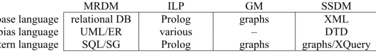
MRDM ILP GM SSDM

database language relational DB Prolog graphs XML

bias language UML/ER various – DTD

pattern language SQL/SG Prolog graphs graphs/XQuery

Table 2.1 Representation in Structured Data Mining approaches.

2.4 A

Comparison

(22)

22

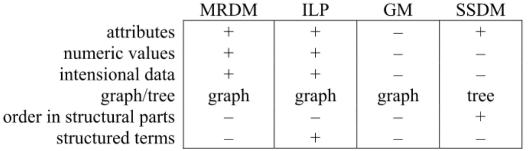
and hence on the power of the mining paradigm. Below, we give a brief comparison of some of these aspects related to the choice of representation. A summary is given in Table 2.2. It should be noted that the comparison is based on the common practices in each of the paradigms. Individual algorithms may cater to specific needs that are, however, not typical for the paradigm in question.

MRDM ILP GM SSDM

attributes + + – +

numeric values + + – –

intensional data + + – –

graph/tree graph graph graph tree

order in structural parts – – – +

structured terms – + – –

Table 2.2 Details of database representation.

Attributes ILP, SSDM and MRDM all share the notion of attributes related to parts. Attributes in all paradigms work virtually the same, although XML does not provide typing for attributes. Graph Mining is limited, as it typically does not provide for attributes at nodes in the graph. This limitation is often overcome by adding extra nodes to the graph for each attribute-value pair. This is less desirable since you loose the constraint that each attribute may have only one value.

Numeric values Attributes with numeric values typically are only treated properly in ILP and MRDM. As attributes in XML are not typed, SSDM treats numeric values as discrete values.

Intensional data Only MRDM and ILP provide for declarative definitions of (part of) the data. Intensional data is achieved in MRDM by means of view definitions: SQL queries that act as virtual tables. Intensional data is even more natural in ILP. Predicates may be defined not only by listing ground facts, but also by providing a Prolog program.

Graph/tree Only three of the SDM paradigms are able to represent individuals as full graphs. Because of its serialised nature, XML can only store tree-structured data, which restricts the power of SSDM. Admittedly, it is possible to provide links between different nodes in a tree using the ID and IDREF construct, and thus obtain more graphical structures, but this is typically not used.

Order in structural parts The textual nature of XML that causes some representational limitations also has some advantages over the other representations. Children of a parent in a tree appear in a specific order. This order may be irrelevant, which makes the parent-child relation a regular one-to-many association, but it may also be used in the analysis. Especially in sequential- or time-related domains, this may make SSDM a good choice.

(23)

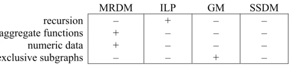
MRDM ILP GM SSDM

recursion – + – –

aggregate functions + – – –

numeric data + – – –

exclusive subgraphs – – + –

Table 2.3 Expressive power of typical SDM approaches.

Aside from the representational details in which SDM paradigms may differ, the paradigms can also be characterised by the expressive power of the pattern languages and actual algorithms used. Table 2.3 gives an overview of a number of subjects in which particular paradigms excel. Again, the classification is typical, rather than absolute.

Recursion Structured individuals may contain recursive structures: several parts of the same class may be related to each other. Recursive databases are characterised by cycles in the data model. In order to capture this cyclic dependency, a pattern language needs to support recursive definitions. As Prolog includes recursion naturally, there have been a range of ILP methods that deal with recursion. As yet, ILP is unique in this respect.

Aggregate functions So-called aggregate functions are a means of characterising groups of parts in an individual by a single value. Although they are a powerful tool for building patterns, they have received virtually no attention in ILP, GM or SSDM. Aggregate functions are covered in full detail in Chapters 4, 7, 8 and 9.

Numeric data Although both MRDM and ILP deal with numeric data, its treatment in ILP is typically very static and limited, especially in comparison with analogous algorithms in Propositional Data Mining. By relying on the computational power of the RDBMS, MRDM aims to provide the same level of support for numeric data as is customary in propositional algorithms.

Exclusive subgraphs A technical, but important difference in pattern language sets GM apart from the other paradigms. Because of the nature of graph matching involved in graphical patterns, requiring two parts to be present assumes that these two parts are distinct. This is in contrast to alternative languages such as Prolog, where multiple features can map on the same part or subgraph. The exclusive subgraph matching is convenient when the cardinality of particular parts is relevant, for example when describing hands in Poker (e.g. Full House, Pairs) or functional groups in molecules (e.g. –NH2).

This overview of the strengths and weaknesses of the four paradigms shows a number of things. First we can note that MRDM and ILP are relatively close in representational power. This comes as no surprise, as the analogy between relational databases and first-order logic is well-established. Still, the way both paradigms approach discovery is fairly different.

Compared to ILP and MRDM, GM seems to be rather poor. Important issues, such as numeric data and intensional definitions are mostly overlooked. Although its conceptual emphasis can be a fruitful source for new ideas in the analysis of structured data, it appears unlikely that GM can outperform the competing paradigms in industrial applications. One important exception is the natural treatment of exclusive subgraphs included in graph matching. This concept is as yet largely ignored in the other paradigms, but can be an essential tool in selected applications.

(24)

24

basis of XML and especially the bias language DTD are an important advantage. XML is also unique as a database language in its implicit order in parts. SSDM could be a strong candidate in domains where order is relevant, as soon as more SSDM algorithms incorporate this feature.

2.5 What’s in a Name?

There has been some debate over the appropriateness of the name Multi-Relational Data Mining. If relational databases are concerned with data in multiple tables, why use the multi-prefix for mining of such databases? As is often the case, there are historical reasons for using this name. The term

Relational Data Mining has occasionally been used in the KDD-community to describe single-table algorithms that work on data stored in relational databases. As will be clear in the remainder of this thesis Multi-Relational Data Mining is specifically concerned with the complexity stemming from having multiple tables, so the name should be clear about this.

Presently the term Relational Data Mining (as well as Relational Learning) has had some popularity among ILP researchers. This alternative name for ILP was inspired by the observation that knowledge produced by modern ILP systems can hardly be called true logic programs, and that most practical databases are of relational form rather than first-order logic. In most cases however, the Relational Data Mining label represents little more than an RDBMS-awareness. For example, the majority of contributions to the Relational Data Mining book [13] can be considered classical ILP in our definition. In our view, the two above-mentioned uses of Relational Data Mining each only satisfy one of two important hallmarks of MRDM: a focus on multiple tables, and a substantial incorporation of relational database technology.

(25)

3 Multi-Relational

Data

In the previous chapter, a general framework for mining structured data was outlined, and an overview was given of how the different Structured Data Mining paradigms approach such data. In this and the following chapter, we will describe in more detail how MRDM works, and introduce some basic concepts upon which the different MRDM techniques described in following chapters will build. We will explain how structured data is stored in a relational database, and how MRDM algorithms may query such data. A multi-relational pattern language will be introduced, along with a refinement operator that lays out a search space of multi-relational patterns for MRDM algorithms to explore.

3.1 Structured Data in Relational Form

(26)

26

three atoms and two bonds. In Figure 3.2 these parts are distributed over three tables that also contain data for other molecules, e.g. water.

Figure 3.1 CO2 and its graphical representation.

Atom

id mol_id element

Molecule 1 1 C Bond

id name 2 1 O id atom1 atom2 type

1 CO2 3 1 O 1 1 2 double

2 H2O 4 2 H 2 1 3 double

5 2 H 3 4 6 single

6 2 O 4 5 6 single

Figure 3.2 Relational representation of CO2 and H2O.

3.2 Multi-Relational Data Models

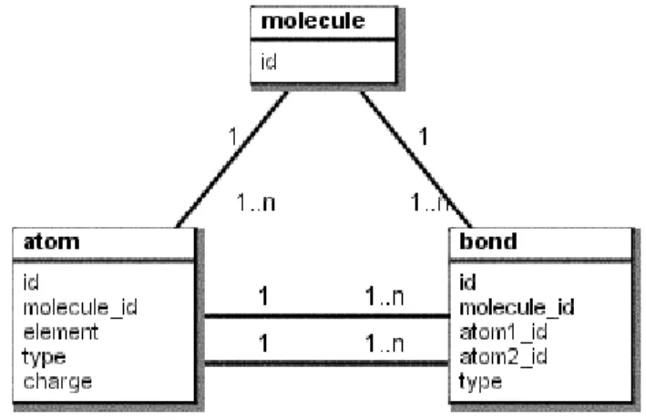
An important piece of information in Multi-Relational Data Mining is the data model of the database [61]. It contains a description of the structure of the database in terms of the tables and relationships between them. It provides a list of schemata of the tables: specifications of the available attributes (e.g. numeric, nominal). Furthermore, it provides information about associations between tables: specifications of how records in one table relate to records in another table. Associations can be seen as slight generalisations of the foreign key notion. They specify that two tables are related, and determine a number of details concerning the relationship, but do not fix the actual implementation of this. In practice however, an association in a relational database will always appear as a primary key-foreign key pair along with the necessary referential integrity constraint.

Associations are a bit more specific than foreign key constraints. They determine in greater detail the cardinality of the relationship between two tables, something which we will refer to as the

multiplicity of the association. For example, we may specify that any record in one table relates to multiple, but at least one, records in another table. Such information may be very valuable to guide the Data Mining process but of less use to the integrity of the database, hence the difference between associations and foreign key constraints. Associations provide multiplicities in two directions, one for each table involved. Typically, we will be using the following four values per multiplicity:

Atom

Atom Molecule

Bond

Bond el = C

el = O

type = double

type = double O = C = O

(27)

• Zero or one (0..1)

• One (1)

• Zero or more (0..n)

• One or more (1..n)

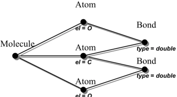
As was proposed in [61], a visual modelling language for specifying the data model will be used, namely the Class Diagrams that are part of the Unified Modeling Language (UML) [92, 94]. This language was developed for modelling databases (as well as object oriented systems) and contains a subset of visual elements that exactly fit our needs. Figure 3.3 shows a UML Class Diagram for our molecular example.

As can be seen, there are three classes: molecule, atom and bond. Four associations between these classes determine how objects in each class relate to objects in another class. As a bond involves 2 atoms (in different roles) there are two associations between atom and bond. The multiplicity of an association determines how many objects in one class correspond to a single object in another class. For example, a molecule has one or more atoms, but an atom belongs to exactly one molecule.

Figure 3.3 UML Class Diagram of a molecular database.

Why do we wish to use UML to express bias? First of all, as UML is an intuitive visual language, essentially consisting of annotated graphs, it is easy to write down the declarative bias for a particular domain or judge the complexity of a given data model. Another reason for using UML is its widespread use in database modelling. UML has effectively become a standard with thorough support in many commercial tools. Some tools allow the reverse engineering of a data model from a given relational database, directly using the table specifications and foreign key relations.

(28)

28

<?xml version="1.0"?>

<!DOCTYPE mrml SYSTEM "mrml.dtd"> <mrml>

…

<name>molecule001</name> <table>

</attribute>

<attribute id="ATOMID2" type="key"> <name>molecule_id</name>

</attribute>

<attribute type="nominal"> <name>element</name> </attribute>

</table> <table>

… </table>

<association direction="forward"> <name>molecule atom</name>

<association direction="forward"> …

</association> </datamodel>

</mrml>

3.3 Structure of the Data Model

Although the information contained in the data model is generally sufficient for defining the search space of patterns considered by MRDM (or even SDM) algorithms, it often pays off to examine the structure of the data model in more detail. This examination will yield a better insight into how the search will proceed, and what results can be expected. It will also support important choices on a more procedural level, such as the definition of training and test set. Furthermore, the data model may be related to what a domain expert will know of the nature of structures present in the database. This may lead to further sources of declarative bias that are impossible to express in MRML.

3.3.1 Tables and their Roles

(29)

• Foreground-data The foreground typically consists of tables that describe the primary domain that will be analysed. The data is gathered in-house, and is of a dynamic nature, often a snapshot of an operational system.

• Background-data The background, on the other hand, consists of tables that describe static knowledge about the outside world (demographics, periodic table of elements, etc.) that is not specific to the problem domain, and often of aggregated nature. It is thus the complement of the foreground.

• Individual-data Tables belonging to this set contain data that is individual-specific: the records in the target table define disjoint sets of records in the tables of individual-data. If a record in a table belongs to two individuals, then this table is not part of the individual-data. In order to determine whether a table belongs to the individual-data, we will have to determine the multiplicity of any of the transitive associations between this table and the target table. If this transitive association is one-to-many or many-to-many, a single record may belong to multiple individuals, and the table is not part of the individual-data.

The previously defined sets of tables influence the analysis in later stages. Let us consider the relation between foreground and individual-data. If these two sets coincide, there is a clear boundary of individuals in the data model. No dynamic data from the foreground is shared between individuals. This situation is known as the learning from interpretations setting in ILP [13, 31], and has a number of advantages. The most important of these is that sampling is straightforward: any division in the target table will divide the data in non-overlapping sets. This is important in later stages for internal validation, separation between training and test sets, and scalable implementations [13].

In the case where the individual-data is a proper subset of the foreground, the boundaries between individuals are unclear, and part of the data is shared. Any sampling will have to be done with greater care in order to prevent a bias on processes using samples, for example cross-validation. If the overlap has too great an influence, any tables that are part of the foreground, but not of individual-data should be left out.

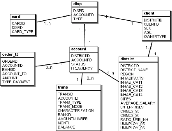
Example 3.1 Figure 3.4 shows the Financial database, taken from the Discovery Challenge organised at PKDD ’99 and PKDD 2000 [106]. The database is based on data from a Czech bank. It describes the operations of 5369 clients holding 4500 accounts. The data is stored in seven tables, three of which describe the activities of clients. Three further tables describe client and account information, and the remaining table contains demographic information about 77 Czech districts. We have chosen the account table as our target table.

The background of the Financial dataset consists of a single table: district. All other tables contain dynamic data that is gathered specifically for the financial domain, and thus belong to the foreground. Given the selected target table account, the individual-data consists of all tables except the two tables district and client. Clearly district-information is shared between many individuals (accounts). Although not directly clear from the data model, we can deduce from the existence of disp that there is a many-to-many relationship between accounts and clients. Therefore, clients may have multiple accounts, which excludes client from the individual-data.

(30)

30

Figure 3.4 The Financial database.

It should be noted that intensional tables (views) do not necessarily belong to the background. Although the definition of these tables is often based on common, static knowledge about the world, the actual data represented by the intensional table can just as well be foreground. This is because it can be derived from the dynamic data in foreground tables, and can be considered a reformulation of this data.

Note also that alternative definitions of the background (and hence the foreground) have been used, particularly in the ILP field. The following uses have appeared in the literature:

• The background consists of every table (extensional or intensional) other than the target table.

• The background consists of every table that is not individual-specific (foreground equals individual-data). In the learning from interpretations setting this coincides with our own definition.

• The background consists of all intensionally defined tables (i.e. views or predicate definitions).

3.3.2 Directions

In general Multi-Relational Data Mining algorithms will traverse the graph of tables and associations, which makes the data model a strong way of guiding the search process. In many cases however, the data model is too general and not all paths are desirable. Data models may contain redundant associations that are useful for describing structural information in alternative ways, but harm the search process if the redundancy is not made explicit.

(31)

associated with another molecule than the molecule its two atoms belong to, the data model does not exclude this. Therefore, the data model suggests patterns that are known to be impossible, and MDRM algorithms will waste time considering these patterns. The alternative paths in a data model should be explored during the search, but never together in the same pattern.

Directed associations are a good way to specify this extra declarative bias, as well as to further control the produced results. If an association between two tables is directed, the search process can only introduce information in one table after the other table is introduced, in the direction of the association and not vice-versa. Directions can best be added in the following cases:

• redundant associations. An association is redundant if it represents a relation between two tables that is also represented by several other associations combined. The redundancy in Example 3.2 is solved by adding directions away from molecule.

(32)

(33)

4 Multi-Relational

Patterns

4.1 Local

Structure

It has become clear that individuals, and even more importantly groups of individuals, are the main subject of analysis in MRDM. Now that we know how individuals are represented in relational databases, we should consider how to query databases of individuals, and select subgroups that share certain structural characteristics. In our MRDM framework we will mainly express such structural characteristics by building on conditions at the low level of relationships between pairs of tables. For example we will select candidate subgroups of molecules by extracting structural features from the molecule and the atom table and the association between them. We will refer to such incomplete and localised information as local structure. By combining conditions on the local structure (not necessarily involving the target table) we end up with expressions about individuals. Local structure involves data in two tables, but more importantly, the association between them. The association will typically be one-to-many (or many-to-one depending on the order of the two tables). Such a one-to-many relationship basically defines a grouping on the records in the table on the ‘many’ side, as demonstrated below:

We can select records in one table on the basis of features of the associated group of records in the other table. This way of extracting information about local structure by means of describing groups of records will be the primary approach to building descriptions of individuals.

(34)

34

applicable algorithms. In this thesis, we dedicate a number of chapters to each approach. These approaches are:

• Conditions on the occurrence within the group of records with a particular characteristic. These so-called existential features typically involve one or more attributes of the records, but can also just refer to the existence of a record, or of records that are again related to records in the other tables through other associations. This approach has been the predominant mode of work in other Structured Data Mining frameworks, such as Inductive Logic Programming and Graph Mining. In this introductory chapter and the following two chapters, we will limit the discussion to this approach.

• Conditions on the group of records as a whole. By means of so-called aggregate functions

we can describe a group in a variety of ways. For example, groups can be selected on the basis of their size or on the average value within the group of a particular numeric attribute. Such conditions are a superset of the existential conditions, as we can include the exists

aggregate function. The approach based on aggregate functions has only recently been receiving attention in the field of Structured Data Mining [38, 59, 63, 68, 69, 84, 85]. Chapters 7 through 9 cover the possibilities and limitations of aggregate functions.

4.2 Pattern

language

If we want to select subgroups of individuals on the basis of structural properties they possess, we need to define a language that is capable of expressing existential conditions. We will be using the

selection graph language to express multi-relational patterns:

Definition 4.1: A selection graph G is a pair (N, E), where N is a set of pairs (t, C) called selection nodes, t is a table in the data model and C is a, possibly empty, set of conditions on attributes in t of type (t.a θ c).θ is one of the following operators, =, ≤ , ≥.

E is a set of triples (p, q, a) called selection edges, where p and q are selection nodes and a is an association between p.t and q.t in the data model. The selection graph contains at least one node n0

that corresponds to the target table t0.

Definition 4.2 An empty selection graph is a selection graph that contains no edges or conditions: ({(t0, ∅)}, ∅).

Definition 4.3 Let i = (P, E) be an individual and G = (N, E′) be a selection graph. G covers i

(covers(G, i)) iff there exists a function M: N→ P such that 1. M(n0) = p0

2. ∀n∈N: M(n) satisfies the set of conditions n.C

3. ∀e∈E′ : (M(e.p), M(e.q), e.a) ∈E

Note that although the covers relation is concerned with the occurrence of particular graphical structures in individuals, it is not the same as the graph matching employed in Graph Mining. For selection graphs to act as subgraphs of individuals, we would have to add the extra constraint that the function M is an injection: n≠n′ implies M(n) ≠M(n′ ).

Definition 4.4 The selection graph language SG is a pattern language SG = (P, covers), where P is the set of possible selection graphs.

(35)

records in the corresponding table n.t that is determined by the set of conditions n.C and the relationship with records in other tables characterised by selection edges connected to n. Selection graphs are more intuitive than expressions in SQL or Prolog, because they reflect the structure of the data model, and refinements to existing graphs may be defined in terms of additions of edges and nodes.

A selection graph can be translated into SQL or Prolog in a straightforward manner. The following algorithm shows the translation into SQL. It will produce a list of tables table_list, a list of join conditions join_list, and a list of conditions condition_list, and combine these to produce a SQL-statement. A similar translation to Prolog can be made.

TranslateSelectionGraph(selection graph G)

table_list = '' condition_list = '' join_list = ''

for each node i in G.N do

table_list.add(i.table_name + ' T' + i) for each condition c in i do

condition_list.add('T' + i + '.' + c) for each edge e in G.E do

join_list.add(e.left_node + '.' + e.left_attribute + ' = ' + e.right_node + '.' + e.right_attribute) return 'SELECT DISTINCT T0. ' + t0.primary_key +

' FROM ' + table_list + ' WHERE ' + join_list + ' AND ' + condition_list

Example 4.1 The following selection graph, and its corresponding SQL statement, represents the set of molecules that have a bond, and a C-atom.

SELECT DISTINCT T0.id

FROM molecule T0, bond T1, atom T2

WHERE T0.id = T1.molecule_id and T0.id = T2.molecule_id AND T2.element = 'C'

4.2.1 Refinements

The selection graph language provides a search space of multi-relational patterns for MRDM algorithms to explore. The MRDM algorithms in this thesis all traverse this search space in a top-down fashion: starting with a simple, very general pattern, progressively consider more complex and specific selection graphs. A refinement operator defines in more detail how this top-down traversal works.

Atom Molecule

Bond