sim.7351.pdf

Modeling

event

count

data

in

the

presence

of

informative

dropout

with

application

to

bleeding

and

transfusion

events

in

myelodysplastic

syndrome

Guoqing

Diao,

Donglin

Zeng,

Kuolung

Hu

and

Joseph

G.

Ibrahim

Inmanybiomedicalstudies,itisoftenofinteresttomodeleventcountdataoverthestudyperiod.Forsome patients,wemaynotfollowupthemfortheentirestudyperiodowingtoinformativedropout.Thedropouttime canpotentiallyprovidevaluableinsightontherateoftheevents.Weproposeajointsemiparametricmodelfor eventcountdataandinformativedropouttimethatallowsforcorrelationthroughaGammafrailty.Wedevelop efficientl ikelihood-basede stimationa ndi nferencep rocedures.T hep roposedn onparametricm aximum likeli-hoodestimatorsareshowntobeconsistentandasymptoticallynormal.Furthermore,theasymptoticcovariances ofthefinite-dimensionalparameterestimatesattainthesemiparametricefficiencybound.Extensivesimulation studiesdemonstratethat theproposed methodsperform well in practice.Weillustratethe proposed meth-odsthroughanapplicationtoaclinicaltrialforbleedingandtransfusioneventsinmyelodysplasticsyndrome. Copyright©2017JohnWiley&Sons,Ltd.

Keywords: Coxmodel;informativedropout;nonparametricmaximumlikelihoodestimators;Poissonregression model; semiparametric efficiency

1. Introduction

Recurrent events data refer to a subject experiencing repeated occurrences of the same or related types of events during the study time. The number of the event count during the time is clearly the interest in medical and epidemiological researches. Many clinical trials are designed to demonstrate treatment efficacy or safety based on the frequency of the events over time, defined as the event rate. Although the exposure period may be different from subject to subject, the frequency of events is usually summarized as a rate or number per year or per 100 subject years of exposure. Examples include occurrence of serious infections in clinical trials of AIDS prophylaxis [1], relapses of multiple sclerosis [2], the frequency of secondary infections during myelosuppressive chemotherapy treatment [3], or the occurrence of red blood transfusions [4].

The Poisson regression model is straightforward in analyzing this type of data, and it has been illus-trated in many papers; for instance, see [5–9]. Typically, the event count data are assumed to follow a Poisson distribution conditional on the follow-up time, and the logarithm of the follow-up time is treated as a fixed intercept in the Poisson regression model. However, the number of events can potentially impact the dropout time, and additional information on the informative dropout time can provide more insight in the estimation and inference of the Poisson rates. It is therefore very important to account for potential correlation between the event count data and informative dropout time.

a_{Department of Statistics, George Mason University, Fairfax, VA, U.S.A.}

b_{Department of Biostatistics, University of North Carolina at Chapel Hill, Chapel Hill, NC, U.S.A.}

c_{Amgen Inc., One Amgen Center Drive, Thousand Oaks, CA, U.S.A.}

*Correspondence to: Guoqing Diao, Department of Statistics, George Mason University, Fairfax, VA 22030, U.S.A.

A motivating example involves a phase 2, multicenter, randomized, double-blind, placebo-controlled clinical trial with low or intermediate-1 risk myelodysplastic syndrome (MDS) patients that have severe thrombocytopenia (platelet counts<50×109/L). The key study objective is to evaluate the treatment effect on reduction of both platelet transfusion incidences and bleeding adverse events reported during the study efficacy follow-up (duration of 26 weeks). Living with abnormal platelet function, severe throm-bocytopenia patients have an increased risk of bleeding incidence. Platelet transfusion interventions are often required therapeutically (given to patients who are actively bleeding) and prophylactically (to pre-vent future bleeding). Therefore, the incidence of platelet transfusion interpre-vention and bleeding epre-vent occurrence are highly correlated. In addition, thrombocytopenia in the MDS population is associated with shortened survival and an increased risk of evolution to acute myeloid leukemia, part of the natural progression of MDS. During this period, patients may obtain disease progression and then discontinue the treatment and dropout of the study in order to receive the MDS disease-modifying treatment. There were also patients that were informatively censored owing to death or administrative withdrawal due to other types of adverse events.

Several authors have proposed nonparametric or semiparametric methods to jointly model recurrent event data and informative follow-up time. In particular, Wanget al. [10] and Huang and Wang [11] model the association between the intensity of the recurrent event process and the hazard of the fail-ure time through a common subject-specific latent variable. They propose a ‘borrow-strength estimation procedure’ by first estimating the value of the latent variable from the recurrent event data and then use the estimated value in the failure time model. Alternatively, several authors have proposed to use frailty models to account for the correlation between the recurrent event process and terminal event process [12–17]. In these papers, the recurrent event times are assumed to be observed before the dropout time. A comprehensive review of statistical analysis of recurrent event data was provided in [18].

In many applications, we do not observe the event times directly. Instead, only the number of recurrent events during the follow-up period is available. Such data are often referred to as the panel count data. For correlated panel count data, Zhang and Jamshidian [19] and Yaoet al.[20] proposed Gamma frailty Poisson models but assumed conditional independent observation processes. Among others, several stud-ies [21–27] proposed semiparametric regression analysis of panel count data with dependent observation processes. Essentially all of these existing methods are based on estimating equations, and it is not clear whether the estimators are asymptotically efficient. Additionally the bootstrap method is often needed to estimate the standard errors of the parameter estimates. Furthermore, these papers focus on parameter estimation, and little has been investigated in comparing the event rates of two treatment groups. Sun and Zhao [28] gave a thorough review of the statistical analysis of panel count data.

In this paper, we develop likelihood-based methods to compare the event rates in the treatment group and placebo group adjusting for covariates and meanwhile accounting for informative dropout. In Section 2, we propose a joint model of the event count data and hazard of the dropout time and allow for correlation by using a Gamma frailty. Unlike most existing joint models (e.g., [21, 23, 24]), we model the cumulative mean count at each time instead of assuming a Poisson process for the recurrent data and modeling the whole intensity function. To achieve more flexibility and robustness, we consider a stratified Cox model for the informative dropout time, allowing for unspecified (conditional) baseline hazard in each treatment group. We derive the nonparametric likelihood function of the unknown param-eters based on the observed data. In addition, we describe several tests for comparing the incidence rates between the treatment group and the placebo group. In Section 3, we establish the asymptotic proper-ties of the proposed nonparametric maximum likelihood estimators (NPMLEs). The proposed NPMLEs are shown to be consistent and asymptotically normal. Furthermore, the asymptotic covariances of the finite-dimensional parameter estimates attain the semiparametric efficiency bound. Extensive simulation results are provided in Section 4. We illustrate the proposed methodology through the MDS clinical trial in Section 5. We conclude the paper with a few brief remarks in Section 6. All technical details of the proofs of the asymptotic results are relegated to the Appendix.

2. Methods

pointt; and𝐙iis ad×1 vector of covariates at baseline. Therefore, the observed data are {

A_i,𝐙i,X_i=N_i(T_i),T_i≡T̃_i∧C_i,Δ_i=I(T̃_i⩽C_i) }

, i=1,…,n,

where theT_i’s are the observed follow-up times, andΔ_iare the corresponding censoring indicators. Denote the end of study by 𝜏. For subject i, we assume that N_i(t),t ∈ [0, 𝜏] follows a Poisson distribution with

E{N_i(t)|𝜉_i,A_i,𝐙i} =𝜆_A

i𝜉itexp(𝜷

T_{𝐙i), (1)}

where𝜆_A

iis the conditional baseline event rate in groupAi,𝜉i∼Gamma(𝜃

−1_{, 𝜃}−1_{)represents the patient’s} heterogeneity due to other characteristics, and𝜷is a set of regression coefficients. The gamma frailties 𝜉ihave mean 1 and variance𝜃and are mutually independent. It is worth to note that unconditional on𝜉i,

the rate function satisfiesE{N_i(t)∕t|A_i,𝐙i} =𝜆_A

iexp(𝜷 T_𝐙i).

While model (1) is a parametric model, we assume a semiparametric model for the informative dropout time. Specifically, we further assume thatT̃_iis independent ofN_i(t)given𝜉_iand the conditional hazard function ofT̃_iis

h(t|𝜉_i,A_i,𝐙i) =𝜉_ih_A

i(t)exp(𝜻

T_{𝐙i), t∈ [0, 𝜏], (2)}

where𝜉_ih_A

i(t)is the conditional baseline hazard function ofT̃igiven𝜉iand𝐙i, and𝜻is a set of regression

coefficients. The functionsh₀(t)andh₁(t)are unspecified. Model (2) is referred to as the Cox model with a shared Gamma frailty [29, 30]. This model allows one to model the positive correlation between the event rate of the Poisson process and the hazard rate of the time to adverse event or death. Additionally, model (2) is also a stratified model allowing the (conditional) baseline hazards to be different in the control and treatment groups. Note that we may allow different covariates in models (1) and (2).

WriteH_a(t) =∫₀th_a(s)ds,a=0,1. From model (2), we can show by using the Bayes rule that condi-tional on{A_i,𝐙i,T_i,Δ_i}, the distribution of𝜉_iisΓ(𝜃−1_{+ Δ}

i, 𝜃−1+HAi(Ti)e

𝜻T_𝐙

i_{). Then we can show that}

conditional on{A_i,𝐙i,T_i,Δ_i}, the distribution ofX_iis negative binomial with parameters𝜃−1_{+ Δ}

iand

success probability

𝜆AiTie

𝜷T_𝐙 i

𝜃−1_+H

Ai(Ti)e

𝜻T_𝐙 i+𝜆

AiTie

𝜷T_𝐙 i

.

The conditional mean and variance ofX_igiven{A_i,𝐙i,T_i,Δ_i}are given by

(𝜃−1+ Δ_i) 𝜆AiTie

𝜷T_𝐙 i

𝜃−1_+H

Ai(Ti)e𝜻 T_𝐙

i

, (3)

and

(𝜃−1+H_A

i(Ti)e

𝜻T_𝐙 i₊𝜆

AiTie

𝜷T_𝐙

i₎₍𝜃−1_{+ Δ} i)

𝜆AiTie

𝜷T_𝐙 i

(𝜃−1_+H

Ai(Ti)e

𝜻T_𝐙 i)2

, (4)

respectively. Therefore, by introducing a Gamma frailty, we allow for overdispersion in the recurrent events data. Furthermore, the Gamma frailty allows for correlation between the recurrent events and the follow-up time, and consequently, the distribution ofX_idepends on the parameters not only in the Poisson model (1) but also in the survival model (2).

Write𝝓= (𝜆₀, 𝜆₁, 𝜃,𝜷,𝜻). Assume that, conditional onAand𝐙, the censoring timeCis independent of the failure timeT̃ and the event countX. Based on the observed data, the likelihood function for the unknown parameters(𝝓,H₀,H₁)is

L(𝝓,H₀,H₁) =

n

∏

i=1 ∫𝜉i

(𝜆_A

i𝜉iTie

𝜷T_𝐙

i)Xiexp{−𝜆 Ai𝜉iTie

𝜷T_𝐙 i}

X_i!

× {h_A

i(Ti)𝜉ie

𝜻T_𝐙

i_}Δi_exp{−H Ai(Ti)𝜉ie

𝜻T_𝐙 i_}f(𝜉

i)d𝜉i,

wheref(⋅)is theGamma(𝜃−1_{, 𝜃}−1_{)density given by}

f(𝜉) = 𝜃

−𝜃−1

Γ(𝜃−1₎𝜉 𝜃−1₋₁

e−𝜉∕𝜃.

The likelihood (5) is equivalent to

L(𝝓,H₀,H₁) =

n

∏

i=1

TXi i

X_i! (

𝜆Aie

𝜷T_𝐙 i

)Xi{

h_A

i(Ti)e

𝜻T_𝐙 i

}Δi Γ(𝜃−1+X_i+ Δ_i)

Γ(𝜃−1₎

× 𝜃

Xi+Δi

[

1+𝜃{𝜆_A

iTie

𝜷T_𝐙 i+H

Ai(Ti)e

𝜻T_𝐙 i}]𝜃

−1_+X

i+Δi.

We propose to estimateH_a(⋅),a =0,1 nonparametrically by leaving both functions unspecified. By using the nonparametric maximum likelihood approach and allowingH_a(⋅),a = 0,1 to be right con-tinuous, we obtain the nonparametric likelihood function, still denoted by L(𝝓,H₀,H₁), for ease of exposition,

L(𝝓,H₀,H₁) =

n

∏

i=1

TXi i

X_i! (

𝜆Aie

𝜷T_𝐙 i

)Xi(

H_A

i{Ti}e

𝜻T_𝐙 i

)Δi Γ(𝜃−1+X_i+ Δ_i)

Γ(𝜃−1₎

× 𝜃

Xi+Δi

[

1+𝜃{𝜆_A

iTie

𝜷T_𝐙

i +H

Ai(Ti)e

𝜻T_𝐙 i}]𝜃

−1_+X

i+Δi,

whereH_a{t},a =0,1, is the jump size ofH_a(⋅)att. After some simple algebra, we can show that the log-likelihood function of(𝝓,H₀,H₁)is given by

l(𝝓,H₀,H₁) =c+

n

∑

i=1 [

X_i(log𝜆_Ai+𝜷T𝐙i) + Δ_i[logH_Ai{T_i} +𝜻T𝐙i] +

Xi+Δ∑i−1

k=0

log(𝜃−1+k)

+ (X_i+ Δ_i)log𝜃− (𝜃−1+X_i+ Δ_i)log{1+𝜃𝜆_AiT_ie𝜷T𝐙i₊𝜃_H

Ai(Ti)e𝜻 T_𝐙

i_}

] ,

wherecis a constant. We maximizel(𝝓,H₀,H₁) and obtain the NPMLEs of (𝝓,H₀,H₁), denoted by (𝝓̂_n, ̂H_0n, ̂H_1n). The maximization can be accomplished by using an iterative procedure such as the quasi-Newton algorithm Presset al.[31]. The quasi-Newton algorithm has been successfully applied in optimization problems with a large number of parameters [32, 33] and has been implemented in software packages such as sas, r, and matlab. Section 3 establishes the consistency and asymptotic normality of the NPMLEs.

Note that our main interest is to test𝜆₀=𝜆₁. We consider several different tests: (i) likelihood ratio test; (ii) Wald test based on ̂𝜆₀−̂𝜆₁; (iii) Wald test based on ̂𝜆₀∕̂𝜆₁; and (iv) Wald test based on log ̂𝜆₀−loĝ𝜆₁. It can be shown from the asymptotic results in Section 3 that under the null hypothesis, all four test statistics are asymptotically chi-square with 1 degree of freedom.

Remark 2.1

When the follow-up time is short, we can assumeh₀(t) =h₀andh₁(t) =h₁. Furthermore, if we assume that there are no covariates effects and reparameterize

p_a =𝜆_a∕(𝜆_a+h_a), 𝜈_a =𝜃(𝜆_a+h_a),

fora=0,1, then the likelihood function for the unknown parameters𝝓≡(p₀, 𝜈₀,p₁, 𝜈₁, 𝜃)takes the form

L(𝝓) =

n

∏

i=1 (

X_i+ Δ_i

X_i

)

pXi

Ai(1−pAi) ΔiΓ(𝜃

−1_+X

i+ Δi)

(X_i+ Δ_i)!Γ(𝜃−1₎ (𝜈_A

iTi) Xi+Δi

[ 1+𝜈_A

iTi

]𝜃−1_+X

Concerning the inference for the parameters, we can assume that theT’s are fixed and that the data are generated from the following mechanism: in armA=0, conditional onT_i,X_i+Δ_ifollows a negative bino-mial distributionNB(𝜃−1_{, 𝜈}

0Ti∕(1+𝜈0Ti))and conditional onXi+ Δi,Xifollows a binomial distribution,

Binomial(X_i+ Δ_i,p₀). This also holds forA=1.

3. Asymptotic results

In this section, we establish the asymptotic properties of the proposed NPMLEs. In particular, we will prove the following three theorems.

Theorem 1

Under the conditional independent censoring assumption and conditions (C1)–(C4) in Appendix A, the unknown parameters(𝝓,H₀,H₁)are identifiable.

The proof of Theorem 1 is given in Appendix B.

Theorem 2

Under the conditional independent censoring assumption and conditions (C1)–(C4) in Appendix A, with probability tending to 1,

||𝝓̂n−𝝓0||+ sup

t∈[0,𝜏a]

|Ĥ_0n(t) −H₀₀(t)|+ sup

t∈[0,𝜏a]

|Ĥ_1n(t) −H₀₁(t)|→0,

where||⋅||is the Euclidean norm.

Remark 3.1

Theorem 2 states the consistency of the NPMLEs. The basic idea for proving Theorem 2 is as follows. We first show that neitherĤ_0n(𝜏)norĤ_1n(𝜏)is allowed to diverge by using the partitioning argument described in [29]. Once the boundedness ofĤ_0n(𝜏)andĤ_1n(𝜏)is established, a subsequence ofĤ_an,a=0,1 can be found to converge pointwise to a bounded monotone functionH∗

a in[0, 𝜏]and the same subsequence of

̂

𝝓nto some𝝓∗. We construct a step functionH̄anwith jumps at the observed failure times converging to

H_a0. Then, asl_n(𝝓̂_n, ̂H_0n, ̂H_1n)⩾l_n(𝝓₀, ̄H₀n, ̄H_1n), by taking the limit, we prove that the Kullback–Leibler information between the true density and the density indexed by(𝝓∗,H∗

0,H

∗

1)is non-positive. Therefore, the true density must be equal to the density indexed by(𝝓∗,H∗

0,H

∗

1). Consistency will then follow from the identifiability result. The details of the proofs are given in Appendix C.

Theorem 3

Under the conditional independent censoring assumption and conditions (C1)–(C4) in Appendix A,

n1∕2(𝝓̂_n−𝝓₀, ̂H_0n−H₀₀, ̂H_1n−H₀₁)→_d G,

whereGis a continuous zero-mean Gaussian process in the metric spacel∞_(H)and

H={(𝐡₁,h₂,h₃) ∶𝐡₁ ∈R3+2d,h₂andh₃are functions on[0, 𝜏]; ||h1||⩽1,|h2|_V⩽1,|h3|_V⩽1}.

Here|h|_Vdenotes the total variation ofhin[0, 𝜏]andl∞_{(H)is the collection of all bounded functions on}

H. Additionally,𝝓̂_nis asymptotically efficient.

Remark 3.2

In the statement of Theorem 3, asymptotically efficient estimators mean that the asymptotic covariances attain the semiparametric efficiency bound [34, Chapter 3]. Once the consistency of the NPMLEs is established, the asymptotic distribution of the NPMLEs stated in Theorem 3 can be derived by verifying the four conditions in Theorem 3.3.1 of [35]. The proof of Theorem 3 is given in Appendix D.

Remark 3.3

Theorem 3 implies that for any (𝐡₁,h₂,h₃) ∈ H, √n(𝝓̂_n −𝝓₀)T_𝐡

1 + √

n∫₀𝜏h₂(t)d(Ĥ_0n −H₀₀) + √

observed failure times as parameters. Following the arguments in Theorem 2 of [36], we can then esti-mate the asymptotic covariance matrix of the unknown parameters by inverting the observed information matrix according to parametric likelihood theory.

Remark 3.4

Using the arguments in [37], we can prove that under the conditional independent censoring assumption and conditions (C1)–(C4) in Appendix A, the asymptotic null distribution of the likelihood ratio test statistic for testing𝜃 =0 is a 50:50 mixture of𝜒2

0 and𝜒 2 1.

4. Simulation studies

We conduct extensive simulation studies to evaluate the finite-sample performance of the MLEs of𝝓 under the proposed model. We generate data under the proposed joint model and set the true parameters

as(𝜆₀, 𝜆₁) = (1,1). We generate the follow-up time from a Weibull distribution with H_a(t) = 0.5tb

and varybamong(0.7,1.0,1.3). The variance of the Gamma frailty varies from 0.5 to 1. We generate 100 subjects for each treatment group, that is,n₀ = n₁ = 100. We use the quasi-Newton algorithm to maximize the nonparametric maximum likelihood function. The covariance matrix of the NPMLEs is estimated by inverting the observed Fisher information matrix, that is, the negative second derivatives of the nonparametric log-likelihood with respect to the finite-dimensional parameters and the jump sizes ofH₀(⋅)andH₁(⋅)at the observed dropout times. The quasi-Newton algorithm converges quickly and is robust to the choices of the initial values of the unknown parameters. It takes about 0.01 s to analyze one simulated data set (including covariance matrix estimation) under the aforementioned simulation setting on a MacBook Pro with 2.8-GHz Intel Core i7 processors.

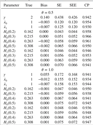
Tables I presents the summary statistics of the NPMLEs of the unknown parameters based on 1000 replicates forb=0.7. Throughout this section,𝛾≡𝜃−1_{. The proposed NPMLEs have small biases, the} estimated standard errors reflect the actual variation of the estimators, and the coverage probabilities of the

Table I.Summary statistics of the NPMLEs withn0= n₁=100 andH_a(t) =0.5t0.7_.

Parameter True Bias SE SEE CP

𝜃=0.5

𝛾 2 0.140 0.438 0.426 0.942

𝜆0 1 −0.003 0.120 0.120 0.954

𝜆1 1 −0.007 0.125 0.120 0.930

H₀(0.2) 0.162 0.000 0.043 0.044 0.958

H0(0.3) 0.215 0.000 0.051 0.052 0.966

H₀(0.4) 0.263 −0.002 0.058 0.059 0.961

H0(0.5) 0.308 −0.002 0.065 0.066 0.950

H₁(0.2) 0.162 0.001 0.046 0.044 0.946

H1(0.3) 0.215 0.001 0.056 0.052 0.953

H1(0.4) 0.263 0.000 0.063 0.059 0.950

H₁(0.5) 0.308 0.000 0.070 0.066 0.941

𝜃=1.0

𝛾 1 0.055 0.172 0.168 0.941

𝜆0 1 −0.012 0.155 0.152 0.934

𝜆1 1 −0.007 0.158 0.153 0.944

H0(0.2) 0.162 −0.001 0.047 0.046 0.950

H₀(0.3) 0.215 −0.001 0.059 0.056 0.938

H₀(0.4) 0.263 0.000 0.067 0.064 0.941

H0(0.5) 0.308 0.000 0.075 0.072 0.945

H₁(0.2) 0.162 0.001 0.048 0.046 0.936

H1(0.3) 0.215 0.001 0.059 0.056 0.948

H₁(0.4) 0.263 0.000 0.068 0.064 0.945

H1(0.5) 0.308 0.001 0.075 0.072 0.947

95% confidence intervals are close to the nominal level. Results for the scenarios whenb=1 andb=1.3 are presented in Tables S1 and S2, and similar results are obtained. We conducted additional simulations by increasing the sample size from 100 to 200 in each treatment group. The results are summarized in Tables S3–S5. Biases and standard errors of the NPMLEs, and the coverage probabilities of the 95% confidence intervals improve as sample size increases. The standard errors decrease by a factor of√2 suggesting root-nconvergence rate of the NPMLEs.

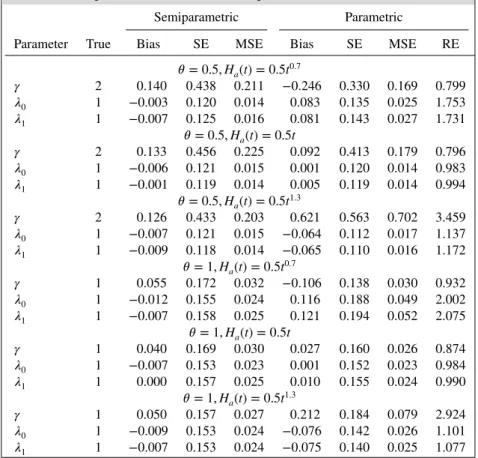
For comparison, we also consider the parametric method described in Section 2 in whichH_a(t),a= 0,1 are assumed to be constant. Table II presents the results based on 1000 replicates withn₀ =n₁ = 100 comparing the performance of the NPMLEs and the parametric MLEs. The NPMLEs are robust to departures from the parametric assumption on the baseline hazards and has little loss of efficiency compared with the parametric MLEs when the parametric assumption is true (i.e., whenb = 1). On the other hand, the parametric method tends to have biased estimators under model mis-specification especially for the case ofb=1.3. Whenb=0.7, the parametric MLEs of𝜆₀and𝜆₁have larger standard errors than the NPMLEs, whereas the standard error of parametric MLE of𝛾is larger whenb=1.3. It appears that the value of𝜃does not impact the relative efficiency much.

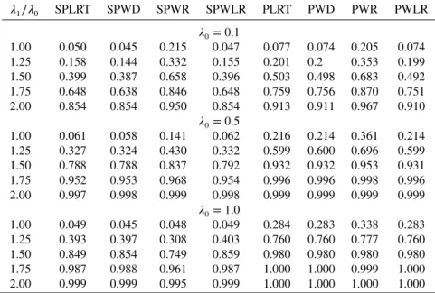
In the second set of simulations, we compare the performance of different tests for testing𝜆₀ = 𝜆₁ under different scenarios. We also consider a na¨ıve method by fitting a Poisson model to the event count data directly. Specifically, we fix the true values of(𝜃,h₀,h₁) at (0.5,0.2,0.2) and vary the values of (𝜆₀, 𝜆₁), as follows:

(a) 𝜆₀=0.1, 𝜆₁=0.1,0.125,0.15,0.175,0.2; (b) 𝜆₀ =0.5, 𝜆₁ =0.5,0.625,0.75,0.875,1.0; and (c) 𝜆₀=1, 𝜆₁=1,1.25,1.5,1.75,2.

Scenario (a) corresponds to the case with rare event, whereas the event of interest is more common under the other two scenarios. The censoring time was set atC = 10 yielding an approximate 25%

Table II.Comparison of the NPMLEs and parametric MLEs.

Semiparametric Parametric

Parameter True Bias SE MSE Bias SE MSE RE

𝜃=0.5,Ha(t) =0.5t0.7

𝛾 2 0.140 0.438 0.211 −0.246 0.330 0.169 0.799

𝜆0 1 −0.003 0.120 0.014 0.083 0.135 0.025 1.753

𝜆1 1 −0.007 0.125 0.016 0.081 0.143 0.027 1.731

𝜃=0.5,H_a(t) =0.5t

𝛾 2 0.133 0.456 0.225 0.092 0.413 0.179 0.796

𝜆0 1 −0.006 0.121 0.015 0.001 0.120 0.014 0.983

𝜆1 1 −0.001 0.119 0.014 0.005 0.119 0.014 0.994

𝜃=0.5,H_a(t) =0.5t1.3

𝛾 2 0.126 0.433 0.203 0.621 0.563 0.702 3.459

𝜆0 1 −0.007 0.121 0.015 −0.064 0.112 0.017 1.137

𝜆1 1 −0.009 0.118 0.014 −0.065 0.110 0.016 1.172

𝜃=1,Ha(t) =0.5t0.7

𝛾 1 0.055 0.172 0.032 −0.106 0.138 0.030 0.932

𝜆0 1 −0.012 0.155 0.024 0.116 0.188 0.049 2.002

𝜆1 1 −0.007 0.158 0.025 0.121 0.194 0.052 2.075

𝜃=1,Ha(t) =0.5t

𝛾 1 0.040 0.169 0.030 0.027 0.160 0.026 0.874

𝜆0 1 −0.007 0.153 0.023 0.001 0.152 0.023 0.984

𝜆1 1 0.000 0.157 0.025 0.010 0.155 0.024 0.990

𝜃=1,H_a(t) =0.5t1.3

𝛾 1 0.050 0.157 0.027 0.212 0.184 0.079 2.924

𝜆0 1 −0.009 0.153 0.024 −0.076 0.142 0.026 1.101

𝜆1 1 −0.007 0.153 0.024 −0.075 0.140 0.025 1.077

Table III. Type I error rate and powers of different tests for testing𝜆₀=𝜆₁based on 1000 replicates withn₀=n₁=100.

𝜆1∕𝜆0 SPLRT SPWD SPWR SPWLR PLRT PWD PWR PWLR

𝜆0=0.1

1.00 0.050 0.045 0.215 0.047 0.077 0.074 0.205 0.074

1.25 0.158 0.144 0.332 0.155 0.201 0.2 0.353 0.199

1.50 0.399 0.387 0.658 0.396 0.503 0.498 0.683 0.492

1.75 0.648 0.638 0.846 0.648 0.759 0.756 0.870 0.751

2.00 0.854 0.854 0.950 0.854 0.913 0.911 0.967 0.910

𝜆0=0.5

1.00 0.061 0.058 0.141 0.062 0.216 0.214 0.361 0.214

1.25 0.327 0.324 0.430 0.332 0.599 0.600 0.696 0.599

1.50 0.788 0.788 0.837 0.792 0.932 0.932 0.953 0.931

1.75 0.952 0.953 0.968 0.954 0.996 0.996 0.998 0.996

2.00 0.997 0.998 0.999 0.998 0.999 0.999 0.999 0.999

𝜆0=1.0

1.00 0.049 0.045 0.048 0.049 0.284 0.283 0.338 0.283

1.25 0.393 0.397 0.308 0.403 0.760 0.760 0.777 0.760

1.50 0.849 0.854 0.749 0.859 0.980 0.980 0.980 0.980

1.75 0.987 0.988 0.961 0.987 1.000 1.000 0.999 1.000

2.00 0.999 0.999 0.995 0.999 1.000 1.000 1.000 1.000

SPLRT refers to the semiparametric likelihood ratio test; SPWD refers to the semiparamet-ric Wald test based on difference of rates; SPWR refers to the semiparametsemiparamet-ric Wald test based on ratio of rates; SPWLR refers to the semiparametric Wald test based on log-ratio of rates; PLRT refers to the parametric likelihood ratio test; PWD refers to the parametric Wald test based on difference of rates; PWR refers to the parametric Wald test based on ratio of rates; and PWLR refers to the parametric Wald test based on log-ratio of rates.

censoring rate. Table III presents the type I error rates and powers of various tests for testingH₀∶𝜆₀=𝜆₁ at significance level of 0.05 based on 1000 replicates withn₀ = n₁ = 100 under scenarios (a)–(c), respectively. In particular, we consider four tests—namely, the likelihood ratio test, the Wald test based on difference of rates, the Wald test based on ratio of rates, and the Wald test based on log-ratio of rates— under both the proposed semiparametric model and the na¨ıve parametric Poisson model. The na¨ıve tests lead to inflated type I error rates especially when the rates are large. The Wald test based on the rate ratio tends to yield inflated type I error rates for rare events and loses power compared with other tests when the event rate is high. All other three tests perform similarly under the semiparametric model.

Finally, we conducted simulation studies to examine the performance of the likelihood ratio test statis-tics for testing𝜃=0, that is, whether there is correlation between the two processes. Figure S1 presents the type I error rates and powers of the likelihood ratio test at significance level of 0.05 based on 1000 replicates withn₀ =n₁ =200 at three different values of𝜆=𝜆₀ =𝜆₁, 0.1, 0.5, and 1.0. The likelihood ratio tests have correct control of the type I error rate and have reasonable powers under the alternative hypotheses.

5. Myelodysplastic syndrome trial

Table IV. Frequencies and relative frequencies of number of events in the MDS trial.

Control Treatment

Count Frequency Proportion Frequency Proportion

0 13 0.26 49 0.49

1 11 0.22 17 0.17

2 3 0.06 2 0.02

3 4 0.08 7 0.07

5 1 0.02 2 0.02

6 1 0.02 4 0.04

7 2 0.04 3 0.03

9 1 0.02 3 0.03

11 1 0.02 3 0.03

12 2 0.04 2 0.02

>12 11 0.22 8 0.08

MDS, myelodysplastic syndrome.

Figure 1.Kaplan–Meier survival curves of the failure time in each treatment group and their 95% confidence bands.

The main objective of the MDS trial is to compare the event rates in the treat group and the placebo group. We now apply the proposed methodology to this data set. For comparison, we also fit a standard Poisson model to the data directly. Table V presents the parameter estimates and their standard errors. The variance of the Gamma frailty is estimated as 1.44 with a standard error of 0.186. There is strong evidence that the event count data and the hazard rate of the dropout time are positively correlated (p-value <1.0×10−10). The na¨ıve method, which does not account for such a correlation, leads to underestimated standard errors of the parameter estimates. Consequently, all four tests described in Section 4 based on the na¨ıve method for testingH₀ ∶𝜆₀ =𝜆₁lead top-values smaller than 0.0001. On the other hand, we obtain non-significant results at𝛼 =0.05 from the likelihood ratio test, the Wald test based on the rate difference, and the Wald test based on the log-ratio of the rates by using the proposed method, withp -values 0.074, 0.081, and 0.052, respectively. The Wald test based on the ratio of the rates has ap-value smaller than 0.0001.

Table V.Results of MDS trial.

Na¨ıve New

Parameter Estimate SE Estimate SE

𝜃 1.443558 0.186276

𝜆0 0.058131 0.003270 0.057941 0.010688

𝜆1 0.033841 0.001711 0.037557 0.004722

MDS, myelodysplastic syndrome; SE, standard error.

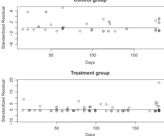
Figure 2.Plot of standardized residuals against follow-up times for the MDS trial.

of HWZ, bootstrapping is used to calculate the standard errors. The method of HWZ yields ap-value of 0.026 for testing the treatment effect. On the other hand, the method of YWH yields a p-value of 2.2×10−10_{for testing the treatment effect. Although the truth is unknown here, as is evident from the} simulation studies, ignoring the correlation between the event count data and dropout time can lead to false positive results, and the Wald statistic based on the ratio of the rates can also lead to false positive results when the event rates are small, which is exactly the case in this application.

Finally, we use a graphical procedure to check the goodness-of-fit of the proposed model. Specifically, we plot the standardized residuals against the follow-up times. As there are no additional covariates in the model, based on equations (3) and (4), the standardized residual for theith subject is calculated as

̂𝜖ni = (Xi− ̂𝜇ni)∕

√ ̂

v_ni,

where

̂𝜇i= (̂𝜃n−1+ Δi)

̂𝜆AinTi

̂𝜃−1

n +ĤAin(Ti)

,

and

̂

v_ni = (̂𝜃_n−1+Ĥ_A

in(Ti) + ̂𝜆AinTi)(̂𝜃 −1

n + Δi)

̂𝜆AinTi

{̂𝜃−1

n +ĤAin(Ti)}2

Figure 3.Plot of standardized residuals against follow-up times for the MDS trial after removing an outlier in the treatment group withXi=45,Ti=180 (days), andΔi=0.

6. Discussion

We have developed a joint semiparametric model for recurrent events data and informative dropout time. This joint model allows one to model these two types of data simultaneously, and the correlation between them is modeled through a Gamma frailty. The proposed method allows one to utilize the additional information in the informative dropout time data to make inference on the event rate. Ignoring such information can lead to invalid inference and inflated type I error rates when comparing the event rates from two groups.

We assumed a gamma shared frailty to account for the correlation between the event count data and the informative dropout time. One advantage of by using the Gamma frailty is that there is a closed form for the observed data likelihood. The joint Gamma frailty model can be easily generalized to different frailty distributions such as the log-normal distribution and the positive stable distribution. However, under these frailty models, the numerical approximations or Monte Carlo approximations are needed to compute the likelihood functions, and hence maximization of the likelihood function is computationally intensive. One drawback of using the shared frailty in models (1) and (2) is that it induces positive correlations, which can be restrictive in practice. Following the idea of [12], we may modify model (2) such that

𝜆(t|𝜉_i,A_i,𝐙i) =𝜉_i𝛼h_A

i(t)exp(𝜻

T_{𝐙i), t∈ [0, 𝜏],}

where𝛼 is an unknown shape parameter. With this modeling, both positive and negative correlations are allowed. However, the likelihood function does not have a closed form except when𝛼is fixed at 1; therefore, it will be computationally more intensive to maximize the likelihood.

In the application, a large portion of the patients had zero events in both the treatment group and the control group. While the proposed method allows for overdispersion in modeling the event count data, it does not handle count data that have an excess of zero counts. We describe a graphical procedure to check the goodness-of-fit of the proposed model through residual plots. It would be desirable to develop formal model diagnostic procedures to examine the goodness-of-fit of the proposed model and further extend the proposed model to event count data with an excess of zero counts. Future research is warranted in this direction.

In model (1), the event rate is proportional to the length of the follow-up time. To improve the flexibility and robustness of the model, we may consider the following semiparametric proportional rate model,

E[N_i(t)|𝜉_i,A_i,𝐙i] =𝜆_A

i𝜉iG(t)exp(𝜷

T_{𝐙i), (6)}

estimate the unspecified baseline mean functionG(⋅)assuming non-informative dropout. Splines provide a smooth estimate of the unknown functions, but they require selection of knots and splines orders. On the other hand, such selection is not needed in the nonparametric maximum likelihood approach. It would be interesting to develop efficient likelihood-based inference procedures for the joint models of (2) and (6). This is a topic of current research.

Appendix A. Regularity conditions

Besides the conditional independent censoring assumption described in Section 2, we impose the following regularity conditions needed for proving Theorems 1–1:

(C1) If there existc₀and𝐜₁such that𝐜T

1𝐙=c0with probability one, thenc0 =0 and𝐜1=𝟎.

(C2) There exists some positive constant number𝛿₀ such thatP(C ⩾ 𝜏|A,𝐙) = P(C = 𝜏|A,𝐙) ⩾ 𝛿₀ almost surely, where𝜏is a constant denoting the end of the study.

(C3) The true parameter values of𝜆₀, 𝜆₁,𝜃,𝜷, and𝜻 belong to a known compact setB₀in(R+₎3_×R2d_.

(C4) The true baseline cumulative distribution functionsH_0a,a=0,1 belong to the following class:

A0 ={Λ ∶ Λis a strictly increasing function in[0, 𝜏]and is continuously differentiable

withΛ(0) =0,Λ′(0)>0 andΛ(𝜏)<∞}.

Appendix B. Proof of Theorem 1

Suppose that two sets of parameters,(𝜆₀,H₀, 𝜆₁,H₁, 𝜃,𝜷,𝜻)and(̃𝜆₀, ̃H₀, ̃𝜆₁, ̃H₁, ̃𝜃, ̃𝜷, ̃𝜻), give the same likelihood function for the observed data, that is,

( 𝜆Ae𝜷

T_𝐙)X{

h_A(T)e𝜻T𝐙

}Δ_Γ(𝜃−1_{+X+ Δ)} Γ(𝜃−1₎

𝜃X+Δ

[

1+𝜃{𝜆_ATe𝜷T𝐙+H_A(T)e𝜻T𝐙}]𝜃 −1_+X+Δ

= (

̃𝜆Ae

̃ 𝜷T

𝐙)X{_h̃

A(T)e

̃ 𝜻T

𝐙}ΔΓ(̃𝜃−1+X+ Δ) Γ(̃𝜃−1₎

̃𝜃X+Δ

[

1+̃𝜃{̃𝜆_ATe𝜷̃T𝐙+H̃_A(T)e𝜻̃T𝐙}

]̃𝜃−1_+X+Δ.

(B.1)

Equation (B.1) holds also for an event count ofX+1. It follows that 𝜆Ae𝜷

T_𝐙 1+𝜃(X+ Δ)

1+𝜃{𝜆_ATe𝜷T𝐙+H_A(T)e𝜻T𝐙} = ̃𝜆Ae ̃ 𝜷T

𝐙 1+̃𝜃(X+ Δ)

1+̃𝜃{̃𝜆_ATe𝜷̃T𝐙+H̃_A(T)e𝜻̃T𝐙}.

(B.2)

The preceding equation holds for bothΔ =0 andΔ =1. Therefore,

1+𝜃(X+1) 1+𝜃X =

1+̃𝜃(X+1) 1+̃𝜃X .

Simple algebra yields𝜃= ̃𝜃. Now letT =0. From Equation (B.2), immediately, we obtain𝜆_Ae𝜷T𝐙 = ̃𝜆Ae𝜷̃

T

𝐙_{. As this equation holds for any𝐙and𝐙}∗_{in the support of the covariates, we obtain𝜷}T_(𝐙−𝐙∗_{) =}

̃

𝜷T

(𝐙−𝐙∗_{). It follows from condition (C1) that𝜷 = 𝜷}̃_{. Then we obtain𝜆}

A = ̃𝜆Afor bothA = 0 and

A = 1. From equation (B.2), we can show thatH_A(t)e𝜻T𝐙 = H̃_A(t)e𝜻̃T𝐙for anyt ∈ [0, 𝜏]and𝐙in its support. Similar techniques and condition (C1) yield𝜻 =𝜻̃ andH_A(t) =H̃_A(t), for anyt ∈ [0, 𝜏]. The identifiability of(𝜆₀,H₀, 𝜆₁,H₁, 𝜃,𝜷,𝜻)is thus established.

Appendix C. Proof of Theorem 2

We introduce some notation that will be used throughout the proof of Theorems 2 and 3. Let𝐎idenote the observations for theith subject consisting of(A_i,X_i,T_i,Δ_i,𝐙i). Let𝐏nand𝐏be the empirical measure and the expectation ofni.i.d. observations𝐎₁,…,𝐎n. That is, for any measurable functiong(𝐎),

𝐏n[g(𝐎)] = 1

n

n

∑

i=1

The proof of consistency consists of two major steps. In the first step, we prove that lim sup_nĤ_an(𝜏),a= 0,1 has an upper bound with probability one. Therefore, there exists a subsequence of(𝝓̂_n, ̂H_0n, ̂H_1n)that converges to(𝝓∗,H₀∗,H₁∗). In the second step, we prove that(𝝓∗,H₀∗,H₁∗) = (𝝓₀,H₀₀,H₁₀).

Step 1. We will prove the uniform boundedness ofĤ_an(𝜏),a = 0,1 by contradiction. Suppose that ̂

H_an(𝜏) → ∞,a = 0,1 in some sample spaceΩ with positive probability. For each sample inΩ, by selecting a subsequence still indexed byn, we assume that𝝓̂_n →𝝓∗andĤ_an(𝜏)→∞,a=0,1. The idea of obtaining a contradiction is as follows: we first construct a step functionH̄_anwith jumps only at the observedT_iin theath group such thatH̄_anis close to the true functionH_a0; then because(𝝓̂_n, ̂H_0n, ̂H_1n) maximizesl_n(𝝓,H₀,H₁), it holds that{l_n(𝝓̂_n, ̂H_0n, ̂H_1n) −l_n(𝝓₀, ̄H_0n, ̄H_1n)}∕n⩾0; finally, we prove that ifĤ_0n(𝜏) → ∞and/orĤ_1n(𝜏) → ∞, the left-hand side of the preceding inequality will eventually be negative, which yields the contradiction.

Recall that the nonparametric log-likelihood takes the form

l_n(𝝓,H₀,H₁) =n𝐏n[R(𝐎;𝝓,H₀,H₁) + ΔlogH_A{T}], where

R(𝐎;𝝓,H₀,H₁) =X(log𝜆_A+𝜷T𝐙) + Δ𝜻T𝐙+

X+Δ−_∑1

k=0

log(𝜃−1+k)

+ (X+ Δ)log𝜃− (𝜃−1+X+ Δ)log{1+𝜃𝜆_ATe𝜷T𝐙+𝜃H_A(T)e𝜻T𝐙}.

By differentiatingl_n(𝝓,H₀,H₁)with respect toH_a{T_i}and setting it to zero, we can see thatĤ_an{T_i} satisfies the following equation.

̂

H_an{T_i} = I(Ai=a)Δi

n𝐏n[I(T⩾t,A=a)Q(𝐎;𝝓̂_n, ̂H_0n, ̂H_1n)] || ||t=Ti

, (C.1)

where

Q(𝐎;𝝓̂_n, ̂H_0n, ̂H_1n) = (1+ ̂𝜃nX+ ̂𝜃nΔ)e ̂ 𝜻T

n𝐙

1+̂𝜃_n̂𝜆_Ane𝜷̂Tn𝐙+ ̂𝜃

nĤAn(T)e

̂ 𝜻T

n𝐙

.

In view of (C.1), we construct another step functionH̄_an(t)with jumps only at the observedT_iin the

ath group and the jump size satisfies that ̄

H_an{T_i} = I(Ai=a)Δi

n𝐏n[I(T⩾t,A=a)Q(𝐎;𝝓₀,H₀₀,H₀₁)]||||t=Ti

. (C.2)

We verify thatH̄_an(t)converges toH_0auniformly int ∈ [0, 𝜏]with probability one. It can be shown that the class

Fa = {I(T⩾t,A=a)Q(t,𝐎;𝝓,H0,H1) ∶t∈ [0, 𝜏],(𝜆0, 𝜆1, 𝜃,𝜷,𝜻) ∈B0,Ha∈A,Ha(0) =0}

is a bounded and P-Donsker class, where

A= {g∶gis a nondecreasing function in[0, 𝜏],g(𝜏)⩽B₀} andB₀is a positive constant based on condition (C5).

As a P-Donsker class is also a Glivenko–Cantelli class, by the Glivenko–Cantelli theorem in [35], ̄

H_an(t)uniformly converges to

E[I(T⩽t,A=a)Δ∕𝜇_a(T)], where𝜇_a(t) =E[I(T⩾t,A=a)Q(𝐎;𝝓₀,H₀₀,H₀₁)].

By the conditional independent censoring assumption (C1) and with some tedious algebra, we can prove that

As(𝝓̂_n, ̂H_0n, ̂H_1n)maximizesl_n(𝝓,H₀,H₁),

0⩽1

nln(𝝓̂n, ̂H0n, ̂H1n) −

1

nln(𝝓0, ̄H0n, ̄H1n).

By plugging Ĥ_an{T_i} of equation (C.1) and H̄_an{T_i} of equation (C.2) into l_n(𝝓̂_n, ̂H_0n, ̂H_1n) and

l_n(𝝓₀, ̄H_0n, ̄H_1n), respectively, we obtain

0⩽1

n

n

∑

i=1 1 ∑

a=0

I(A_i=a) [

− Δ_ilog

{ 1

n

n

∑

j=1

I(T_j⩾T_i,A_j=a)Q(𝐎j;𝝓̂_n, ̂H_0n, ̂H_1n) }

+R(𝐎i;𝝓̂_n, ̂H_0n, ̂H_1n) −R(𝐎i;𝝓₀, ̄H_0n, ̄H_1n)

+ Δ_ilog

{ 1

n

n

∑

j=1

I(T_j⩾T_i,A_j=a)Q(𝐎j;𝝓₀,H₀₀,H₁₀) } ]

⩽O(1) − 1

n

n

∑

i=1 1 ∑

a=0

I(A_i=a) [

Δ_ilog

{ 1

n

n

∑

j=1

I(T_j⩾T_i,A_j=a)

g₁+Ĥ_an(T_j) }

+ (̂𝜃−_n1+X_i+ Δ_i)log {

1+̂𝜃_n̂𝜆_anT_ie𝜷̂

T n𝐙i₊̂𝜃

nĤan(Ti)e

̂ 𝜻T

n𝐙i

} ] ,

(C.3)

whereg₁is some positive constant. The last inequality above is obtained from conditions (C4) and (C5). Recall that ̂𝜃_nconverges to𝜃∗_{. If𝜃}∗_{=0, and we can show that the right-hand side of inequality (C.3)}

diverges to negative infinity asĤ_0n(𝜏) → ∞orĤ_1n(𝜏) → ∞. We have the contradiction because the left-hand side is non-negative. Therefore, we assume that𝜃∗_{>0. It follows that}

0⩽O(1) −1

n

n

∑

i=1 1 ∑

a=0

I(A_i=a) [

Δ_ilog

{ 1

n

n

∑

j=1

I(T_j⩾T_i,A_j=a)

g₁+Ĥ_an(T_j) }

+ (g₂+ Δ_i)log{g₃+Ĥ_an(T_i)} ],

(C.4)

for some positive constantsg₂andg₃.

We will show that ifĤ_0n(𝜏)→ ∞orĤ_1n(𝜏)→ ∞, the right-hand side of (C.4) diverges to−∞. We mimic the arguments of Murphy [29] to prove the divergence of the right-hand side. Specifically, for both

a=0 anda=1, we choose a partition of[0, 𝜏], as follows: withs₀=𝜏, chooses₁ <s₀such that 1

2E{(g2+ Δi)I(Ti=s0,Ai=a)}>E{ΔiI(Ti∈ [s1,s0),Ai=a)}. By conditions (C2) and (C3), suchs₁exists. We next define a constant𝜖∈ (0,1)such that

𝜖

g₂(1−𝜖) <

E{I(T_i∈ [s₁,s₀),A_i=a)}

E{Δ_iI(T_i∈ [0, 𝜏),A_i=a)}.

Ifs₁>0, we can chooses₂=max(0,s)such thatsis the minimum value less thans₁satisfying that (1−𝜖)E{(g₂+ Δ_i)I(T_i∈ [s₁,s₀),A_i=a)}⩾E{Δ_iI(T_i∈ [s,s₁),A_i=a)}.

Clearly,s₂exists under the regularity conditions, ands₂<s₁. This process can continue so that we obtain a sequence𝜏=s₀>s₁>s₂>· · ·⩾0 such that

1

Such a sequence cannot be infinite, that is, there exists a finiteNsuch thats_N+1=0; otherwise,s_q→s∗

for somes∗_{[0, 𝜏). By the definition ofs}

q, it holds that

(1−𝜖)E{(g₂+ Δ_i)I(T_i∈ [s_q,s_q−1),A_i=a)} =E{Δ_iI(T_I∈ [s_q+1,s_q),A_i=a)}, q⩾1. By the continuity of true densities, we sum overq=1,2,…and obtain

(1−𝜖)E{(g₂+ Δ_i)I(T_i ∈ [s∗, 𝜏),A_i=a)} =E{Δ_iI(T_i∈ [s∗,s₁),A_i=a)}. Thus,

g₂(1−𝜖)E{I(T_i∈ [s∗, 𝜏),A_i=a)}⩽𝜖E{Δ_iI(T_i∈ [s∗,s₁),A_i=a)},

which contradicts with the choice of𝜖. Therefore, the sequence is finite:𝜏 =s₀ >s₁ >· · ·>s_N+1 =0. Therefore, the right-hand side of (C.4) can be bounded from above by

O(1) −1

n

n

∑

i=1 1 ∑

a=0

I(A_i=a) [

(g₂+ Δ_i)I(T_i=𝜏)log{g₃+Ĥ_an(𝜏)}

+

N

∑

q=0

(g₂+ Δ_i)I(T_i∈ [s_q+1,s_q))log{g₃+Ĥ_an(s_q+1)}

+

N

∑

q=0

Δ_iI(T_i∈ [s_q+1,s_q))log {

1

n

n

∑

j=1

I(T_j⩾T_i,A_j=a,T_j∈ [s_q+1,s_q))

g₁+Ĥ_an(s_q)

} ]

⩽O(1) −1

n

n

∑

i=1 1 ∑

a=0

I(A_i=a) [

1

2(g2+ Δi)I(Ti=𝜏)log{g3+Ĥan(𝜏)} +

{ 1

2(g2+ Δi)I(Ti=𝜏)log{g3+Ĥan(𝜏)} − ΔiI(Ti∈ [s1,s0))log{g3+Ĥan(𝜏)} }

+

N

∑

q=1 {

(g₂+ Δ_i)I(T_i∈ [s_q,s_q−1))log{g₃+Ĥ_an(s_q)}

− Δ_iI(T_i∈ [s_q+1,s_q))log{g₃+Ĥ_an(s_q)} }

+

N

∑

q=0

Δ_iI(T_i∈ [s_q+1,s_q))log {

1

n

n

∑

j=1

I(T_j⩾T_i,T_j∈ [s_q+1,s_q)) } ]

.

(C.5)

The first term on the right-hand side of (C.5) diverges to−∞asĤ_0n(𝜏)→∞orĤ_1n →∞. The second term is negative for largenowing to the choice ofs₁. By the selection ofs_q,q = 1,…,N, the third term cannot diverge to∞. Finally, the fourth term is bounded because of the Glivenko–Cantelli theorem. Hence, the right-hand side of (C.5) diverges to−∞. This contradicts the fact that the left-hand side of (C.5) is non-negative. Therefore, we have shown that, with probability one,Ĥ_an(𝜏),a=0,1 is bounded for any sample sizen.

Thus, by Helly’s selection theorem, we can choose a further subsequence, still indexed by{n}, such that(̂𝜆_0n, ̂H_0n, ̂𝜆_1n, ̂H_1n, ̂𝜃_n, ̂𝜷_n, ̂𝜻_n)converges to(𝜆∗

0,H

∗

0, 𝜆

∗

1,H

∗

1, 𝜃

∗_,𝜷∗_,𝜻∗_{)with probability one.}

Step 2.In this step, we will show that

(𝜆∗₀,H∗₀, 𝜆∗₁,H₁∗, 𝜃∗,𝜷∗,𝜻∗) = (𝜆₀₀,H₀₀, 𝜆₁₀,H₁₀, 𝜃₀,𝜷₀,𝜻₀).

We useĤ_an(t)andH̄_an(t)in step 1. By the construction ofĤ_an(t)andH̄_an(t), we can see thatĤ_an(t)is absolutely continuous with respect toH̄_an(t)and

̂

H_an(t) = ∫

t

0

Pn[I(T⩾y,A=a)Q(y,𝐎;𝝓0,H00,H01)]

Pn[I(T⩾y,A=a)Q(y,𝐎;𝝓̂n, ̂H0n, ̂H1n)]

By taking limits on both sides of (C.6), we obtain that

H_a∗(t) = ∫

t

0

P[I(T⩾y,A=a)Q(y,𝐎;𝝓₀,H₀₀,H₀₁)]

P[I(T⩾y,A=a)Q(y,𝐎;𝝓∗,H∗

0,H

∗

1)]

dH_0a(y).

Therefore,H∗

a(t)is differentiable with respect toH0a(t)so thatH∗a(t)is differentiable with respect tot. It

follows thatdĤ_an(t)∕dH̄_an(t)converges todH∗

a(t)∕dH0a(t)uniformly int∈ [0, 𝜏].

Note that

n−1l_n(̂𝜆_0n, ̂H_0n, ̂𝜆_1n, ̂H_1n, ̂𝜃_n) −n−1l_n(𝜆₀₀, ̄H_0n, 𝜆₀₁, ̄H_1n, 𝜃₀)

=P_n

[

ΔlogĤAn{T}

̄

H_An{T} ]

+P_n[R(𝐎; ̂𝜆_0n, ̂H_0n, ̂𝜆_1n, ̂H_1n, ̂𝜃_n) −R(𝐎;𝜆₀₀, ̄H_0n, 𝜆₀₁, ̄H_1n, 𝜃₀)] ⩾0.

(C.7)

AsB₀×Ais a Donsker class and the functionalsR(𝐎;𝝓,H₀,H₁)are bounded Lipschitz functionals with respect toB₀×A, the following class

F2 = {R(𝐎;𝝓,H0,H1) ∶ (𝜆0, 𝜆1, 𝜃,𝜷,𝜻) ∈B0,Ha ∈A,Ha(0) =0,Ha(𝜏)⩽B0,a=0,1} is P-Donsker and hence a Glivenko–Cantelli class. Therefore, by lettingn→∞in (C.7), we have

0⩽P [

log { _h∗

A(T)

Δ_eR(𝐎;𝝓∗_,H∗

0,H

∗

1) h_A0(T)Δ_eR(𝐎;𝝓0,H00,H01)

}] ,

which is the negative Kullback–Leibler information. Then it follows that, with probability one,

h∗_A(T)ΔeR(𝐎;𝝓∗,H∗0,H

∗

1)=h

A0(T)ΔeR(𝐎;𝝓0,H00,H01).

Therefore, from the identifiability result proved earlier, we obtain(𝝓∗,H₀∗,H₁∗) = (𝝓₀,H₀₀,H₀₁). This completes the proof of Theorem 2. Note that the uniform convergence ofĤ_antoH_a0,a= 0,1 follows from the fact thatH_a0are continuous functions.

Appendix D. Proof of Theorem 3

We prove Theorem 3 by verifying the four conditions in Theorem 3.3.1 of [35]. For this purpose, we first define a neighborhood of the true parameters(𝝓₀,H₀,H₁), denoted by

U= {(𝝓,H₀,H₁) ∶||𝝓−𝝓₀||+ sup

t∈[0,𝜏]

(|H₀(t) −H₀₀(t)|+|H₁(t) −H₀₁(t)|)< 𝜖₀},

for a very small constant 𝜖₀. Based on the consistency theorem, (𝝓̂_n, ̂H_0n, ̂H_1n) belongs to U with probability close to 1 when the sample sizenis large enough.

For any one-dimensional submodel given as {𝜆₀ +𝜖h₁, 𝜆₁ +𝜖h₂, 𝜃 +𝜖h₃,𝜷+𝜖𝐡₄,𝜻 +𝜖𝐡₅,H₀ + 𝜖∫ h₆dH₀,H₁+𝜖∫ h₇dH₁},(𝝓,H₀,H₁) ∈U,𝐇≡(h₁,h₂,h₃,𝐡₄,𝐡₅,h₆,h₇) ∈H, we can derive the score function for a single observation𝐎

W(𝐎;𝝓,H₀,H₁)[𝐇] =l_𝜆

0(𝝓,H0,H1)h1+l𝜆1(𝝓,H0,H1)h2+l𝜃(𝝓,H0,H1)h3

+l_𝛽(𝝓,H₀,H₁)T𝐡₄+l_𝜁(𝝓,H₀,H₁)T𝐡₅

+l_H

0(𝝓,H0,H1)

[

∫ h6dH0 ]

+l_H

1(𝝓,H0,H1)

[

∫ h7dH1 ]

,

(D.1)

where

l_𝜆

a(𝐎;𝝓,H0,H1) =I(A=a)

{

X

𝜆a

− (1+𝜃X+𝜃Δ)Te

𝜷T_𝐙

1+𝜃𝜆_aTe𝜷T𝐙+𝜃H_a(T)e𝜻T𝐙

}