C
2013. The American Astronomical Society. All rights reserved. Printed in the U.S.A.
EXTINCTION AND POLYCYCLIC AROMATIC HYDROCARBON INTENSITY VARIATIONS
ACROSS THE H
ii
REGION IRAS 12063
−
6259
D. J. Stock1, E. Peeters1,2, A. G. G. M. Tielens3, J. N. Otaguro1, and A. Bik4 1Department of Physics and Astronomy, University of Western Ontario, London, ON N6A 3K7, Canada
2SETI Institute, 189 Bernardo Avenue, Suite 100, Mountain View, CA 94043, USA 3Leiden Observatory, Leiden University, P.O. Box 9513, NL-2300 RA Leiden, The Netherlands
4Max-Planck-Institut f¨ur Astronomie, K¨onigstuhl 17, D-69117 Heidelberg, Germany Received 2013 April 2; accepted 2013 May 21; published 2013 June 17
ABSTRACT
The spatial variations in polycyclic aromatic hydrocarbon (PAH) band intensities are normally attributed to the physical conditions of the emitting PAHs, however in recent years it has been suggested that such variations are caused mainly by extinction. To resolve this question, we have obtained near-infrared (NIR), mid-infrared (MIR), and radio observations of the compact Hii region IRAS 12063−6259. We use these data to construct multiple independent extinction maps and also to measure the main PAH features (6.2, 7.7, 8.6, and 11.2 μm) in the MIR. Three extinction maps are derived: the first using the NIR hydrogen lines and case B recombination theory; the second combining the NIR data with radio data; and the third making use of the Spitzer/IRS MIR observations to measure the 9.8μm silicate absorption feature using the Spoon method and PAHFIT (as the depth of this feature can be related to overall extinction). The silicate absorption over the bright, southern component of IRAS 12063−6259 is almost absent while the other methods find significant extinction. While such breakdowns of the relationship between the NIR extinction and the 9.8μm absorption have been observed in molecular clouds, they have never been observed for Hiiregions. We then compare the PAH intensity variations in theSpitzer/IRS data after dereddening to those found in the original data. It was found that in most cases, the PAH band intensity variations persist even after dereddening, implying that extinction is not the main cause of the PAH band intensity variations.
Key words: dust, extinction – galaxies: ISM – Hii regions – infrared: ISM – ISM: lines and bands – ISM: molecules
Online-only material:color figures
1. INTRODUCTION
The mid-infrared (MIR) spectra of many Galactic and extra-galactic sources display the well-known unidentified infrared bands at 3.3, 6.2, 7.7, 8.6, 11.2, and 12.7 μm (see Gillett et al. 1973; Geballe et al. 1989; Cohen et al. 1989). These broad emission features are generally attributed to the infrared (IR) relaxation of UV-pumped polycyclic aromatic hydrocarbon (PAH) molecules (Puget & L´eger1989; Allamandola et al.1989; Tielens2008).
Observationally, the relative strengths, peak position, and pro-file of the PAH features have been seen to vary considerably within a source and from source to source (e.g., Peeters et al.
2002a; Hony et al. 2001; van Diedenhoven et al. 2004). The relative strengths of PAH features also change drastically go-ing from neutral molecules to ions in laboratory studies (see Allamandola et al.1999). In particular, the 3.3 and 11.2μm features arise primarily from neutral PAH molecules while the 6.2, 7.7, and 8.6μm features are attributed to PAH ions. This allows ratios involving the neutrals and ions, such as the 7.7/11.2 ratio, to be useful tools for probing the ionization state of the emitting molecules and hence for probing the local phys-ical conditions (e.g., Galliano et al.2008). In addition, smaller molecules dominate the emission at shorter wavelengths while larger molecules emit predominantly at longer wavelengths (Allamandola et al.1989; Schutte et al.1993).
Despite the success of PAH ratios as tracers of physical conditions within a source, dust extinction often hampers
measuring and interpreting these ratios. While there is extinction across the whole IR range, the main issue for PAHs is silicate extinction in the MIR which primarily affects the 8.6 and 11.2μm PAH bands. Moreover, this extinction can vary spatially across a source, complicating the interpretation of the observed MIR PAH features. Galliano et al. (2008) investigated variations in the PAH ratios in a variety of objects including M82, and concluded that PAH variations are being caused by the properties of the emitting PAH population within the objects in their study. However, Beir˜ao et al. (2008) attribute the PAH band variations in this source to extinction variations. Indeed they posited that the variations in dust extinction are strong enough to affect the interpretation of their calculated PAH ratios, which showed variations comparable to the variations in extinction.
This presents a fundamental problem in interpreting PAH ratios: are the variations in the band ratios intrinsic to the source? Are they the direct result of variations in the extinction due to dust? Or are they some combination of the two? Unfortunately, the only source in which this effect has been studied, M82, is a very complex and distant source, so eachSpitzer/Infrared Spectrograph (IRS) pixel contains unresolved structure which adds to the already considerable uncertainties on the extinction and PAH measurements. On the other hand, many Galactic Hii
other methods of extinction measurement. As a result, studying the effects of extinction on PAH variations in a Galactic Hii
region instead of M82 should result in a prime testbed to address this question.
Understanding the characteristics of dust in regions of mas-sive star formation is of key importance as dust extinction and reemission dominates the spectral energy distribution (SED) of these regions. Studies on the properties of dust in Hiiregions around massive young stars have a long history dating back to the optical studies on light scattering by Mathis et al. (1977), IR studies by Wynn-Williams et al. (1972), and submillime-ter Westbrook et al. (1976). The advent of moderate resolu-tion IR spectrometers with wide coverage on ground-based and space based platforms has opened up novel ways of probing the dust characteristics in Hiiregions through comparisons of the strength of IR recombination lines and studies of this type have revealed distinct differences with dust properties in the dif-fuse ISM (e.g., Lutz et al.1996). The absorption characteristics of dust in Hiiregions can also be gleaned from detailed studies of the (IR) SED (Salgado et al.2012; Sreenilayam & Fich2011; Kirk et al.2010). The high sensitivity of the IRS spectrometer on theSpitzer Space Telescopehas opened up the study of the characteristics of dust in molecular clouds through photometric and spectroscopic studies of background stars shining through the cloud (Chiar et al.2007,2011; van Breemen et al.2011; Boogert et al. 2011). These observations reveal that the dust properties vary widely within molecular clouds and regions of star formation. These variations likely reflect the importance of coagulation of interstellar dust in larger and larger aggregates as the density increases (Ormel et al.2007; Ossenkopf & Henning
1994).
There are several well known ways to measure the extinction in an Hiiregion of which three will be employed in this paper. The first two require observations of the ionized hydrogen emission from the center of the Hii region. We will employ the recombination lines in the near-infrared (NIR) and this shall be referred to as the NIR method. The second method, the radio method, involves comparing the strength of the NIR hydrogen lines with the radio continuum generated by the same ionized hydrogen. The third method is independent of the first two, and fits the 9.8μm silicate profile to the observed spectra, deriving the depth of the 9.8μm silicate absorption feature; this will be referred to as the “Spoon” method (Spoon et al.2007). In addition, the code PAHFIT does a similar analysis to the Spoon method in fitting the MIR spectrum and provides the optical depth of the 9.8μm silicate absorption feature.
We have therefore obtained narrow band photometric ob-servations of the Paschen β (hereafter Paβ) and Brackett γ
(hereafter Brγ) hydrogen lines of the Galactic Hii region (IRAS 12063−6259, He 2–77). We will combine these data with MIRSpitzer/IRS spectral maps and radio to create mul-tiple extinction maps to ensure consistency. Subsequently, we can use these extinction maps to correct ourSpitzer/IRS obser-vations in order to investigate the effects of extinction on the PAH band ratios.
Section2 will be devoted to background information about IRAS 12063−6259, including the relevant prior observations. In Section3the data reduction processes relevant to the ISAAC, Australia Telescope Compact Array (ATCA) andSpitzer/IRS data are described. Section4shows the derivations of extinc-tion maps from these data along with relevant discussion. In Section5, the measurement of the PAH bands and their cor-relations in the reddened and dereddened data are presented.
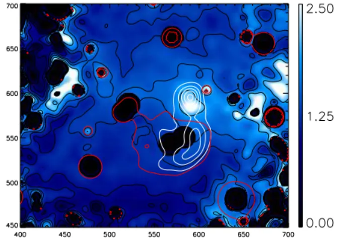
Figure 1.Three color image of IRAS 12063−6259 with 8.6 GHz radio contours
(Mart´ın-Hern´andez et al.2003) overlain in black with the two radio sources A and B indicated. The image covers an area of 1by 1, the red and green data are the background subtracted ISAAC 2.17μm Brγand 1.28μm Paβobservations respectively and blue represents Hαfrom the SHS (Southern Hemisphere Hα
Survey; Parker et al.2005). TheISO-SWS aperture is shown in white and the IRS-SL cube field of view is shown in red. North is up and east is to the left. The dark circles are masked out areas around field stars. The dark lane across the center of the nebulosity is consistent with the observations of strong silicate 9.8μm absorption in that area (see Section4.3).
(A color version of this figure is available in the online journal.)
In Section 5, the morphology of IRAS 12063−6259 and the effects of extinction on PAHs is discussed and Section6presents conclusions.
2. IRAS 12063−6259
IRAS 12063−6259, an ultra compact Hiiregion at a distance of 10 kpc (Caswell & Haynes 1987), was first classified as a possible planetary nebula (PN) by Henize (1967). The first suggestions that it was perhaps not a PN were prompted by inspection of the SED in which the 10 μm photometry was consistent with silicate absorption—suggesting that it was an Hiiregion (Cohen & Barlow1980). This mis-classification is, in some ways, fortunate though, as its inclusion in PNe catalogs has provided abundances based on optical spectroscopy (e.g., Kingsburgh & Barlow1994). It was also observed in the radio in PNe surveys, revealing a very bright object at 5 GHz (Milne
1979).
Further radio observations by Mart´ın-Hern´andez et al. (2003) using the ATA array at 4.8 and 8.6 GHz indicate separation into three distinct sources, A and B with the B source further divided into B1 and B2 (A: 12:09:01.12 −63:15:52.9; B: 12:09:01.01 −63:16:00.8). It is thought that this separation reflects the likely stellar content—i.e., a cluster of three stars rather than a single ionizing star. We show an optical/NIR image of IRAS 12063−6259 in Figure1with radio contours. The dark lane in the center of Figure1indicates a high degree of extinction.
Table 1
Log of Observations (a) VLT/ISAAC
Filter Date Integration Time AB Target Seeing
DIT×NDIT Cycles ()
1.21μm 2010 Feb 28 3.6 s×39 5 IRAS 12063−6259 0.71
1.21μm 2010 Feb 28 3.6 s×8 5 HD 115115
1.28μm 2010 Mar 1 3.6 s×12 5 IRAS 12063−6259 1.53
1.28μm 2010 Mar 1 3.6 s×8 5 HD 115115
2.17μm 2010 Mar 1 3.6 s×39 5 IRAS 12063−6259 0.94
2.17μm 2010 Mar 1 3.6 s×8 5 HD 115115
2.19μm 2010 Mar 1 3.6 s×12 5 IRAS 12063−6259 0.83
2.19μm 2010 Mar 1 3.6 s×8 5 HD 115115
(b)Spitzer/IRS
Date Cycles× Pointings Step Size
Ramp Time (s) ⊥ () ⊥
2006 Mar 19 20×6.29 1 7 3.0 3.6
(c) ATCAb
Frequency Configuration Date Integration Time
(GHz) (minutes)
4.8 6D 2000 Apr 9 80
8.64 6D 2000 Apr 9 80
4.8 1.5D 2000 Apr 11 80
8.64 1.5D 2000 Apr 11 80
Notes.
aα, δ(J2000); units ofαare hours, minutes, and seconds, and units ofδare degrees, arc minutes, and arc seconds. bSee Mart´ın-Hern´andez et al. (2003) for details.
at the same location as the brightest patch of nebulosity in Hα, Paβ, and Brγ. The optical/NIR image shows this band most clearly, particularly the Hαimage. This feature is evident in the extinction maps, particularly in the NIR case B recombination map and partially in the MIR silicate feature maps. It is clear that the dark band is caused by extinction, rather than a lack of flux in the shorter wavelength filters, because the band obscures the continuum radio emission from the radio A Hiiregion.
The extinction band is also present in Two Micron All Sky Survey (2MASS)JHKsimages, which closely match the morphology of the Hαimage presented in Figure1. In the long wavelength (8.6μm)Spitzer/IRAC images the dark lane present in optical/NIR data is absent and we see bright IR sources at the positions of both radio A and B. However, the radio A source is substantially fainter at 3.6μm than the radio B source(s). This observation is in agreement with the optical/NIR conclusion that source A suffers from very high extinction.
Spectroscopic observations in the optical and NIR have yielded nebular conditions and abundances. Electron densi-ties have been derived using both IR and optical methods. Kingsburgh & Barlow (1994) found a density of 3000 ± 1050 cm−3 using the optical [Sii] doublet. The IR [Oiii] 88/52 μm lines loosely agree, yielding a value of 1335+484−284 cm−3 (Mart´ın-Hern´andez et al.2002). There are few
tempera-ture estimates of this object because heavy extinction in the op-tical obscures the standard temperature sensitive lines. Caswell & Haynes (1987) found a value of 6400 K using observations of NIR hydrogen lines, however they noted that this value was uncorrected with respect to galactocentric radius and its effect on metallicity and therefore temperature. Kingsburgh & Barlow (1994) performed the correction and foundTe=8800 K. This
figure was found to agree with the Te = 9000 K found by
Jourdain de Muizon et al. (1987) based on the ratio of [Siii] 6312 Å and 18.7μm fluxes.
3. OBSERVATIONS AND DATA REDUCTION
3.1. ISAAC Data Reduction
IRAS 12063−6259 was observed using the ISAAC instru-ment (Moorwood et al. 1998) on UT3 (Melipal) of the Very Large Telescope (VLT, program ID: 084.C-0569). A complete log of our ISAAC observations is presented in Table1(a). Paβ
and Brγ narrow band filters at 1.27 and 2.17 μm were em-ployed to observe the emission line intensities across the neb-ula. Observations were also performed using adjacent narrow band filters (1.21, 2.19μm) in order to measure the continuum component of the nebular emission. A standard star at similar airmass (HD 115115) was observed in the same narrow-band filters subsequent to the observation of the Hiiregion.
These ISAAC observations were performed in nodding/
jittering configuration, allowing optimal removal of the sky background for both the nebular and standard star images by the ESO reduction pipeline. Each science frame was dark subtracted and flat-fielded using calibration data obtained that evening. The ISAAC data reduction pipeline was found to produce images with slightly offset World Coordinate System (WCS) information to the order of 5–10 in each reduction. The images were subsequently aligned by selecting stars with known WCS coordinates from the 2MASS point source catalog and adjusting the WCS information of each frame to match these coordinates.
For example:
F1∗.21 FJ∗ =
1.21+
1.21−f(λ)S1.21(λ)dλ
J+
J−f(λ)SJ(λ)dλ
, (1)
whereF1∗.21/F∗
J is the ratio of fluxes expected between the two filters, 1.21−and 1.21+ are the upper and lower limits of the 1.21 μm narrow band filter, f(λ) is the flux of the star as a function of wavelength andS(λ) is the filter profile as a function of wavelength.
Using this relationship, the standard star flux can then be related to the observed counts to obtain the flux per count necessary for calibration of our science images. In each case, the standard star was observed at roughly the same airmass as the science target and immediately following the science observation. The airmass corrections were integrated into the process of determining the flux per count.
The choice of standard star was constrained heavily by airmass and position on the sky constraints, as such we have checked our calibration by repeating this process for each star in both standard and object fields for which we have both photometry and 2MASS magnitudes. This assumed that most stars in both fields are likely to be late-type and therefore differences in their SEDs are likely to be minor and will not influence the calibration. In this process, we carefully excluded outliers, which were either (1) embedded within the source, (2) either optical doubles or visual binaries for which the ISAAC pipeline had incorrectly measured the counts, or (3) early type stars. It was also necessary to remove stars with high 2MASS magnitudes (11), as our observations are much more sensitive than those of 2MASS and this introduces nonlinearities at very low count levels. Fits to this data provide the flux per count and allow us to calibrate our images. The fits for each filter are consistent with those derived using just the standard star.
Table1(a) also lists the seeing for each image as derived from the point-spread functions (PSFs) of the stars in the field by the ESO ISAAC pipeline. Unfortunately, one of the set of four images of IRAS 12063−6259 (1.28 μm) has approximately double the seeing (1.5) of the other images (0.7–0.9). In order to compensate, we smoothed the three other images to match the seeing of the worst image (Brγ). The four images of the source were then calibrated, and images of Brγ and Paβ created by subtracting the adjacent background images (1.21 and 2.19μm respectively).
Following the calibration process, the field stars in the images were masked to prevent them from influencing later science results.
The signal-to-noise ratio (S/N) of the resulting Brγ and Paβ
maps varies across IR 12063. Both achieve a S/N of greater than 10 pixel−1in the area around radio B, but the area around radio A is more variable, with the S/N of Paβand Brγdropping to around 0.5 and 5 pixel−1respectively.
3.2. Spitzer/IRS Data Reduction
IRAS 12063−6259 was observed with the short–low (SL) module of the IRS (Houck et al. 2004) on-board the Spitzer Space Telescope(PID: 20517, AOR: 14798848). We have sum-marized these observations in Table1(b). Both the first (SL1, 7.4–14.5μm, 1.8 pixel−1) and the second (SL2, 5.2–7.7μm, 1.8 pixel−1) orders were used to create a spectral map, with spectral resolutionsλ/δλ between 64 and 128. These
observa-tions cover an area of 57×26(see the red box in Figure1). The PSF is about 2 pixels, roughly 3.6.
The spectral mapping data obtained were processed through the pipeline reduction software at the Spitzer Science Cen-ter (Version 18.18). The BCD images were cleaned using CUBISM (Smith et al.2007a), wherein any rogue or otherwise “bad” pixels were masked, first using the built in “AutoGen Global Bad Pixels” with settings “Sigma-Trim”=7, “MinBad-Frac” =0.5 and “AutoGen Record Bad Pixels” with settings “Sigma-Trim”=7 and “MinBad-Frac”=0.75 and subsequently by manual inspection of each cube. Cleaned data cubes corre-sponding to each spectral order were made in this way. Finally, the SL2 spectra were scaled to match the SL1 spectra in order to correct for the mismatches between the two order segments. The bonus order SL3 was used to determine the scaling factors, since it overlaps slightly with both SL1 and SL2. These scaling factors were typically 5%, well in agreement with the typical values of 10% obtained by Smith et al. (2007b). Spectra were extracted from the spectral maps by moving, in 1 pixel steps, a spectral aperture of 2×2 pixels in both directions of the maps. This results in overlapping extraction apertures.
Before measuring PAH fluxes in the IRS spectral cube, the continuum was removed from each spectrum by computing a spline polynomial fit to the continuum (including a point at 8.2 μm) and then subtracting the spline (see, e.g., Hony et al.2001; Peeters et al.2002a). The most prominent features were measured by integrating all of the remaining flux between fixed points, e.g., 5.86–6.6 μm for the 6.2 μm feature. The 7.7μm complex was also measured using this method, while the weaker features (6.0, 11.0μm) were fitted with Gaussians. For 6.0 and 11.0 these were then subtracted from the 6.2 and 11.2μm fluxes to compensate for their inclusion in the initial integration. The 12.7 μm feature appears blended with the 12.8μm [Neiii] line along with the 12.3μm H2line, all of which
were fitted concurrently in order to minimize uncertainties. For the Gaussian fits, uncertainties are generated in the fitting process, while for the features for which the integration was used, uncertainties were calculated by measuring the rms noise in various wavelength windows and then combining this with each flux measurement to find the S/N.
3.3. ATCA Data Reduction
Mart´ın-Hern´andez et al. (2003) observed IRAS 12063−6259 using the ATCA (Program C868) in 2000 April/May using the 6 km (6D) and 1.5 km (1.5D) configurations at 4.8 and 8.6 GHz. Details of the reduction of this dataset are discussed by Mart´ın-Hern´andez et al. (2003). A log of the relevant observations is shown in Table1(c). The configuration of the ATCA array used for these observations means that sensitivity drops off away from the source and very little extended structure is detected.
4. RESULTS AND ANALYSIS
4.1. NIR Hydrogen Lines
The general formula for differential extinction Aλ1 −Aλ2
between two different wavelengthsλ1andλ2is given by:
Aλ1−Aλ2= −2.5×
log
F(λ1)
F(λ2)
−log
F0(λ1)
F0(λ2)
, (2)
whereF0(λ1) is the intrinsic flux andF(λ1) is the observed flux of a line atλ1. Given an electron density of 1000–3000 cm−3and
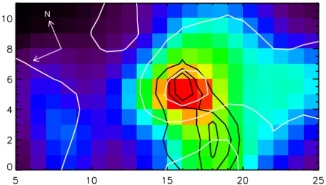
Figure 2.Extinction map derived using case B recombination assumptions and ISAAC narrow band hydrogen line images. Black contours representAK of
0.25, 0.5, 0.75, 1.0, 1.25, 1.5, 2; white contours represent the 4.8 GHz radio observations (as in Figure1). The red contours surrounding radio B and some bright stars represent the PaβS/N level of 3. Solid black circles represent areas in which foreground stars have been masked out. Thexandyaxes refer to positions in pixels on the NIR images (0.148 pixel−1).
(A color version of this figure is available in the online journal.)
Storey (1987) gives (F0(Paβ)/F0(Brγ)) = 5.82. Equation (2)
can then be restated for this specific case as:
APaβ−ABrγ = −2.5×log
F(Paβ) 5.82×F(Brγ)
. (3)
Extinction in the NIR (∼1–3 μm) is described by a power law, usually taken to be of the following form (Mathis1990; Martin & Whittet1990):
Aλ= AK
(λ/2.2)α, (4)
whereλis inμm and the exponentαis usually in the range of 1.7–2.0 for the ISM (e.g., Martin & Whittet1990).
It is then possible to state bothAPaβandABrγ in terms ofAK
by substituting Equation (4) as appropriate:
AK = −
2.5 1.62×log
F(Paβ) 5.82×F(Brγ)
, (5)
adoptingα=1.8 (e.g., Mart´ın-Hern´andez et al.2002).
Upon substitution of our flux calibrated maps, this produces the extinction map shown in Figure 2. The area of highest extinction is correlated with the dark lane across the nebula (Figure1). The highest extinction values (AK ∼2) are observed
at the same position as the radio A source (and as such are compromised by a lack of signal to noise), the second radio source (radio B) is obscured to a much lower extent (AK ∼1–1.5).
The derived values ofAK (0.6–2.5) are consistent with the
average value of 0.8 derived by Mart´ın-Hern´andez et al. (2002) usingISO-SWS data. The Mart´ın-Hern´andez et al. (2002) value would be biased toward the lower values as theInfrared Space Observatory(ISO) aperture (14×20, see Figure 2 of Mart´ın-Hern´andez et al.2003) included the brightest (lowest extinction) parts which dominate the emission line spectrum and lead to a lower overall estimate of extinction.
This method will henceforth be referred to as the NIR method.
4.2. Radio Continuum and Near-IR Hydrogen Lines
From radio observations of the ionized hydrogen continuum at multiple frequencies it is possible to derive the intrinsic in-tensity of recombination lines that are also emitted. This can be used to measure extinction as the observed flux of a hydro-gen line (such as those discussed in the previous section) can be compared to the flux predicted by the radio observations. In order to derive the flux implied by the radio observations, some other quantities (such as the electron temperature and emission measure (EM)) must also be derived. Using the ATCA radio observations (discussed in Section 3.3) a brightness tempera-ture map for both 4.8 and 8.6 GHz observations can be calcu-lated. The brightness temperature is defined as (Tielens2005, Equation (7.70)):
Sν =
2ν2
c2 kTBΩ, (6)
whereνis the frequency in Hz,TBis the brightness temperature
in K, andΩis the source solid angle. The source solid angle has been explicitly included to facilitate the creation of brightness temperature maps (i.e., per pixel), rather than the usual method of using the sum of all radio flux for the whole object.
We can rearrange to find:
TB =3.26×10⁻⁵× Sν
ν2GHzΩ (K). (7)
We will refer to the maps created using this equation as the “observed” brightness temperature maps. The brightness temperatures are in general much higher for the 4.8 GHz map, peaking at around 300 K as opposed to 50 K for the 8.64 GHz map.
The unusual configuration of the ATCA array means that the ATCA beam is an elliptical rather than a circular aperture. As it is necessary to combine the two maps, they were combined by smoothing the higher frequency (8.64 GHz) map using the larger beam of the low frequency (4.8 GHz) map, taking into account this ellipticity.
The following equations then describe the relationship be-tween the important quantities necessary for calculating the intrinsic emission of any hydrogen recombination line, namely the electron temperature,Teand EM:
TB=Te(1−e−τ(ν)) (K) (8)
and:
τ(ν)=(8.235×10⁻²)aTe−1.35
ν GHz
−2.1 EM
cm−6pc
, (9)
whereνis the frequency of our radio observations,τ(ν) is the optical depth for that frequency andais a function ofTeandν
and represents the ratio of the true optical depth to a simplified approximation (Mezger & Henderson1967).
Te was then found using iterative calculations (see Watson
et al. 1997; Osterbrock & Ferland 2006) after combining Equations (8) and (9) to find:
TB,4.8 =Te
1−e−τ8.64×[84..648]
−2.1
(K), (10)
where TB,4.8 is the observed 4.8 GHz brightness temperature
map and the factorτ8.64×[4.8/8.64]−2.1represents the optical
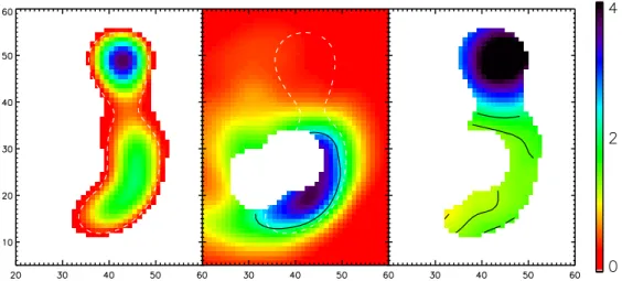
Figure 3.Predicted map of the Brγflux derived from ATCA radio observations (left, white dashed contour at 1.5×10⁻¹³erg s−1cm−2); Brγflux observed with ISAAC smoothed to approximately the same resolution as the radio data, where the white region is a masked out star (middle, black contour represents 5×10⁻¹⁴erg s−1cm−2), white contours are those of the data in the left panel) and theAKmap resulting from Equation (15) (right, contours atAK =0.5, 1, 2, 3). The colorbar to the right
refers exclusively to the image in the right panel. For each panel, thexandyaxes are positions in pixels on the radio image (0.3 pixel−1). (A color version of this figure is available in the online journal.)
For the first iteration, the temperatures measured by previous authors (as mentioned in Section2) of around 9000 K was used for the whole map. The difference between the observed bright-ness temperature map and that calculated using Equation (10) was applied iteratively to correct ourTe map until no further
changes were observed. The resultant map shows that radio A has a slightly lower average temperature (∼8000 K) than radio B (9000 K) and that the temperature throughout most of the emission is roughly constant at around 9000 K. KnowingTe,
Equation (9) can then be rearranged to calculate the EM for each pixel:
EM=4.72a−1Te1.35
ν GHz
2.1
τ(ν) (cm−5). (11)
Following Watson et al. (1997), we then calculate the ex-pected flux at Brγusing the following equation:
SBrγ =0.9hνBrγαeffBrγ Ω
4πEM (erg cm
−2s−1), (12)
where it is assumed that the hydrogen abundance by number is 0.9,h is Planck’s constant, νBrγ is the frequency of a Brγ
photon,Ωis the solid angle subtended by the emitting source and
αBreffγ =(6.48×10⁻¹¹)Te−1.06 (13)
represents the effective recombination cross section (Hummer & Storey1987).
To find a specific expression for SBrγ, we can substitute
Equation (11) into Equation (12) to yield:
SBrγ =4.24hνBrγαeffBrγν2 .1 4.8 GHz
Ω
4πT
0.29
e τ(ν) (erg cm−2s−1),
(14)
which was calculated for each pixel of the map. The extinc-tion ABrγ, is then calculated by comparing the observed and
calculated Brγ fluxes (Equation (15)).
ABrγ = −2.5×log
SBrγ
SBrγ ,0
. (15)
From this, theKband extinction,AK, is found as before, using
Equation (4). The calculated Brγmap (Equation (14)), is shown along with the observed ISAAC Brγmap smoothed to the same resolution, in Figure3, along with the resultant extinction map. This method will be referred to as the radio method.
4.3. Mid-IR Silicate Absorption
Spoon et al. (2007) proposed a method for measuring the depth of the 9.8μm silicate absorption feature independent of any intrinsic profile of the absorption. The Spoon method, for PAH dominated spectra (see Spoon et al.2007), is as follows: interpolate a power law continuum using points at 5.5μm and 14.5μm of the formy =axk, then calculate the natural log of
the ratio of the flux of this continuum at 9.8μm and the observed flux at 9.8μm. This value, calledSsil by Spoon et al. (2007), can be interpreted as the optical depth at 9.8μm,τ9.8μm. An
example of this method employed on theSpitzer/IRS spectra of radio A and B is presented in Figure4.
As discussed by Brandl et al. (2006), if significant silicate extinction is present, the flux of the long wavelength continuum point will be affected by absorption because of the overlapping of the 9.8 and 18μm bands. Brandl et al. (2006) suggest that if a long–low (LL) IRS cube is available, that the 14.5 μm continuum point can be abandoned in favor of one at 23 μm which is less susceptible to silicate absorption. LL data for IRAS 12063−6259 are not available, so a new approach, iteratively calculating the extinction using the Spoon method in combination with a wavelength profile of the absorption, has been devised.
When the 14.5 μm continuum point is affected by silicate absorption, the Spoon method underestimates the continuum at 9.8 μm—leading to an underprediction of τ9.8. Dereddening
such IRS spectra using this value of τ9.8, will still leave
unaccounted for silicate absorption (this is shown in Figure4, where the dashed red line is the result of dereddening the radio A spectrum in this way). The new method implemented here applies the Spoon method again to such a dereddened spectrum, to find a new value ofτ9.8. This process of applying
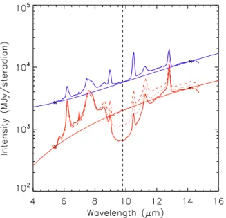
Figure 4.Example of the Spoon method (Spoon et al.2007) usingSpitzer/IRS spectra. The red and blue lines represent theSpitzer/IRS SL spectra of radio A (iterative SpoonAK=2.3; SpoonAK=0.0) and B (iterative SpoonAK=0.0)
respectively. The radio B spectrum has been offset from the radio A spectrum for clarity. The thin red and blue lines are the initial interpolated power law continua for both cases (with the interpolation points marked with crosses), the black dashed line atλ=9.8μm shows the approximate location of the silicate feature. The red dotted and dashed lines are the spectrum of radio A after being dereddened using the non-iterative Spoon method (dotted) and the iterative Spoon method (dashed) and then normalized to the observed spectrum. (A color version of this figure is available in the online journal.)
is then compared with the observed 9.8μm flux in the original spectrum. For the spectra most affected by silicate absorption (τ9.8 >2.0), the difference between the initial value provided
by the Spoon method and the final value was around 40%. In practice, the Chiar & Tielens (2006) description of the shape of the 9.8 and 18μm silicate extinction features in the ISM is used to deredden the IRS SL spectra at each stage. The Chiar & Tielens (2006) model also gives a direct relation-ship betweenA9.8andAK, which turns out to be nearly equal to
one (1.006). This provides the following relation betweenτ9.8
andAK:
AK = A9.8
1.006 =
1.086×τ9.8
1.006 =1.079×τ9.8. (16)
So to within 10%,AK is equal toτ9.8 under the conditions
for which the Chiar & Tielens (2006) description of the silicate features in the local ISM are satisfied. This method will be referred to as the Spoon method in future discussion. The map of extinction as measured by the Spoon method is presented in Figure5.
4.4. Comparisons between Extinction Maps
Before using the various extinction maps to deredden MIR observations, they can be compared for consistency and corre-lations. In each case, the higher spatial resolution observation must be binned to match the resolution of the lower and then the derived extinctions for each pixel can be compared. The three maps have pixels of size 0.15, 0.3, and 1.8 for the NIR, radio, and IRS data respectively. As such, S/N improves significantly upon binning. However, it is still likely that many NIR points will be untrustworthy as (1) the native resolution measurements of Paβwhich are used to create them are have very low S/N and
Figure 5.Map of the 9.8μm silicate absorption as measured by the Spoon
method. White contours represent 4.8 GHz brightness temperature 50, 100, 150 K. Thexandyaxes refer to positions in pixels on the IRS cube (1.8 pixel−1). (A color version of this figure is available in the online journal.)
Figure 6.ISAACAK(resampled to the same resolution as the radio data) against
radioAK. The cluster of points are those from the radio B Hiiregion.
(2) the morphology of the NIR narrow band emission does not match that of the MIR or radio emission. Point b also applies to the radio method, as the Brγ image is used for this method. Morphologically, the only large scale comparison can be drawn between the NIR map and the Spoon map as they cover large areas. The NIR map (Figure2) shows the prominent bar (AK=
1.5–2) running from east to west, with the highest extinction (AK=2.5) occurring very near to the location of radio A within
the bar. The southern regions, near radio B but also covering the extended emission evident in the Hαmap shown in Figure1, display anAKof between 1 and 1.25. In contrast, the Spoon map
(Figure5) shows zero extinction in the southern regions near radio B. It agrees with the NIR map in that the peak extinction occurs near radio A (although it underestimates the degree of extinction), but the “bar” of extinction visible in the NIR is only somewhat present as it falls between the radio A peak and the large region of silicate absorption occurring to the east.
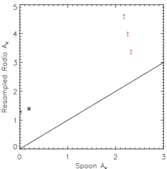
Figure 7.SpoonAK against radioAK (resampled to Spitzer/IRS SL pixel
size: 1.8). High extinction points are associated with the pixels associated with radio A, while the low extinction points are from radio B.
(A color version of this figure is available in the online journal.)
the high extinction radio A source as there is very little Paβflux in this region.
Figure7shows the correlation between the extinction derived from the radio data against that derived using the Spoon method. The high extinction points near radio A have been included as lower limits (see later discussion). At lowAK(radio B), the radio
method presents a value of around 1.4, while the Spoon method finds a value very close to zero (<0.2).
In Figure8, the correlation between the extinction derived from the NIR method versus that derived using the Spoon method is shown. Figure8includes all of the data for the region surrounding IRAS 12063−6259 in Figure8as both theSpitzer/
IRS map and the ISAAC data are valid away from the brightest regions of the source. In Figure8, the points associated with the radio B Hiiregion have been indicated (red points) and all possess lower Spoon extinction than those away from the radio B Hiiregion (blue points) as is already obvious from a cursory inspection of the spectra (see Figure4). In Figure 8, the S/N threshold for including points was increased to 5 to better display the discrepancy between the area of low silicate absorption near radio B and the higher absorption in the surroundings. In principle the radio method is the most accurate at measuring the total extinction between the emitting source and the observer. The radio observations detect the total emission from the Hii
region and so reflect the true shape of the ionized region, while at Brγ the morphology is more complex and does not totally match that in the radio. Around radio B, the Brγ and radio morphologies match and the extinction measured is the same as that of the NIR method. However near radio A, it is debatable whether any of the detected Brγ flux emanates from the radio A Hiiregion at all. The morphology of the emission is certainly very different, indicating the possibility that this may be diffuse emission associated with IR 12063 or foreground emission. In that case, the extinction derived from the Brγ-radio continuum comparison provides a lower limit to the extinction of source A (and an upper limit to the extinction associated with the surrounding diffuse Hiicomponent). Near radio B, a consistent extinction is found with the NIR and the radio methods, but
Figure 8.SpoonAK against ISAACAK. The radio B pixels from Figure7
are marked as black crosses, the remaining points are included as blue or red diamonds corresponding to regions away from or associated with the radio B Hii
region (i.e., within the southern low extinction region in Figure5) respectively. (A color version of this figure is available in the online journal.)
a discrepant extinction, of around AK ∼ 0.2, is found using
the Spoon method. The emission morphology around radio B is very similar in the radio and NIR, so we can safely assume that the extinctions measured are the extinction between the radio B Hiiregion and the observer for the ISAAC and radio methods. The discrepant measurement arising from the Spoon method around radio B was checked using an independent measure of the silicate absorption feature: PAHFIT (Smith et al.2007b).
Both methods agree that the pixels coincident with radio B, marked with red diamonds in Figure9, have low silicate optical depths (τ9.8<0.5) in agreement with the Spoon method, while
the bulk of the rest of the points display much higher silicate absorption. At low optical depths, the points in Figure9seem to agree, while at higher optical depths (>1) PAHFIT finds a higher optical depth (by around a factor of two) than the Spoon method. Beir˜ao et al. (2008) found the opposite trend in that they quote a higher range of values for the Spoon method rather than PAHFIT.
PAHFIT was used to measure each pixel of the IRS-SL cube of IRAS 12063−6259, and the resulting correlation between theτ9.8 of PAHFIT against that of the Spoon method is shown
in Figure 9. It should be noted that PAHFIT is intended to fit full IRS spectra (5–40μm), and large uncertainties result from using PAHFIT with only the IRS/SL range (5–14μm) because the longer wavelength continuum greatly aids the fitting process. However there exist no longer wavelength observations of IRAS 12063−6259 so the silicate absorption strength as measured by PAHFIT result from its application to only the IRS/SL range. In order to achieve a sensible extinction result from PAHFIT, it was necessary to impose a floor ofτ9.8=0.01
because it was found that PAHFIT frequently found fits to many of the pixels in the map with zero silicate absorption, even for pixels where the Spoon method found considerable optical depth (up toτ9.8(Spoon) ∼ 2). Even after imposing this floor, there
is still evidence of this effect in Figure9, where there is a line of points atτ9.8(PAHFIT)=0.01 and a range of Spoon values
Figure 9.Spoonτ9.8against PAHFITτ9.8. The pixels from radio B have been
indicated with filled red diamonds. The black line indicates a 1:1 correlation. (A color version of this figure is available in the online journal.)
where the Spoon method detects optical depths of 0.8. From Figure9 we can also see the opposite effect, there are some pixels in which PAHFIT detects optical depths of up to 0.8 where the Spoon method detects zero optical depth, so it seems that under low optical depth conditions, both methods carry large uncertainties.
In the diffuse ISM, the 9.8 μm optical depth (as provided by the Spoon method) and extinction derived in the NIR have been found to follow a tight correlation (e.g., Whittet 2003, and references therein). Hints that there may be a different relationship between these quantities in some circumstances, i.e., possibly a shallower correlation, were found by Whittet et al. (1988). Later studies confirmed this difference for molecular cloud sightlines and found that both the 9.8μm silicate optical depth, and the total optical depth at 9.8 μm (continuum + silicates) correlate well with the NIR extinction, albeit with a shallower dependence for molecular clouds than the diffuse ISM (e.g., Chiar et al.2007,2011; McClure2009; van Breemen et al.2011). The data and correlations from these studies, along with that of IRAS 12063−6259 are shown in Figure10. None of the aforementioned studies found objects as extreme as radio B (NIRAK =1.5, τ9.8 =0.2). The areas of diffuse emission
around the radio B Hii region are slightly above the general ISM trend (NIRAK ∼1.5,τ9.8∼1.0; blue points in Figure8).
In Figure10, a selection of Hiiregions have been included which were present in the Mart´ın-Hern´andez et al. (2002) sample and so have NIRAKmeasurements. The corresponding
measurements of their silicate optical depth were found by applying the Spoon method5to theirISO-SWS spectra (Peeters
et al.2002b). The large ISO-SWS beam means that both the
5 In this case the Spoon method was not applied iteratively, in order to match the measurement process of other data shown in Figure10.
Figure 10.Comparison ofτ9.8(Spoon) and NIR extinction with reference points
representing the diffuse ISM and molecular clouds (black crosses; Chiar et al.
2011), a sample of Hiiregions observed withISO-SWS (Peeters et al.2002b; black triangles, see text) and the measurements of the area around radio B and the diffuse emission from around IRAS 12063−6259 (red diamonds and blue diamonds respectively, the same points as in Figure8). Best fit lines for ISM and molecular cloud sightlines are shown in black.
(A color version of this figure is available in the online journal.)
NIRAK’s and silicate optical depths are spatial averages across
each Hii region. In general the ISO-SWS Hii region sample appear along the ISM trend in Figure10. However three of them: IRAS 02219+6152, IRAS 10589−6034 and IRAS 18434−0242 (better known as G029.96−00.02), appear in roughly the same place as radio B in Figure 10. IRAS 10589−6034 is part of a larger complex of very bright Hα emission (saturated in the Southern Hemisphere HαSurvey (SHS)) and also appears with similar morphology in each of the 2MASS bands. These points are much lower than either the molecular cloud or ISM trends. The three sources mentioned all have higher values of τ9.8 shown in the literature (e.g., Hackwell et al. 1978
for IRAS 02219+6152) however, there is very little trace of absorption in theISO-SWS spectra.
From inspection of Figure 10, it appears that Hii regions follow the ISM trend when spatially integrated but that under certain circumstances they can violate this trend and have low silicate absorption. In the case of IRAS 12063−6259, the radio B points appear to follow the molecular cloud trend while the diffuse surroundings follow the diffuse ISM trend. The three sources which appear near the radio B points in Figure 10
Figure 11.Map of the 6.2μm PAH emission. Black contours represent 4.8 GHz brightness temperature 50, 100, 150 K; white contours represent the silicate absorption as measured by the Spoon method, peaking at radio A. Thexandy axes refer to positions in pixels on the IRS cube (1.8 pixel−1).
(A color version of this figure is available in the online journal.)
possibly the observations of the other Hiiregions) represents a combination of both effects and as such the IRAS 12063−6259 point appears near, but below, the DISM trend in Figure10.
The physical interpretation of the differing relationship be-tweenτ9.7 and the NIR extinction is usually attributed to the
effects of grain growth in molecular clouds. Grain coagulation causes the NIR opacity to rise relative to the 9.8μm silicate absorption because silicates are more easily coagulated than carbonaceous material. While van Breemen et al. (2011) found that it was very difficult to reproduce the observed relation-ship betweenτ9.7 and the NIR extinction without significantly
altering the shape of the 9.8μm feature profile, the shape of the 9.8μm silicate absorption feature in the vicinity of radio B cannot be directly measured as there is so little absorption (see Figure4). The other major possibility which could solve the discrepancy between the NIR extinction and the silicate op-tical depth is that properties of the NIR extinction, generated by carbonaceous materials is different in the vicinity of radio B. This possibility can be ruled out on the grounds that the radio and NIR extinction measurements appear to be consistent with standard NIR extinction laws (e.g., Equation (4)).
The preceding discussion dramatically alters the picture of how the extinction maps can be applied to dereddening the MIR cube. It appears that each extinction map is valid in somewhat different regions. The NIR extinction map, for example is only valid around radio B, where there is sufficient S/N to make an accurate determination of the extinction. The radio extinction map is also only accurate around radio B, and over a much smaller area than the NIR map (because the radio observations are not sensitive to structure on larger scales). The Spoon and PAHFIT maps appear to not be trustworthy in the vicinity of radio A or B, as the previous discussion has shown that the ratio of silicate absorption to NIR extinction around both is much lower than would be expected.
4.5. PAH Band Ratio Variations and Extinction
In order to investigate the effects of extinction on the ratios of the major PAH bands, the IRS cube (as described in Section3.2) was dereddened using the Chiar & Tielens (2006) prescription for the extinction in the MIR relative toAKusing the extinction
maps described in the previous section. The regions for which the extinction maps are not thought to be trustworthy have been removed and are not presented in the following analysis.
The continuum subtraction and flux measuring process as described in Section 3.2 was repeated for cubes dereddened
Figure 12. Map of the 8.6 μm PAH emission. Black contours: 4.8 GHz
brightness temperature 50, 100, 150 K; white contours represent silicate absorption as measured by the Spoon method, peaking at radio A. Thexandy axes refer to positions in pixels on the IRS cube (1.8 pixel−1).
(A color version of this figure is available in the online journal.)
using the Spoon and NIR methods in the areas of their validity. In this section the unaltered observations will be referred to as the “observed” data, while the dereddened data will be referred to by the extinction map which was used to create it, e.g., Spoon or NIR.
Following the discussion in Section4.4, the extinction maps were used for dereddening in areas where they are valid. Therefore, in the case of the Spoon extinction map, the area around both radio sources is likely untrustworthy and has been masked out. For the NIR map, only the regions where the Paβ
signal to noise is above three at native resolution are included. The radio extinction map has not been used for dereddening purposes as it covers a very small area and would produce very few dereddened points.
The spatial distributions of the PAH bands (shown in Figures11and12) show strong spatial variations which seem to correlate with extinction. The 6.2 and 7.7 μm bands peak in absolute strength near radio A as well as being very simi-lar morphologically (see Figure11for 6.2μm map along with radio and silicate absorption contours). In both maps the radio A peaks are all slightly offset to the south of radio A, possibly attributable to the large gradient in extinction in this region. They also show additional emission extending west toward the edge of the map. The 6.2 and 7.7μm maps also display isolated weak emission east of radio A. The 8.6 and 11.2 μm bands peak around radio B and also share the same morphology, with some extended emission toward radio A. Figure12shows the morphology of the 8.6μm emission, as compared to the radio emission and the strength of silicate absorption. A comparison of Figures11and12shows the effects of the silicate absorp-tion band on PAHs in that the morphologies are dramatically different. The area around radio A, associated with the highest extinction values, has strong 6.2 and 7.7μm and weak 8.6 and 11.2μm emission.
In general, ratios of PAH band intensities (i.e., I6.2/I11.2)
are taken to remove any influence that distance, abundance, or variations in the intrinsic strength of the whole PAH spectrum may play on the relationships between the bands. This allows unbiased inspection of the relative strengths of different bands. The most commonly quoted correlation, I6.2/I11.2 versus
I7.7/I11.2, is presented in Figure 13. Similar trends are seen
for both I8.6/I11.2 versus I7.7/I11.2 (Figure 14) and I8.6/I11.2
versusI6.2/I11.2 (Figure15) in the observed data. Fits to each
Table 2
Parameters of PAH Intensity Ratio Correlations
Data Slope Intercept SlopeY(0)=0 Correlation Coefficient
I6.2/I11.2vs.I7.7/I11.2
Observed 3.19±0.06 −0.60±0.11 2.84±0.01 0.961
Spoon 2.27±0.06 0.53±0.07 2.72±0.01 0.947
NIR 3.66±0.26 −1.19±0.25 2.47±0.03 0.914
NGC 2023a 2.04±0.02 −0.29±0.03 1.89±0.01 0.967
M17b 1.96 0.81
I8.6/I11.2vs.I7.7/I11.2
Observed 5.24±0.15 −1.71±0.19 3.90±0.03 0.954
Spoon 17.01±3.37 −12.77±3.17 3.42±0.03 0.636
NIR 2.17±0.18 0.97±0.13 3.57±0.08 0.871
NGC 2023a 4.40±0.06 1.17±0.03 6.31±0.04 0.953
M17b . . . 11.91 0.33
I8.6/I11.2vs.I6.2/I11.2
Observed 1.66±0.07 −0.38±0.09 1.37±0.01 0.880
Spoon 10.19±2.82 −8.40±2.65 1.25±0.01 0.593
NIR 0.41±0.08 0.70±0.06 1.43±0.05 0.676
NGC 2023a 2.13±0.03 0.72±0.03 3.44±0.02 0.949
Notes.
aE. Peeters et al. (2013, in preparation). bGalliano et al. (2008).
Figure 13.I6.2/I11.2plotted againstI7.7/I11.2for the pixels surrounding radio A
and B. The red triangles represent the observed ratios while the blue diamonds represent the same data after dereddening using the Spoon extinction map and the green squares are similar using the ISAAC extinction map. Best fit gradients for each set of points are shown in the same color. A dereddening vector corresponding toAK=1 is shown in black.
(A color version of this figure is available in the online journal.)
Separate gradients for each correlation are provided which pass through the origin or are allowed to vary theiry-intercepts.
In each of Figures13–15dereddened points have also been included. For the I6.2/I11.2 versus I7.7/I11.2 correlation, the
points with the highest ordinate values correspond to the points of highest extinction around radio A. This collection of points (I7.7/I11.2 > 5) clearly displays a different slope than the rest
of the points for the low extinction parts of the source. The dereddened points in Figure13remove the “break” in the slopes evident in the observed data.
The general effect of extinction of the I6.2/I11.2 versus
I7.7/I11.2 correlation is most straightforward to explain: the
Figure 14.I8,6/I11.2plotted againstI7.7/I11.2for the pixels surrounding radio
A and B. The red, blue, and green points are as in Figure13. Best fit gradients for each set of points are shown in the same color. A dereddening vector corresponding toAK=1 is shown in black.
(A color version of this figure is available in the online journal.)
11.2μm PAH band is affected by extinction from the 9.8μm silicate feature to a greater degree than the 6.2 or 7.7μm bands. Therefore the effect of extinction is to preferentially reduce the 11.2μm PAH flux and increase both theI6.2/I11.2andI7.7/I11.2
ratios. The major effect of dereddening this correlation is to decrease each of the ratios and as such move all points toward the origin.
Figure 15.I8.6/I11.2plotted againstI6.2/I11.2for the pixels surrounding radio A and B. The red, blue, and green points are as in Figure13. Best fit gradients for each set of points are shown in the same color. A dereddening vector corresponding toAK=1 is shown in black.
(A color version of this figure is available in the online journal.)
IRAS 12063−6259 and NGC 2023. Included in Table2 are the correlations derived by Galliano et al. (2008) for the M17 galactic star formation complex, which is the only galactic Hii region in the Galliano et al. (2008) sample. The M17 correlation for I6.2/I11.2 versus I7.7/I11.2 gives a lower value
than the 2.846found for the non-dereddened IRAS 12063−6259
data. The values found for IRAS 12063−6259 are lowered by the dereddening process to as low as 2.42, however this still significantly differs. Nevertheless, even after dereddening a tight correlation exists the IRAS 12063−6259 data.
The other correlations listed in Table 2 also disagree with those for NGC 2023 and M17, however in these cases the effect of dereddening, as discussed above, does not narrow the gap between the IRAS 12063−6259 data and that of the other objects. The two dereddening methods employed twist the best fit correlations in opposite ways, i.e., for the map dereddened using the Spoon method the gradient increases drastically (by a factor of 3–6). While the NIR dereddened data yields a shallower best fit, giving reductions in the gradients by a factor of 2–3. From inspection of the correlation plots (Figures14and15) this appears to be because the Spoon method collapses the variation in theI8.6/I11.2ratio to around one, while the NIR method gives
a range from around 0.2 to 1.2.
In Figure 16, another commonly examined correlation
I6.2/I7.7 versusI11.2/I7.7 is shown, which is considered to be
a useful diagnostic of PAH size and ionization (Draine & Li 2001). The tracks for ionized and neutral PAHs at vary-ing Nc are adopted from Draine & Li (2001). The observed
IRAS 12063−6259 points fall between the tracks, indicating a mixture of ionized and neutral PAHs, albeit at the lowest end of theNcvalues considered (Nc=16!). However it is clear that
the dereddening process has significantly altered theI11.2/I7.7
ratio, as might be expected given thatAλ/
AKat 11.2μm is higher than the other PAH bands. In fact, dereddening has increased
6 Galliano et al. (2008) quote only gradients for correlations which pass through the origin, so the quoted gradient is for the IRAS 12063−6259 correlation defined in the same way.
Figure 16. I6.2/I7.7 vs.I11.2/I7.7 for the area around IRAS 12063−6259.
The red, blue, and green points are as in Figure13. The two lines represent ionized (lower) and neutral (upper) PAH tracks for a variety of PAH molecule sizes (increasing toward the left; Draine & Li2001). A dereddening vector corresponding toAK=1 is shown in black.
(A color version of this figure is available in the online journal.)
Figure 17. I7.7/I11.2 plotted against I12.7/I11.2 for the area around
IRAS 12063−6259. The red, blue, and green points are as in Figure13. A dereddening vector corresponding toAK=1 is shown in black.
(A color version of this figure is available in the online journal.)
the range of values ofI11.2/I7.7from∼0.15 to around 0.3. The
range of values inI6.2/I7.7does not change significantly as the
difference betweenAλ/
AK at 6.2 and 7.7μm are much smaller. In addition to the main bands, the 12.7μm band was measured as it should also be weakly affected by extinction. In Figure17
the observed I6.2/I11.2 versusI12.7/I11.2 correlation is shown,
along with the dereddened versions as in previous figures. The ratio ofI12.7/I11.2 is of particular note as its variation
de-creases the most after dereddening. Dereddening via the Spoon method in particular reduces variation in theI12.7/I11.2 ratio to
5. DISCUSSION
5.1. The Morphology and Geometry of IRAS 12063−6259
The somewhat conflicting extinction maps suggest a geom-etry for IRAS 12063−6259: radio A is actually a deeply em-bedded, highly extinguished Hiiregion separated from the Hii
region around radio B. The PAH bands are seen to sharply peak at the same position as radio A, which strongly argues for most of the emitting PAHs being located in the photodissociation region around the radio A Hiiregion and not associated with the extended PAH emission evident in the Figure11. In this case, the radio A PAH emission should suffer from a similar level of extinction as the ionized part of the Hii region, yet the MIR spectra reveal only modest silicate absorption. The fact that the Spoon method finds a much lower extinction (at least a factor of two) than the lower limit given by the radio method is possibly another instance of the expected relation-ship between the NIR extinction and the silicate absorption breaking down.
The radio B source, on the other hand, suffers from a similar problem which we must tentatively attribute to silicate coagulation. The non zero NIR extinction and near zero silicate optical depth are difficult to explain using other mechanisms especially as the NIR extinction around radio B is consistent with standard extinction laws. Radio B appears to have cast off its extinguishing material (possibly due to it being a small cluster of stars as suggested by Mart´ın-Hern´andez et al.2003). It is also possible that radio B is simply older and has cast off its natal cloud. Given the lack of extinguishing material on our line of sight, it seems that the stars making up radio B are the likely cause of the extended PAH emission surrounding IRAS 12063−6259.
5.2. Methods of Measuring Extinction
Here we discuss the possible ramifications of our findings regarding the various methods of measuring extinction. It is important to note that each method, in isolation, presents a seemingly reliable measurement of extinction. It is only when compared to other independent measures of extinction that inconsistencies emerge.
The Spoon method is commonly used to classify external galaxies (e.g., Spoon et al.2007). In this role it provides a self-consistent way of determining the degree of silicate absorption, albeit not a very accurate in terms of the total extinction as it seems to systematically underestimate the degree of silicate optical depth (as shown in Section4.3where we developed a method of compensating for this effect). In addition, it does not seem to be linked to the overall extinction, as measured by the radio method, as has also been concluded from completely independent methods to measure the extinction associated with molecular cloud materials (e.g., Chiar et al.2007,2011; McClure2009; van Breemen et al.2011).
Spatial extinction maps also show that different regions of a small object can have vastly different extinction properties. If we regard theISO-SWS spectra of IRAS 12063−6259 as an average of the whole object, it shows some silicate absorption as well as NIR extinction. TheSpitzer/IRS observations disentangle these two effects and show that they are spatially distinct on scales of the 0.4 pc separation between the two radio sources. In the case of IRAS 12063−6259, this small separation is resolved, for the usual application of the Spoon method (galaxy classification) variations on this scale will be entirely invisible.
5.3. PAH Variations and Extinction
The primary argument made by Beir˜ao et al. (2008) was that because the variations in PAH band ratios were lower than the variations one would expect due to variations in the ex-tinction; one could not reliably ascribe these variations to any other cause. Beir˜ao et al. (2008) made this assertion based on the scatter in their plot of I6.2/I7.7 against I11.2/I7.7 (which
we show with our data in Figure16), which was rather close to the expected dereddening vector. For IRAS 12063−6259, it is observed that the range of points on this figure is main-tained or even amplified upon dereddening (regardless of the extinction map chosen). This implies that the variations in the PAH band ratios are not due to variable extinction but are intrinsic.
We find that correlations involving the 8.6 μm band are highly affected by extinction, as one might expect. However the combination of the band being weak and the second most heavily affected by extinction produce very scattered correlation plots (e.g., Figures14and15) with low correlation coefficients. This probably also arises from the uncertainty on the wavelength profile of the 9.8μm silicate absorption feature which has been found to vary significantly (van Breemen et al. 2011). The different extinction maps used to deredden the IRS cube have the largest effect on the 8.6/11.2 PAH ratio. The data dereddened using the Spoon map shows much lower dispersion than that dereddened using the NIR map. There are three potential explanations for this effect, it could be a reflection of the NIR extinction map being noisier than the Spoon map, although if this were the case it would be expected that the NIR points on the correlation plots would have a higher scatter without preferring any specific direction, which is not observed. Second, it could be that the method of using an extinction law to measure extinction and then dereddening using the same extinction law introduces biases which cause the Spoon dereddened points to cluster. Last, it could be that the Spoon method systematically fails at lowAK,
in this case the points at low extinction do not move at all (as for low NIRAKthe Spoon method seems to findAK=0) while
the high extinction points move toward them—decreasing the scatter. However, the agreement between the Spoon method and PAHFIT on the lack of absorption in radio B spectra seems to rule out the final possibility being a systematic error and suggest that instead, the 8.6/11.2 PAH ratio displays a lower variation than expected.