The dust properties and physical conditions of the interstellar medium
in the LMC massive star-forming complex N11
M. Galametz,
1‹S. Hony,
2M. Albrecht,
3F. Galliano,
4D. Cormier,
2V. Lebouteiller,
4M. Y. Lee,
4S. C. Madden,
4A. Bolatto,
5C. Bot,
6A. Hughes,
7F. Israel,
8M. Meixner,
9,10J. M. Oliviera,
11D. Paradis,
7,12E. Pellegrini,
2,13J. Roman-Duval,
9M. Rubio,
14M. Sewiło,
15,16Y. Fukui,
17A. Kawamura
17and T. Onishi
18Affiliations are listed at the end of the paper
Accepted 2015 November 23. Received 2015 November 9; in original form 2015 August 4
A B S T R A C T
We combineSpitzerandHerscheldata of the star-forming region N11 in the Large Magellanic Cloud (LMC) to produce detailed maps of the dust properties in the complex and study their variations with the interstellar-medium conditions. We also compare Atacama Pathfinder EXperiment/Large APEX Bolometer Camera (APEX/LABOCA) 870µm observations with our model predictions in order to decompose the 870µm emission into dust and non-dust [free–free emission and CO(3–2) line] contributions. We find that in N11, the 870µm can be fully accounted for by these three components. The dust surface density map of N11 is combined with HIand CO observations to study local variations in the gas-to-dust mass ratios. Our analysis leads to values lower than those expected from the LMC low-metallicity as well as to a decrease of the gas-to-dust mass ratio with the dust surface density. We explore potential hypotheses that could explain the low ‘observed’ gas-to-dust mass ratios (variations in theXCO factor, presence of CO-dark gas or of optically thick HIor variations in the dust abundance in the dense regions). We finally decompose the local spectral energy distributions (SEDs) using a principal component analysis (i.e. with no a priori assumption on the dust composition in the complex). Our results lead to a promising decomposition of the local SEDs in various dust components (hot, warm, cold) coherent with that expected for the region. Further analysis on a larger sample of galaxies will follow in order to understand how unique this decomposition is or how it evolves from one environment to another.
Key words: ISM: general – galaxies: dwarf – galaxies: ISM – Magellanic Clouds – infrared: ISM – submillimetre: ISM.
1 I N T R O D U C T I O N
Measuring the different gas and dust reservoirs and their depen-dence on the physical conditions in the interstellar medium (ISM) is fundamental to further our understanding of star formation in galaxies and understand their chemical evolution. However, the various methods used to trace these reservoirs have a number of fundamental flaws. For instance, CO observations are often used to indirectly trace the molecular hydrogen H2in galaxies. Departures from the well-constrained Galactic conversion factor between the CO line intensity and the H2mass – the so-calledXCOfactor – are expected on local (region to region) or global (galaxy to galaxy) scales. However, these variations are still poorly understood. Dust emission in the infrared-to-submillimetre (IR-to-submm) regime is
E-mail:[email protected]
often used as a complementary tracer of the gas reservoirs. This technique, however, also requires assumptions on both the dust composition and the gas-to-dust mass ratio (GDR). Both quantities also vary from one environment to another.
All these effects are even less constrained at lower metallicities. In a dust-poor environment for instance, UV photons penetrate more easily in the ISM, creating large reservoirs of gas where H2is effi-ciently self-shielded but CO is photodissociated, thus not properly tracing H2. The conversion factorXCOthus strongly depends on the dust content and the ISM morphology (we refer to Bolatto, Wolfire & Leroy2013, for a review onXCO). In these metal-poor environ-ments, dust appears as a less-biased tracer of the gaseous phase. However, metallicity also affects the dust properties, whether we are talking about the size distribution of the dust grains (Galliano et al. 2005) or their composition. Submm observations with the Herschel Space Observatoryor from the ground have in particu-lar helped us characterize the variations of the cold dust properties
(dust emissivity, submm excess) with the physical conditions of the ISM (R´emy-Ruyer et al.2014,2015).
Further studies targeting a wide range of physical conditions, with a particular focus on lower metallicity environments, are necessary to understand the dust and the gas reservoirs and study the influence of standard assumptions on their apparent relations. This paper is part of a series to study the ISM components in the nearby Large Magellanic Cloud (LMC) at small spatial scales. The LMC is a prime extragalactic laboratory to perform a detailed study of low-metallicity ISM (ZLMC= 1/2 Z; Dufour, Shields & Talbot
1982). Its proximity (50 kpc; Schaefer2008) and its almost face-on orientation (23◦–37◦; Subramanian & Subramaniam2010, 2013) enable us to study its star-forming complexes at a resolution of 10 pc (the best resolution currently available for external galaxies). This analysis aims to constrain the dust and gas properties along a large number of sight-lines towards N11, the second brightest HII region in the LMC. This paper has three main goals. Our first goal is to model the local IR-to-submm dust spectral energy distributions (SEDs) across the N11 complex in order to provide maps of the dust parameters (excitation, dust column density) and study their dependence on the ISM physical conditions. The second goal is to relate the dust reservoir to the atomic and molecular gas reservoirs in order to study the local variations in GDR and understand their origin. The methodologies we discuss will enable us to gauge the effects of the various assumptions on the derived GDR observed. The last goal is to explore a principal component analysis (PCA) of the local SEDs as an alternative and possibly promising method to investigate the ‘resolved’ dust populations in galaxies with no a priori assumption on the dust composition.
We describe the N11 star-forming complex, theSpitzer,Herschel and Large APEX Bolometer Camera (LABOCA) observations and
the correlations between these different bands in Section 2. We present the SED modelling technique we apply on resolved scales in Section 3 and describe the dust properties we obtain (dust tem-peratures, mean stellar radiation field intensities) in Section 4. We also analyse the origin of the 870µm emission in this section. We compare the dust and gas reservoirs and discuss the implications of the low gas-to-dust we observe in Section 5. We finally provide the results of the PCA we perform on the N11 local SEDs in Section 6.
2 O B S E RVAT I O N S
2.1 The N11 complex
On the north-west edge of the galaxy, N11 is the second bright-est HIIregion in the LMC (after 30 Doradus; Kennicutt & Hodge
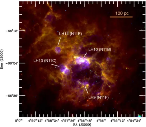
1986). It exhibits several prominent secondary HIIregions along its periphery as well as dense filamentary ISM structures, as traced by the prominent dust and CO emission. It is characterized by an evacuated central cavity with an inner diameter of 170 pc. Four star clusters are the main sources of the ionization in the complex (see Lucke & Hodge1970or Bica et al.2008for studies of the stellar as-sociations in the whole LMC). These clusters are indicated in Fig.1. The rich OB association LH9 is located at the centre of the cavity. The age of this cluster was estimated to be∼7 Myr (Mokiem et al.
2007). The star cluster LH10 (∼3 Myr old; Mokiem et al.2007), is located in the north-east region of the cavity and is embedded in the N11B nebula. The OB association LH13 and its corresponding neb-ula (N11C) are located on the eastern edge of the superbubble. The main exciting source of N11C is the compact star cluster Sk-66◦41 (<5 Myr old; Heydari-Malayeri et al.2000). Finally, the OB asso-ciation LH14 (in N11E) is located in the north-eastern filament. Its
main exciting source is the Sk-66◦43 star cluster. The region also harbours a few massive stars (see Heydari-Malayeri, Niemela & Testor1987, for a detail on its stellar content). The cluster ages and the initial mass functions of the OB associations suggest a sequen-tial star formation in N11, with a star formation in the peripheral molecular clouds triggered by the central LH9 association (Rosado et al.1996; Hatano et al.2006, among others). N11 is also associ-ated with a giant molecular complex. Israel et al. (2003) and Herrera et al. (2013) have suggested that N11 is a shell compounded of dis-crete CO clouds (rather than bright clouds bathing in continuous intercloud CO emission) and estimate that more than 50 per cent of the CO emission resides in discrete molecular clumps.
To construct our local IR-to-submm SEDs in N11, we use data from theSpitzer Space Telescope (Werner et al. 2004) and the Herschel Space Observatory(Pilbratt et al.2010). We complement the submm coverage with observations obtained on the LABOCA instrument at 870µm.
2.2 SpitzerIRAC and MIPS
The LMC has been observed withSpitzer as part of the SAGE project (Surveying the Agents of a Galaxy’s Evolution; Meixner et al.2006) and theSpitzerIRAC (InfraRed Array Camera; Fazio et al.2004) and MIPS (Multiband Imaging Photometer; Rieke et al.
2004) and data have been reduced by the SAGE consortium. IRAC observed at 3.6, 4.5, 5.8, and 8µm [full width at half-maximum (FWHM) of its point spread function (PSF)<2 arcsec ]. The cal-ibration errors of IRAC maps are 2 per cent (Reach et al.2005). MIPS observed at 24, 70 and 160µm (PSF FWHMs of 6, 18 and 40 arcsec, respectively). The MIPS 160µm map of N11 is not used in the following analysis because of its lower resolution (40 arcsec) than to Photodetector Array Camera and Spectrometer (PACS) 160
µm but the data is used for the calibration of theHerschel/PACS 160
µm map (see Section 2.4). The respective calibration errors in the MIPS 24 and 70µm observations are 4 and 5 per cent (Engelbracht et al.2007; Gordon et al.2007). We refer to Meixner et al. (2006) for a detailed description of the various steps of the data reduction. Additional steps have been added to the SAGE MIPS data reduction pipeline by Gordon et al. (2014, see Section 2.5).
2.3 Herschel PACS and SPIRE
The LMC has been observed withHerschelas part of the successor project of SAGE, HERITAGE (HERschel Inventory of The Agents of Galaxy’s Evolution; Meixner et al.2010,2013). TheHerschel PACS (Poglitsch et al.2010) and SPIRE (Spectral and Photometric Imaging Receiver; Griffin et al.2010) data have been reduced by the HERITAGE consortium. The LMC was mapped at 100 and 160µm with PACS (PSF FWHMs of∼7.7 and∼12 arcsec, respectively) and 250, 350 and 500µm with SPIRE (PSF FWHMs of 18, 25 and 36 arcsec, respectively). The SPIRE 500µm map possesses the lowest resolution (FWHM: 36 arcsec) of the IR-to-submm data set. Details of theHerscheldata reduction can be found in Meixner et al. (2013). We particularly refer the reader to the Section 3.9 that describes the cross-calibration applied between the two PACS maps and theIRAS100µm (Schwering1989) and the MIPS 160
µm maps (Meixner et al.2006) in order to correct for the drifting baseline of the PACS bolometers. The PACS instrument has an absolute uncertainty of∼5 per cent (the accuracy is mostly limited by the uncertainty of the celestial standard models used to derive the absolute calibration; Balog et al.2014) to which we linearly add an additional 5 per cent to account for uncertainties in the total beam
area. The SPIRE instrument has an absolute calibration uncertainty of 5 per cent to which we linearly add an additional 4 per cent to account for the uncertainty in the total beam area (Griffin et al.
2013). Additional steps have been added to the HERITAGE PACS and SPIRE data reduction pipelines by Gordon et al. (2014, see Section 2.5).
2.4 LABOCA observations and data reduction
LABOCA is a submm bolometer array installed on the APEX (At-acama Pathfinder EXperiment) telescope in North Chile. Its un-dersampled field of view is 11.4 arcmin and its PSF FWHM is 19.5 arcsec, thus a resolution equivalent to that of the SPIRE 250
µm instrument onboardHerschel. N11 was observed at 870µm with LABOCA in 2008 December and 2009 April, July and September (Program ID: O-081.F-9329A-2008 – PI: Hony). A raster of spiral patterns was used to obtain a regularly sampled map. Data are re-duced withBOA(BOlometer Array Analysis Software).1Every scan is reduced individually. They are first calibrated using the observa-tions of planets (Mars, Uranus, Venus, Jupiter and Neptune) as well as secondary calibrators (PMNJ0450−8100, PMNJ0210−5101, PMNJ0303−6211, PKS0537−441, PKS0506−61, CW-Leo, Ca-rina, V883-ORI, N2071IR and VY-CMa). Zenith opacities are ob-tained using a linear combination of the opacity determined via skydips and that computed from the precipitable water vapour.2We also remove dead or noisy channels, subtract the correlated noise induced by the coupling of amplifier boxes and cables of the detec-tors. Stationary points and data taken at fast scanning velocity or above an acceleration threshold are removed from the time-ordered data stream. Our reduction procedure then includes steps of median noise removal, baseline correction (order 1) and despiking. The re-duced scans are then combined into a final map inBOA. As noticed in Galametz et al. (2013), the steps of median noise removal or baseline correction are responsible for the oversubtraction of faint extended emission around the bright structures. In order to recover (most of) this extended emission we apply an additional iterative process to the data treatment. We use the reduced map as a ‘source model’ and isolate pixels above a given signal-to-noise (S/N). This source model is masked or subtracted from the time-ordered data stream before the median noise removal, baseline correction or despik-ing steps of the followdespik-ing iteration, then added back in. We repeat the process until the process converges.3Final rms and S/N maps are then generated. The average rms across the field is∼8.4 mJy beam−1. Fig.2shows the final LABOCA map. We can see that our iterative data reduction helps us to significantly recover and resolve low surface brightnesses around the main structure of the complex.
2.5 Preparation of the IR/submm data for the analysis
We use the SAGE and HERITAGE MIPS, PACS and SPIRE maps of the LMC reprocessed by Gordon et al. (2014) in the following analysis. They include an additional step of foreground subtraction in order to remove the contamination by Milky Way (MW) cirrus
1http://www.apex-telescope.org/bolometer/laboca/boa/
2The tabulated sky opacities for our observations can be retrieved at http://www.apex-telescope.org/bolometer/laboca/calibration/.
Figure 2. The IR/submm emission of the N11 star-forming complex from 8 to 870µm (original resolution). The colour bars indicate the intensity scale in MJy sr−1. Square root scaling has been applied in order to enhance the fainter structures.
dust. The morphology of the MW dust contamination has been pre-dicted using the integrated velocity HIgas map along the LMC line of sight and using the Desert, Boulanger & Puget (1990) model to convert the HIcolumn density into expected contamination in the PACS and SPIRE bands. The image background is also estimated using a surface polynomial interpolation of the external regions of the LMC and subtracted from each image. All the maps are con-volved to the resolution of SPIRE 500µm (FWHM: 36 arcsec) using the convolution kernels developed by Aniano et al. (2011).4 We refer to Gordon et al. (2014) for further details on these
addi-4Available athttp://www.astro.princeton.edu/∼ganiano/Kernels.html.
tional steps. We convolve the IRAC and LABOCA maps using the same convolution kernel library. For these maps, we estimate the background from each image by masking the emission linked with the complex, fitting the distribution of the remaining pixels with a Gaussian and using the peak value as a background estimate. Pixels of the final maps are 14 arcsec, which corresponds to 3.4 pc at the distance of the LMC.
2.6 Qualitative description of the dust emission
Table 1. Spearman rank correlation coefficients between the IR/submm luminosities from 8 to 870µm (logνLν).
Band 8µm 24µm 70µm 100µm 160µm 250µm 350µm 500µm
24µm 0.85
70µm 0.86 0.93
100µm 0.93 0.93 0.96
160µm 0.96 0.87 0.90 0.96
250µm 0.97 0.85 0.86 0.94 0.97
350µm 0.95 0.83 0.82 0.91 0.96 1.00
500µm 0.94 0.81 0.80 0.89 0.94 0.99 1.00
870µm 0.73 0.68 0.63 0.69 0.73 0.77 0.78 0.79
is primarily coming from polycyclic aromatic hydrocarbons (PAH). PAHs are large organic molecules thought to be responsible of the broad emission features often detected in the near-IR (NIR) to mid-IR (Mmid-IR) bands. They are present everywhere across the complex. The 24µm emission is a tracer of the hottest dust populations. Primarily associated with HIIregions, it is often used (by itself or combined with other tracers) as a calibrator of the star formation rate (SFR; Calzetti2007) in nearby objects. We observe that the MIPS 24
µm emission is more compact than that at longer wavelengths and peaks in the HIIregions of the N11 complex. The MIPS 70µm band is essential to properly constrain the Wien side of the far-IR (FIR) SEDs and traces the warm dust in the complex. Part of the 70µm emission could also be associated with a very small grain (VSG) population. Studies at 70µm in the LMC have indeed revealed a population of VSG (<10 nm; so larger than PAH molecules) probably produced through erosion processes of larger grains in the diffuse medium (Lisenfeld et al.2001; Bernard et al.2008). Erosion processes in magellanic-type galaxies has also been discussed in Galliano et al. (2003,2005). The emission above 100µm is mostly produced by a mixture of equilibrium big (>25 nm) silicate and carbonaceous grains (see Draine & Li2001, among others). The PACS 100 and 160µm observations are associated with the cool to warm dust reservoirs (20–40 K) in the complex: the observations enable us to sample the peak of the dust thermal emission across the field. Residual stripping can be observed in these maps. The SPIRE 250 to 500µm observations are associated with the coldest dust emission (<20 K): they will help us constrain the local dust masses as well as investigate potential emissivity variations of the dust grains in N11.
Using theSpitzer,Herscheland LABOCA maps convolved to a common 36 arcsec resolution (Section 2.4), we calculate the Spear-man rank correlation coefficients between the various bands (log scale) for ISM elements that fulfil a 2σ detection criterion in the Herschelbands. Those coefficients are tabulated in Table 1and highlight the high correlation between the various wavelengths. Correlation coefficients between the 8µm map and bands long-wards of 8µm are similar when the 8µm map is first corrected from stellar continuum (same to the second decimal place). The 8
µm is more strongly correlated with the emission of cold dust traced by the SPIRE bands than with the tracers of hot and warm dust. This could be due to the fact that PAHs (that the 8µm emission mostly traces) are emitted at the surface of the molecular clouds where the shielded dust remains cold. The surface of a cloud (PAH emission) and its interior (cold dust emission) are expected to be probed by the same beam at the spatial scale on which we perform our anal-ysis (10 pc). Emission from PAHs traced by the 8µm emission is less tightly correlated with star-forming regions traced by hot dust tracers such as 24µm for instance (as shown by Calzetti et al.2007, among others). The LABOCA emission at 870µm is as strongly
correlated with the cold dust tracers as with the PAH emission. The correlation between the LABOCA emission and the other bands improves when we restrict the analysis to elements that fulfil a 10σ detection criterion. This indicates that the lower correlation with the LABOCA emission at 870µm is mostly linked with missing diffuse emission across the 870µm map.
3 D U S T S E D M O D E L L I N G O F T H E N 1 1 C O M P L E X
3.1 The method
We select the Galliano et al. (2011) ‘AC model’ in order to interpret the dust SED in each resolved element of the N11 structure.
The SED modelling uses the optical properties of amorphous carbon (Zubko, Krełowski & Wegner1996) in lieu of the proper-ties of graphite, which are more commonly employed to represent the carbonaceous component of the interstellar dust grains. This is motivated by two recent results. First, studies of the dust emission in the LMC by Meixner et al. (2010) and Galliano et al. (2011) have shown that standard grains often lead to GDRs inconsistent with the elemental abundances, suggesting that LMC dust grains have a different (larger) intrinsic submm opacity compared to mod-els which assume graphitic properties for the carbonaceous grains. Analysis byPlanck(Planck Collaboration XXIX2014) have also recently showed that the extinction derived from a modeling of the dust using commonly-used SED fitting techniques (Draine & Li
old stellar mass parameter is only introduced in this analysis in order to estimate the stellar contribution to the MIR bands. The model provides estimates of the fraction of PAHs to the total dust mass ratio. Since the ionized PAH-to-neutral PAH ratio (fPAH+) is poorly constrained by the broad-band fluxes, we choose to fix this value to 0.5; we will discuss the caveats of this approximation in Section 4.3.2.
The free parameters of our model are thus:
(i) the total mass of dust (Mdust), (ii) the PAH-to-dust mass ratio (fPAH), (iii) the index of the intensity distribution (α), (iv) the minimum heating intensity (Umin), (v) the range of starlight intensities (U), (vi) the mass of old stars (Moldstars).
We apply the model to theSpitzer+Herscheldata set (3.6–500µm) and convolve it with the instrumental spectral responses of the dif-ferent cameras in order to derive the expected photometry. The fit is performed using a Levenberg–Marquardt least-squares procedure and uncertainties on flux measurements are taken into account to weight the data during the fitting (1/uncertainty2weighting). The Galliano et al. (2011) model can help us to quantify the total IR luminosities (LTIR) across the region. The model also predicts flux densities at longer wavelengths than the SPIRE 500µm constraint. We will, in particular, use predictions at 870µm in order to decom-pose the observed 870µm emission into its various (thermal dust and non-dust) components in Section 4.5.
Modified blackbodies (MBB) models are commonly used in the literature to obtain average dust temperatures. In order to relate the temperatures derived using this method with the radiation field in-tensity derived from the more complex Galliano et al. (2011) fitting procedure, we fit the 24-to-500µm data using a two-temperature model, i.e. of the form:Lν=Awarmλ−2Bν(λ,Twarm)+Acλ−βcold
Bν(λ,Tcold). In this equation,Bν is the Planck function,Twarmand Tcoldare the temperature of the warm and cold components,βcold is the emissivity index of the cold dust component andAwarmand Acoldare scaling coefficients. We follow the standard approxima-tion of the opacity in the Li & Draine (2001) dust models for the warm dust component (emissivity index of the warm dust fixed to 2). We fix the emissivity index of the cold componentβcoldto the average value derived for the LMC in Planck Collaboration XVII (2011), i.e. 1.5. Fixingβallows us to minimize the degeneracies between the dust temperature and the emissivity index linked with the mathematical form of the model we use and limit the biases resulting from this degeneracy (Shetty et al.2009; Galametz et al.
2012). Potential variations in the grain emissivity across the N11 complex (so using a freeβcold) are discussed in Section 5.3.4.
3.2 Deriving the parameter maps and median local SEDs
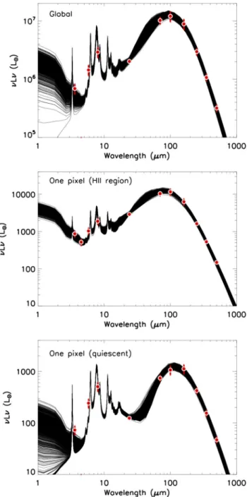
We run the SED fitting procedures for elements with a 2σ detec-tion in all theHerschelbands. We apply a Monte Carlo technique to generate for every ISM element 30 local SEDs by randomly varying the fluxes within their error bars with a normal distribution around the nominal value. A significant part of the uncertainties in SPIRE bands is correlated. To be conservative in the parameters we derive, especially on the dust mass estimates directly affected by variations in the SPIRE fluxes, we decide to link the variations of the three SPIRE measurements consistently during the Monte Carlo procedure. Fig.3shows an example of Monte Carlo realizations of the Galliano et al. (2011) ‘AC’ modelling procedure in three cases: if we consider the N11 complex as one single ISM element (top),
Figure 3. The global SED and two local SEDs (from one ISM element in N11B and one element from the more quiescent ISM) modelled with the Galliano et al. (2011) ‘AC’ model. The various lines show the different realizations of the Monte Carlo technique we use to determine the parameter uncertainties (1000 realizations for each of these three cases).Herschel
measurements are overlaid in red.
for one ISM element in N11B (middle) and for a more quiescent ISM element (bottom). We finally use these various local Monte Carlo realizations to create a median map for each parameter and a median SED for each 14 arcsec×14 arcsec ISM elements. The standard deviations are also providing the uncertainties on each of the parameter derived from the modelling. The parameter maps are discussed in Section 4.
3.3 Residuals from the Galliano et al (2011) fitting procedure
procedure ati=8, 24, 70, 100, 160, 250, 350 and 500µm. In order to obtain a synthetic photometry [Lmodelled
ν (i)] to which observed fluxes
[Lobserved
ν (i)] can be compared directly, we integrate the median
modelled SEDs obtained on local scales in each instrumental filter. Recall that all these observed fluxes are included as constraints in the fitting process. The relative residualsridetermined in this study are defined as
ri= Lobserved
ν (i)−Lmodelledi (i) Lobserved
ν (i)
. (1)
Fig.4(top) compares the spatial distribution of the relative resid-uals ofr8, r24, r70, r100, r160, r250, r350 and r500 across the N11 complex while Fig.4(bottom) shows these residuals as a function of the respective flux densities. Relative residuals are quite small. Except for the 160µm band, the median values are close to 0, so consistent with a reliable fitting of the observational constraints. The lowest residuals appear in the 24µm and the three SPIRE (250, 350 and 500µm) bands, with standard deviations lower than 0.03. The 70-µm residual map shows that our modelling proce-dure slightly underestimates the 70-µm observed flux in the diffuse regions of N11. This could be linked with emission from VSGs pro-duced through processes of erosion of larger grains in the diffuse medium where they are less shielded from the interstellar radiation fields (Bot et al.2004; Bernard et al.2008; Paradis et al.2009). Residuals in the 100µm band seem to be dependent on the ISM element surface brightness (overestimation at low surface bright-nesses, underestimation at high surface brightnesses).
The largest residuals are observed in the PACS 160µm band, with an underestimation of the observed fluxes by 16 per cent throughout the complex. A non-negligible fraction of these residuals could originate from the strong [CII] line emission at 157µm emitting near the peak of the PACS 160-µm filter sensitivity. [CII] emission is indeed detected in every LMC region mapped with PACS. We estimate that a CII-to-TIR ratio of 2–3 per cent would be sufficient to explain most of the residual we observe at 160µm. This ratio is high but consistent with the values estimated in the N11 complex by Israel & Maloney (2011).
Part of the discrepancies at 100 and 160µm could finally be due to a combination of both observational and modelling effects. First, calibration uncertainties in the PACS maps at low surface bright-nesses as well as uncertainties in background/foreground estimates have a significant impact on the fluxes in the most diffuse regions. We remind the reader that 160µm is where the Galactic cirrus peaks while the LMC SED seems to be flatter than that of the MW in the submm regime. We also remind that the modelling procedure we are using assumes AC, thus have a fixed slope of∼1.7 while the Planck Collaboration XVII (2011) results lead to effective emis-sivities closer to∼1.5 on average for the LMC. The residuals we observe could thus also be a sign of different optical properties.
4 T H E D U S T P R O P E RT I E S I N N 1 1
In this section, we examine local IR-to-submm SEDs across the complex. We also analyse the distributions of the modelling pa-rameters derived from the two SED modelling procedures and their correlations. For the rest of the paper, observed maps and parameter maps will be displayed using two different colour tables.
4.1 Local SED variations
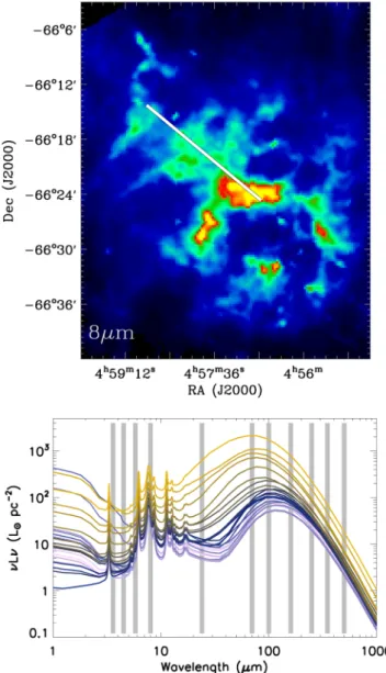
Fig.5(bottom panel) gathers a collection of local IR-to-submm SEDs across the N11 region. These SEDs are extracted from ISM
elements located along the eastern filament down to the north-ern edge of the N11 ring (the location of the selected elements is indicated with a white line in the top panel of Fig.5). We can see how the local SED varies from star-forming regions to more quies-cent regions. Bright star-forming regions (in yellow) show a wider range of temperatures (broader SED) and a lower PAH fraction (weaker features at 8µm) while more quiescent regions (in pur-ple) show colder temperatures and a much narrower range of dust temperatures.
From our local modelling of the IR SEDs, we can derive a map of the IR luminosityLIR. We integrate the models (in aν–fνspace) from 8 to 1100µm. The stellar contribution to the NIR emission was estimated during the SED modelling process. Even if minor in that wavelength range, this contribution is removed from the totalLIRto only take the emission from dust grains into account. Fig.6 (bottom-left panel) shows theLIRmap (in units of L). We can observe that the distribution ofLIRis much more extended than the regions where high-mass star formation is taking place, with a significant contribu-tion arising from more quiescent regions (regions of weaker 24µm emission). This extended distribution is due to the fact that part of the dust emission is not directly related to star formation occurring in the same beam. A fraction of the dust heating is in fact related to the older stellar populations or to ionizing photons leaking out the HIIregions due to the porous ISM in N11 (see Lebouteiller et al.
2012).
4.2 Radiation field and dust temperatures
Fig. 6(upper-middle panel) shows the average cold temperature maps obtained using the MBB model. Temperatures vary signifi-cantly across the N11 complex and range from 32.5 K in the N11B nebula (associated with the LH10 stellar cluster) down to 17.7 K in the diffuse ISM (with a median of 20.5 K for regions detected at a 2 but not 3σ level). The median temperature of the modelled regions is 21.5±2.1 K. This value is similar to that derived if we keep the emissivity indexβfree in the modelling (21.4±3.4 K). For comparison, Herrera et al. (2013) estimated a mean temperature of ∼20 K in the region of N11 from the LMC temperature map of Planck Collaboration XVII (2011), close to what we obtain. The N11 region is representative of the average dust temperatures found in the LMC (Bernard et al.2008). A comparison between N11 and the N158–N159–N160 star-forming complex previously studied by Galametz et al. (2013) shows that N11 is colder on average (median temperature of 26.9 K for the N159 region). The coldest tempera-tures in the N159 complex were estimated in the N159 South region (∼22 K), a significant reservoir of dust and molecular gas but with no ongoing massive star formation detected. The temperatures of the cold dust grains in the diffuse ISM in N11 are similar to those in N159 South. We finally note that the temperature of N11 when considered as one single ISM element (Fig.3top) is 23.1±1.1 K (at the higher end of the uncertainties of the median derived lo-cally). This highlights again that determining the dust temperatures on local scales is essential to constrain the coldest phases of the dust.
Figure 4. Top – distribution of the relative residualsr8,r24,r70,r100,r160,r250,r350andr500to the Galliano et al. (2011) fitting procedure across the N11 complex. The relative residuals are defined as (observed flux−modelled flux) / (observed flux). A residual of 0.2 thus indicates that the model underestimates the observed luminosity by 20 per cent. Bottom – relative residuals to the Galliano et al. (2011) fitting procedure as a function of the respective observed fluxes
Figure 5. Top: the N11 complex observed in the 8µm band. The image has been convolved to the working resolution of 36 arcsec. The white line indi-cates the locations of the ISM elements whose individual SEDs are plotted in the figure below. Bottom: local SEDs across the N11 complex. Colours indicate the position along the above white line, from light purple in the dif-fuse ISM (north-east) to yellow in the bright star-forming region N11B. The vertical grey lines indicate the position of theSpitzerandHerschelbands. normalized to those of the solar neighbourhood (withU=1 cor-responding to an intensity of 2.2×10⁻⁵W m−2). The dust tem-perature of the cold grains (derived from the MBB modelling) and the mean radiation field intensityUthat heat those grains (derived from the ‘AC model’) have very similar distribution, as expected.5 While we analyse the local and median values of these two pa-rameters in this section, their correlation is studied in more details in Section 4.4. The median intensityUof the N11 complex is 2.3 (2.8 if we restrict the median calculation to regions with a 3σ detection in theHerschelbands). Peaks in theUdistribution are observed along the N11 shell, in particular in the N11B nebula
5Uis integrated over the whole range of radiation field intensity, and thus includes the contribution from hot regions. The temperatureTcderived from the MBB modelling is not constrained byλ <100, and thus does not include the hot phases.
where it reaches a maximum of 31.8 times the solar neighbourhood value. This value is similar to that estimated in the LMC/N158 re-gion in Galametz et al. (2013). N158 is an HIIregion where two OB associations were detected (Lucke & Hodge1970). In N158, the southern association hosts two young stellar populations of 2 and 3–6 Myr (Testor & Niemela 1998). These cluster ages are close to those expected from the intermediate-mass Herbig Ae/Be population detected in the N11B nebula by Barb´a et al. (2003). The two regions are thus very similar in terms of evolutionary stage.
4.3 The dust distribution
4.3.1 Total dust masses
Fig.6(bottom-middle panel) shows the surface density mapdust (units of Mpc−2) obtained with the ‘AC model’. The dust distribu-tion appears to be very structured and clumpy, with major reservoirs in N11B as well as in the N11C nebula located on the eastern rim. Secondary dust clumps are located along the N11 shell. The median of the dust surface density across N11 is 0.22 Mpc−2. The total dust mass derived for the complex is 3.3±0.6×10⁴M
. Un-certainties are the direct sum of the individual unUn-certainties derived from our Monte Carlo realizations. The main peaks in the dust dis-tribution coincide with the molecular clouds catalogued by Herrera et al. (2013, identification on the SEST CO(2–1) observations at a 23 arcsec resolution) as shown later in Fig.9(bottom panel). We find that only 10 per cent of the total dust mass (∼2.7±0.5× 10³M
) resides in these individual clumps.
Using the same data set than this analysis and a single temperature blackbody modified by a broken power-law emissivity (BEMBB), Gordon et al. (2014) produced a dust mass map of the whole LMC. They obtain a total dust mass that is a factor of 4–5 lower than values derived from standard dust models like the Draine & Li (2007) models. We convolve ourdustmass map to their 56-arcsec working resolution to position our dust estimates (for the same area) in that dust mass range. We find that the mass estimated for the whole N11 region in Gordon et al. (2014) is 2.5 times lower than the dust mass we derive (on average 2.4 times lower fordust< 0.2 M pc−2 and 2.6 times lower for
dust > 0.2 M pc−2). The dust masses we estimate with the ‘AC model’ are moreover 2.5 times lower than those obtained if we use standard graphite in lieu of amorphous carbon to model the carbonaceous grains (as already shown in Galliano et al.2011and Galametz et al.2013). Our dust masses thus reside in between those derived by the BEMBB model and a standard ‘graphite’ dust model. These results highlight how the choice of dust composition can dramatically influence the derived dust masses.
Finally, many studies have shown that total dust masses are usually underestimated when derived globally rather than locally (Galliano et al. 2011; Galametz et al. 2012, among others). On global scales, the SED modelling technique is poorly disentangling between warm / cold / very cold dust at submm wavelengths – due to the combined effects of a poor spatial resolution and a small num-ber of submm constraints – and the coldest phases of dust can be diluted in warmer regions. This ‘resolution effect’ is not a physical effect but a methodological bias linked with the non-linearity of the SED modelling procedures. To test this effect in N11, we model the complex as a single ISM element. We obtain a total dust mass of 2.8×10⁴M
Figure 6. Maps of the parameters derived from our two SED modelling techniques. The 24µm map (convolved to a resolution of 36 arcsec) is shown for reference in the upper-left panel (square root scaling). Top-middle panel: cold dust temperature in kelvins. Top-right panel: mean starlight heating intensity, with
U=1 corresponding to the intensity of the solar neighbourhood (log scale). Bottom-left panel: FIR luminosity in Lpc−2(log scale). Bottom-middle panel: dust surface density in Mpc−2. All the parameter maps are obtained using the Galliano et al. (2011) modelling technique (with the choice of amorphous carbon grains to model the carbon dust) except the cold dust temperature map that is obtained using the two-temperature MBB fitting technique. Bottom right panel: PAH fraction to the total dust mass (in per cent).
4.3.2 PAH fraction to the total dust mass
PAHs are planar molecules (∼1 nm) made of aromatic cycles of car-bon and hydrogen and are thought to be responsible for the strong emission features observed in the NIR to MIR (Leger & Puget
1984). The main features are centred at 3.3, 6.2, 7.7, 8.6 and 11.3
µm. Draine & Li (2007) and Zubko, Dwek & Arendt (2004, bare silicate and graphite grain models) found that 4.6 per cent of the total dust mass in the MW could reside in PAHs. UsingSpitzer/IRS spectra, Compi`egne et al. (2011) obtain a largerfPAH(7.7 per cent) for the same environment. It has been shown that the PAH fraction also varies significantly depending on the intensity of the radiation field and with the metallicity of the environment (Engelbracht et al.
2008; Galliano, Dwek & Chanial2008, among others). Our fitting procedure can help us assess these variations on local scales. Fig.
6(bottom-right panel) shows the distribution of the PAH-to-total dust mass fraction (in per cent) across the N11 complex. We find
a medianfPAHacross the complex of ∼4 per cent, thus close to the Draine & Li (2007) and the Zubko et al. (2004) studies.6 How-ever, the fraction varies significantly across the complex. Lower fractions (<1 per cent) are for instance estimated for regions with high radiation field intensities while higher fractions (>6–12 per cent) are observed in more diffuse regions of the complex. This is similar to what has been observed in the LMC N158–N159–N160 complex (Galametz et al.2013) and consistent with the expected destruction of PAH molecules through photodissociation processes scaled with the radiation field hardness and intensity (Madden
2005).
Caveats –laboratory experiments have shown that the various PAH bending modes (C–C, C–H etc.) vary with the PAH charge:
6A lower value of f
Figure 7. Correlation plots between various model parameters: the dust temperature (Temp) in K, the mean starlight heating intensity normalized to the intensity of the solar neighbourhood (U), the PAH-to-total dust mass in percent (fPAH), the IR luminosity in L(LIR) and the dust surface density in M pc−2(dust). All parameters are obtained using the Galliano et al. (2011) modelling technique except the cold dust temperature that is obtained using the two-temperature MBB fitting technique. The Spearman rank correlation coefficients are added to each plot. The ISM elements are coloured as a function of their MIPS 24-µm surface brightness. The inset plot shows the 24-µm surface brightness histogram and provides the colour scale for the plots (from yellow for higher 24-µm surface brightnesses to light purple for lower 24-µm surface brightnesses). The grey curve on the top panel indicates the best-fitting curve. The equation is provided in the panel. The dashed grey curve indicates the fit with a coefficient fixed to 5.7 (U =(T/18.6)5.7).
neutral PAHs preferably emit around 11µm while ionized PAHs preferably emit around 8µm. Because of our lack of constraint in the MIR spectrum, we fixed the fraction of ionized PAHsfPAH+ to 0.5. This means that (i) thefPAHwe derive naturally scales, by model construction, with 8µm-to-LIRluminosity ratio (correlation coefficientr=0.91) and (ii) the neutral PAHs scale with the ionized PAHs. Yet, by studying localfPAHin the Small Magellanic Cloud [SMC; 12+log(O/H)∼8.0; Kurt & Dufour1998, Sandstrom et al. (2012) find that PAHs in the SMC tend to be smaller and more neu-tral than in more metal-rich environments. This could also be the case in the LMC, affecting the PAH mass. MIR spectra would be necessary to properly quantify the ionized-to-neutral PAH fraction in N11. On a side note, Jones et al. (2013; see also Jones2014) recently proposed nanometer-sized aromatic hydrogenated amor-phous carbon grains (a-C(:H)) in lieu of free flying PAHs to explain the MIR diffuse interstellar bands we observe in the Galaxy. A more systematic comparison of the two hypotheses would enable us to test their ability to reproduce the observations of different environments.
4.4 Correlations between parameters
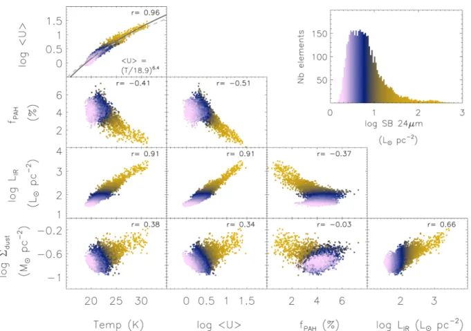
Fig. 7 presents correlation plots between the dust temperature (Temp), the mean starlight heating intensity (U), the PAH fraction
fPAH, the IR luminosityLIRand the dust surface densitydust. We are using ISM elements of 14 arcsec, which means that our neigh-bouring pixels are not independent. However, a quick test using 42 arcsec pixels shows that the correlations observed in Fig.7are not affected by our choice of pixel size.
The top-left panel shows the strong relation between the dust temperature and the mean starlight heating intensity across the N11 complex. In thermal equilibrium conditions, the energy absorbed by a dust grain is equal to that re-emitted. This leads to a direct link between the temperature of the grainT, its emissivityβand the intensity of the surrounding radiation fieldU, withU∝T(4+β). By model construction, the submm effective emissivity of our ‘AC model’ isβ=1.7 (see Galliano et al.2011), soUis proportional to T5.7. We fit our ISM elements, fixingβ to 1.7, and derive the relationU =(T/18.6±0.02)5.7, thus a normalizing equilibrium dust temperature of 18.6K (dashed line in Fig.7, top panel). Fitting our ISM elements with no a priori onβleads to the relation:U = (T/18.9±0.05)6.4±0.10
elements modelled. This discrepancy is driven by ISM elements with logU<0.5, i.e. the ‘diffuse’ ISM of N11. These elements show a very steep submm slope. They reach effectiveβhigher than 2 when you letβvary, values that are difficult to explain from our current knowledge about grain physics. Because we fixβto 1.5 in our MBB fitting technique, our cold temperatures are higher than what would be derived with a higher index (i.e.β=1.7 or more). This translates into an increase of the fitting coefficient from 5.7 to 6.4.
Fig.7also shows the close relation betweenfPAHandU.fPAH reaches a constant fraction (∼4 per cent) whenUis lower than ∼3. Above this threshold value, we observe a linear decrease offPAH with logU. The lower panels in Fig.7also show the correlations withdust. We do not observe strong variations of column density across the complex. Most of the variations of the IR power are rather driven by the variations in the radiation field intensity. Dense regions have a higherUand a lowerfPAH, as expected from regions with embedded star formation.
4.5 Dissecting the components of the 870µm emission
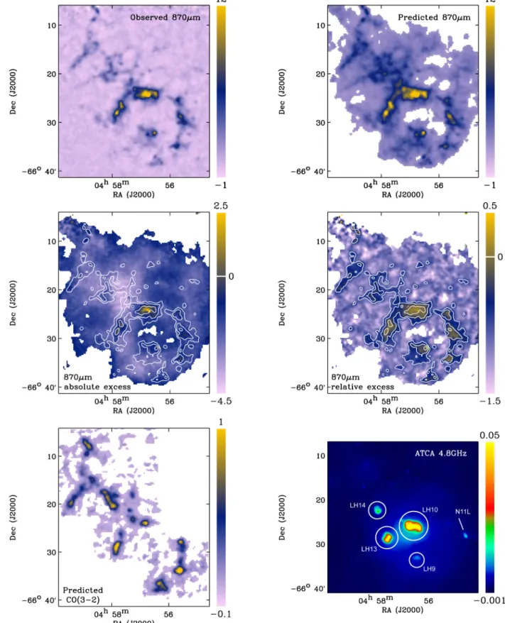
As explained in Section 2.3, the data reduction of LABOCA data can lead to a filtering of faint extended emission. If our iterative data reduction procedure helps recover a significant amount of emis-sion around the brighter structures, part of the very extended faint emission (well traced by the Herschel/SPIRE instrument for in-stance) is not recovered. Only the flux densities in regions with sufficient S/N (i.e.>1.5) can then be trusted. For these reasons, we decide not to include the 870µm data as a direct constraint in the dust modelling procedure. However, the LABOCA 870µm map traces the coldest phases of dust in the complex. By com-paring the 870µm emission predicted by our dust models (fixed emissivity properties) with the observed 870µm emission, it can also help us investigate potential variations in the grain emissivity in the submm regime. We decompose the various contributors to the 870 µm emission in this dedicated section. Part of the emis-sion at 870 µm in this particularly massive star-forming region is linked with non-dust contributions, namely12CO(3–2) emission line falling in the wide LABOCA passband (at 345GHz) and ther-mal bremsstrahlung emission produced by free electrons in the ionized gas. We will quantify how much of the measured
870-µm surface brightness can reasonably be attributed to thermal dust emission, free–free continuum and CO(3–2). This study will allow us to investigate the presence (or not) of any submm emission not explained by these ‘standard’ components (the so-called ‘submm excess’).
4.5.1 Thermal dust emission at 870µm and excess maps
From our local SED modelling (the physically motivated ‘AC model’), we derive a prediction of the pure thermal contribution to the 870µm observations. The observed and predicted maps at 870µm are shown in Fig.8(top panels). Their resolution is our working resolution of 36 arcsec. To compare the two maps, we compute the absolute differences between observations and model predictions defined as (observed flux at 870µm−modelled flux at 870µm) and the relative differences between observations and model predictions defined as (observed flux at 870µm−modelled flux at 870µm) / (modelled flux at 870µm). The maps (that we call the absolute and relative excess maps) are shown in Fig.8(middle
panels). We overlay the contours of LABOCA S/N to highlight re-gions where the LABOCA emission is higher than a 1.5σthreshold. The image shows that most of the structures below our S/N thresh-old correspond to regions where the SED model overpredicts the observed 870µm (negative difference). As previously suggested, part of the diffuse emission might be filtered out during the data reduction in these faint regions. In regions above our S/N criterion, the distribution of the relative excess seems to follow the structure of the complex. The observed emission at 870µm is close to the predicted value (weak emission in excess) on average and the rela-tive excess reaches∼20 per cent at most in the centre of N11B. We will now try to quantify the non-dust contribution to the 870µm flux that could partly account for this excess.
4.5.2 CO(3–2) line contribution
A12CO(1–0) mapping of LMC giant molecular clouds (GMCs) has been performed using the Australia Telescope National Facil-ity Mopra Telescope as part of the Magellanic Mopra Assessment (MAGMA;745 arcsec resolution) project (Wong et al.2011). We are using these observations to estimate the12CO(3–2) line contri-bution to the 870µm flux. To do the conversion, we need to assume a brightness temperature ratioR3-2, 1−0. In LMC GMCs, this ratio ranges between 0.3 and 1.4 (average of the clumps: 0.7), with high values (>1.0) being associated with strong Hαfluxes (Minamidani et al.2008). They find an average brightness temperature ratio of about 0.9 in the N159 star-forming complex. The dust temperature in N11 being lower than that in N159 as shown in Section 4.2, the R3-2, 1−0 is probably lower than this value. We used the average R3-2, 1−0ratio of 0.7 derived in Minamidani et al. (2008) to convert the CO(1–0) map into a CO(3–2) map. We use the formula from Drabek et al. (2012) to convert our CO line intensities (K km s−1) to pseudo-continuum fluxes (mJy beam−1):
C
(mJy beam−1)(K km s−1)−1= 2kν3
c3
gν(line)
gνdν B,
(2)
wherekis the Boltzmann constant,ν is the frequency, Bis the telescope beam area,gν(line) is the transmission at the frequency of the CO(3–2) line and gν dν is the transmission integrated
across the full frequency range.gν(345GHz)/gνdνis∼0.017 for
LABOCA (Siringo, private communication; ESO/MPIfR; 2007). The derived CO(3–2) map is shown in Fig.8(bottom left). We convolve the 870µm map to the resolution of the CO(3–2) map (Gaussian kernel) to compare the two maps. We estimate a con-tribution of∼15–20 per cent in LH13,<6 per cent in LH10 and LH9 and from 4 to 12 per cent in the west ring and in the northern elongated structure detected by LABOCA. We note that LH14 is not fully covered in the public MAGMA map we are using. These values are reported in Table2.
4.5.3 Free–free contribution
Fig.1shows the Hα distribution (whose distribution should be co-spatial with that of the free–free component across the com-plex) while Fig.8(bottom right) presents a mosaicked image of the 4.8-GHz radio continuum emission taken with the Australia Telescope Compact Array (ATCA). The radio (ATCA) maps at
Figure 8. Top left: 870-µm flux density in MJy sr−1observed with LABOCA (resolution of SPIRE 500µm, i.e. 36 arcsec). Top right: 870-µm flux density in MJy sr−1predicted by the AC model, i.e. pure thermal dust emission (same resolution). Middle left: 870-µm absolute excess in MJy sr−1defined as (observed
Table 2. IR-to-submm photometry of the OB associations in N11 and non-dust contribution to the 870µm fluxes.
LH9/N11F LH10/N11B LH13/N11C LH14/N11E
Centrea (RA) 04h56m35s 04h56m48s 04h57m46s 04h58m12s
(Dec.) −66◦3204 −66◦2418 −66◦2736 −66◦2138
Radius (arcsec) 100 200 150 120
8µm (Jy) 2.7±0.3 14.9±1.5 7.2±0.7 3.2±0.3
24µm (Jy) 7.5±0.7 84.2±8.4 28.0±2.8 7.7±0.8
70µm (Jy) 101.4±10.1 815.6±81.6 312.1±31.2 110.2±11.0
100µm (Jy) 153.6±15.4 1220.3±122.0 507.0±50.7 190.8±19.1
160µm (Jy) 162.8±6.5 968.4±38.7 456.0±18.2 193.8±7.8
250µm (Jy) 76.9±5.4 416.7±29.2 212.6±14.9 102.4±7.2
350µm (Jy) 38.1±3.8 191.4±19.1 102.5±10.3 50.5±5.1
500µm (Jy) 16.1±1.6 77.1±7.7 42.3±4.2 21.3±2.1
870µmb (Jy) 4.2±0.3 12.2±0.9 7.1±0.5 3.1±0.2
f870,free-free (per cent) 7.4 10.4 9.1 6.3
f870, CO (per cent) <6 <4 <20 –
Notes.aThe photometric apertures are shown in Fig.8(bottom-right panel).bObserved flux density not corrected for the non-dust contribution.
4.8 and 8.6 GHz (resolution of 33 and 20 arcsec, respectively) ob-tained from Dickel et al. (2005) are used to model the free–free emission where radio emission is detected. We first convolve the two maps to the working resolution of 36 arcsec using a Gaussian kernel. We then estimate the 870-µm, 6.25 and 3.5-cm flux densities in the four OB associations of the complex (LH9, LH10, LH13 and LH14) shown in Fig.8(middle). The circles indicate the positions and sizes of the photometric apertures. The 8–870-µm flux densi-ties in the four individual regions are provided in Table2. We use the two ATCA constraints to extrapolate the free–free emission in the 870µm band, assuming that the free–free flux density is pro-portional toν−0.1. We estimate free–free contributions of 10.4, 9.1, 7.4 and 6.3 per cent in LH10, LH13, LH9 and LH14, respectively. These values are reported in Table2.
Potential synchrotron contamination –in this analysis, we assume that the radio emission across the complex is dominated by free– free emission. However, radio continuum observations can trace both thermal emission from HIIregions and synchrotron emission. Polarized synchrotron emission can, for instance, be produced in supernova remnants (SNRs). This is the case in particular for the SNR N11L detected in the ATCA observations and indicated in Fig.8. This SNR is however located outside the regions where the 870µm excess peaks. Synchrotron radiation can also be an arti-ficial source of X-rays in the ISM. Using X-ray observations of the N11 superbubble from the Suzaku observatory, Maddox et al. (2009) detected non-thermal X-ray emission around the OB as-sociation LH9. However, the photon index of the required non-thermal power-law component is too hard to be explained by a synchrotron origin. Our hypothesis of negligible contamination of the 870µm emission in N11 by synchrotron emission thus seems reasonable.
4.5.4 Conclusions
The excess above the pure thermal dust emission we observe in Section 4.5.1 is weak and can be, within uncertainties, ac-counted for by the various non-dust contributions (CO line emis-sion and free–free emisemis-sion) we estimated. We conclude that the 870 µm can fully be reproduced by these three standard components.
5 C O M PA R I S O N B E T W E E N T H E D U S T A N D T H E G A S T R AC E R S
In this section, we use the dust surface density map we gener-ate to study the relation between the dust reservoir and the gas tracers. We use H I and CO observations to derive an atomic and a molecular surface density map of N11. By studying the variations of the ‘observed’ GDR across the complex, we will be able to explore the influence of each of the assumptions we made.
5.1 The gas reservoirs in N11
5.1.1 Atomic gas
Figure 9. Relation between dust and gas in N11. Top left: HImap of N11. Top right:dustmap of the complex (units of Mpc−2) with HIcontours overlaid. The levels are 3×10²¹, 4×10²¹and 5×10²¹atoms cm−2(from thinner to thicker lines). The dashed circle indicates the location of the supergiant shell located north to the N11 star-forming region. Bottom left: MAGMA CO map of N11. Bottom right:dustmap of N11 with a MAGMA CO contour at 1.4 K km s−1(the survey has a 3σsensitivity limit of 1.2 K km s−1). Molecular clouds identified by Herrera et al. (2013) are shown in red. Additional molecular clouds previously identified by Israel et al. (2003) are overlaid in cyan. Both studies have identified molecular clouds based on SEST observations of N11. The radii of the circles indicate the geometrical radii of the clouds fitted to the SEST observations at these positions.
5.1.2 Molecular gas
The CO(1–0) line emission is widely used as an indirect tracer of the H2abundance. The 1.4 K km s−1contour of the MAGMA CO(1–0) map presented previously in the paper is overlaid on the dustmap in Fig.9(bottom). Israel et al. (2003) also mapped some of the N11 clouds in12CO(1–0) and12CO(2–1) emission lines as part of the ESO-SEST key programme (FWHM=45 and 23 arcsec, respectively). Herrera et al. (2013) present a follow-up study using fully sampled maps. Both studies provide catalogues of the phys-ical properties of individual molecular clouds (overlaid in Fig.9) across the N11 complex. We observe that N11 is composed of many individual molecular clumps that account for a significant part of
Choice of theXCO factor – in order to build a map of the H2 column density, we need to convert the intensities of the MAGMA CO(1–0) map into masses. The ‘standard’XCOfactor in the solar neighbourhood is∼2×1020 cm−2(K km s−1)−1(Scoville et al.
1987; Solomon et al.1987) but has a strong dependence on the ISM physical conditions, especially with metallicity (Bolatto et al.
2013). Because of the lower dust content in low-metallicity objects, the UV photons penetrate deeper into the molecular clouds, leading to a drop in the optical depth and a photodissociation of the CO molecule (so less CO emission to trace the same H2mass). The XCOfactor is thus usually higher in low-metallicity environments. Indirectly using dust measurements to trace the gas reservoirs, Leroy et al. (2011) derived anXCOfactor of 3×1020cm−2(K km s−1)−1 for the LMC.XCOfactors were also estimated from the NANTEN survey of nearly 300 GMCs over the whole LMC (Fukui et al.1999; Mizuno et al.2001). They find an average value of∼9×1020cm−2 (K km s−1)−1. The estimate was then refined to be 7×1020cm−2(K km s−1)−1by improving the rms noise level by a factor of 2 (Fukui et al.2008). By targeting more specifically the CO clumps of N11, XCOwas estimated to be∼5×1020cm−2(K km s−1)−1in Israel et al. (2003) and∼8.8×10²⁰α−1
vir in Herrera et al. (2013), withαvirthe virial parameter corresponding to the ratio of total kinetic energy to gravitational energy. In their analysis, Herrera et al. (2013) suggest to useαvir ∼2 [this leads to aXCOfactor of 4.4×1020 cm−2(K km s−1)−1]. In our analysis, we decide to use the statistically robust average from the whole MAGMA GMC sample obtained by Hughes et al. (2010), i.e. 4.7×1020cm−2(K km s−1)−1. This assumes that αvir=1. We will call this value the MAGMAXCOfactor. We note that in the case of anαvirequal to 2, theXCOvalue will be close to the GalacticXCO(4.7 / 2=2.35). As a comparison, we will thus also present the results obtained when a standard GalacticXCO factor is used. We discuss the consequences of these choices further in Section 5.3.1.
5.1.3 Surface density maps of the gas
The MAGMA CO map at a 1 arcmin resolution (that of the HI map) is already provided on the MAGMA web site. We regrid this map and the HI map to a final pixel grid of half the resolution of the HImap, i.e. 7 pc at the distance of the LMC. We derive the HIsurface density map (HI) and the H2surface density map
(H2) by dividing the local H I masses (MHI) and the local H2
masses (MH2) by the area of our reference pixel (final units: M pc−2). We multiply the
HI map by 1.36 to take the presence of
helium into account. The MAGMAXCOfactor being derived from virial masses, ourH2 map includes all the material contributing to the dynamical mass of the cloud, thus already includes helium (this contribution is added however in the GalacticXCOcase). The two final maps will be, respectively, referred to as the atomic and molecular gas surface density mapsatomicandmol, CO, their sum as gas. Assuming that the region follows the Kennicutt (1998) relation [SFR=2.5×10⁻⁴(gas)1.4], we can use thegasmap to derive local estimates of the SFRs. For the regions detected at a 2σ level in theHerschelbands, the SFR ranges from 4.5×10⁻³to 2.4× 10⁻¹M
kpc−2yr−1, with an average
SFR of 4.4×10⁻²M kpc−2yr−1across the whole complex. Using YSO candidates in the N11 region, Carlson et al. (2012) estimated the SFR in the region to be between 1.8 and 8.8×10⁻²M
kpc−2yr−1(depending on the time-scale selected for the Stage I formation, i.e. for embedded sources). The value we estimate from the gas mass is consistent with that SFR range.
5.2 Relations between dust and gas surface densities
We convolve thedustmap (resolution: 36 arcsec) to the resolution of thegasmap using Gaussian kernels (same pixel grid). We then derive an ‘observed’ total GDR map of N11. The map obtained
Figure 11. Dust surface density as a function of the total gas surface density. The molecular mass is estimated using anXCOfactor of 4.7×1020cm−2(K km s−1)−1on the left-hand panel and a GalacticX
COfactor of 2.0×1020cm−2(K km s−1)−1on the right-hand panel. On both plots, black points are ISM elements where MAGMA CO data is available and grey points where MAGMA CO data is not available. The larger squares overlaid over the individual ISM elements indicate the averageddustper bins ofgas(we choose regular bins in logarithmic scale). The linear fit to the pixel-by-pixel relation (in the shape of
gas=GDR×dust) is indicated for the whole sample with the black solid line, for ISM elements withdust<0.2 Mpc−2with the dotted line and for ISM elements withdust>0.2 Mpc−2with the dashed line.
using the MAGMAXCOfactor to derive the molecular gas is shown in Fig.10. The corresponding probability distribution is shown in the right-hand panel. The vertical line indicates the Galactic GDR value derived by Zubko et al. (2004, i.e. 158). The inset compares this distribution with that restricted to the regions covered by the MAGMA public release. The range ofgaswe are probing covers about an order of magnitude. The distribution of GDR broadly fol-lows the dust distribution, with highest values of the GDR observed in the most diffuse regions and lowest values detected towards the HIIregions. HIdominates the local gas masses in many regions of the complex.
Fig.11shows the relation between the dust surface density and the atomic+molecular gas surface density (MAGMAXCOcase on the left-hand panel and GalacticXCOcase on the right-hand panel). Black points distinguish ISM elements where MAGMA CO data is available in the publicly released map. They represent about 45 per cent of our ISM elements. Grey points indicate elements for which the CO information is not available. They are identical in both panels. Some of these ‘grey’ elements might have CO emission (but are simply not covered). This is probably the case for regions that possess a non-negligible dust surface density at the top of the ‘grey cloud’ of points. Additional molecular gas would shift these elements and tighten the relation betweendust and gas. The larger squares indicate the averageddustper bins ofgas(we choose regular bins in logarithmic scale). The error bars indicate the scatter within thesegasbins. In thedustrange we are studying here (0.1≤dust≤0.5 Mpc−2), the relation betweendustand gasseems to be linear. In the case of the MAGMAXCOfactor, we observe a flattening of the relation abovegas=60 Mpc−2. The flattening resides within the error bars in the GalacticXCOcase.
We take the uncertainties on the individualdust into account to derive the linear scaling coefficients linking the dust surface densities to the gas surface densities (so to derive the error-weighted averaged GDR of the sample). The thick line in the plots of Fig.11
indicates these relations. We see that the GDR of the whole region is close to 180 in bothXCO cases. How does this compare to the expected GDR in the LMC [12+log(O/H)=8.3–8.4; see Russell &
Dopita1990? We can predict this value using the formula of R´emy-Ruyer et al. (2014) for a broken power-law and anXCO,Zcase (i.e.
XCO∼Z−2). This leads to a GDR of 350, thus∼50 per cent more than the global ratio we find. To probe the variations of GDR with the dust surface density, we cut ourdust range in two intervals, estimating the GDR fordust <0.2 M pc−2(dotted line) and dust>0.2 Mpc−2(dashed line). The values are 186±12 and 140±33, respectively, in the case of MAGMAXCOand 184±12 and 140±30, respectively, in the case of a GalacticXCO). The GDR thus decreases with the dust surface densities in the N11 complex. This decrease was previously observed in a strip of the LMC in Galliano et al. (2011) or in the recent study of Roman-Duval et al. (2014).
5.3 Discussion on the low ‘observed’ GDR
Our analysis of GDR in N11 leads to values lower than those ex-pected for an environment such as the LMC. We recall that several assumptions have been made to derive this ‘observed’ GDR map: we assume that (i) theXCOfactor is constant across the complex, (ii) the CO traces the full molecular gas reservoir, (iii) the HIline is optically thin in the region and (iv) the dust composition does not vary across the complex. In the following section, we discuss the impact of these hypotheses on the derived GDR and analyse the possible origin of its decrease with the dust surface density.
5.3.1 Underestimation or variations in theXCOfactor
Figure 12. Local variations of theXCOfactor estimated using a constant GDR=350 across the complex. Units are in cm−2 (K km s−1)−1 (log scale). We limit the study to ISM elements above the 3σsensitivity limit of the MAGMA CO(1–0) map.
arising from the multiple OB associations in N11, theXCOfactor could be above the mean MAGMA value that is driven by less en-ergetic environments. Israel (1997) for instance suggests anXCO factor of 6×1020cm−2(K km s−1)−1in the north-east filament of N11 and of up to 2.1×1021 cm−2(K km s−1)−1in the N11 ring itself.
Let us assume a constant GDR of 350 across the region. Which conversion factors would then be required to reach this value?XCO would be equal to (350×dust−HI)/ICO. Fig.12shows the map
of theXCOfactors we obtain. Because low S/N pixels around the edge of the CO-bright clouds are very dependent on the baselines and the signal identification method used to generate the MAGMA CO map, we choose to limit this study to regions above the 3σ sensitivity limit of the MAGMA survey. We observe the highestXCO values near the bright OB associations LH10 and LH13 and in the north-eastern filament. The derivedXCOfactor can vary by an order of magnitude: it ranges between 5.2×1020cm−2(K km s−1)−1and 4.9×1021cm−2(K km s−1)−1, with a mean value of 1.3×1021cm−2 (K km s−1)−1. The minimum factor we obtain is consistent with our nominal (MAGMA) choice forXCObut using a higherXCOfactor would indeed increase the local GDR values towards the expected LMC GDR in most of these regions. The maximumXCOfactor we find is twice the value estimated for the ring by Israel (1997). Even if possible, these very highXCOfactors are, nevertheless, expected in more extreme environments than the LMC, such as the dwarf irregular galaxies NGC 6822 or the SMC (Leroy et al. 2011). A modification of theXCOfactor alone is probably not sufficient to fully explain the low ‘observed’ GDR.
5.3.2 CO-dark gas
Studies tracing gas through the dust emission or the gamma rays emission (produced through cosmic ray collisions in the Galaxy; see Grenier, Casandjian & Terrier2005; Ackermann et al.2012) have highlighted the presence of H2that is not detectable through CO observations. This molecular phase, called the ‘CO-dark’ phase is particularly difficult to quantify and cannot be related to the
CO-emitting reservoirs through the usualXCO factor. If we consider that this ‘missing molecular phase’ is responsible for the low GDR observed in N11, we can quantify its abundance by doingdarkgas= 350×dust−HI−mol, CO, withdarkgasthe surface density of the molecular dark gas not traced by CO. Before continuing with this analysis, we need to take into account the fact that in the more quiescent regions of the complex, part of the missing gas mass could be already linked with our lack of CO constraints due to the limited coverage of the public MAGMA map. If we assume a constant GDR of 350 throughout the complex,∼8.6×10⁵M
are missing from the total gas budget in the regions with no CO data (see Fig.8bottom left). We use the good correlation betweendust andmol, COin the regions covered in CO (Spearman coefficient r=0.5 anddust =0.16±0.007mol0.19,±CO0.02) to estimate the CO-emitting molecular gas in the regions not covered in CO. Using this completedmol, COmap, we can then derive the mass of the dark gas in the region. We find a fraction of the dark gas to the total gas mass equal to 55–60 per cent. The fraction of the dark gas to the total molecular mass (fDG=Mdarkgas/(Mdarkgas+Mmol, CO)) is equal to 70–80 per cent, with larger values outside the dust peaks of N11. By theoretically modelling the dark component, Wolfire, Hollenbach & McKee (2010) predict thatfDGwould be relatively invariant with the incident UV radiation field strength (∼0.3 in the Galaxy for instance) but that this value could increase with (i) a decreasing visual extinction and (ii) a decreasing metallicity. If our results are consistent with these trends, the very highfDG fraction we obtain is pushing the models to the limits. This suggests that a hidden reservoir of CO-dark gas is probably not the unique explanation to the low ‘observed’ GDR throughout N11.
We note that further observations would be needed to correctly estimate the CO-faint phase in the complex. The CO-dark reservoirs could also be quantified using the [CII] 157µm line as suggested by Madden et al. (1997). Several studies have indeed shown that the [CII] emission is more extended than that of CO (Israel & Maloney
2011; Lebouteiller et al.2012).
5.3.3 Optically thick HI
The HIcolumn densityNHIcan be estimated from the measured HI
brightness temperatureTBand the optical depthτ using equation 3-38 from Spitzer (1978):
NHI=1.823×10
18
TB τ
1−e−τdv, (3)
whereTBis the measured brightness temperature (K),τis the optical depth andvis the velocity. In this analysis, we assume that the 21 cm line is optically thin across the complex in order to derive the local HImasses. This reduces the equation toNHI,thin=1.82×10¹⁸
TBτ dv. However, because the HIoptical depth strongly depends onNHI, the assumption of optically thin HIstarts to be questionable
for large column densities. Recent studies have proposed optically thick HIenvelope around CO clouds to explain the large scatter in the relation between the HI velocity integrated intensity and the submm dust optical depth (see Fukui et al.2014, 2015, for instance). In their study of the Perseus molecular cloud, Lee et al. (2012,2015) estimated the optical depth effects to be responsible of an underestimation of the HImass by a factor of 1.2–2. Using equation (3-37) from Spitzer (1978) and a single spin temperature ofTs=60 K, we estimate that we would need an HIcolumn density of about 1020cm−2per km s−1to reachτ=1. If we consider an HI line width of∼14 km s−1(mean value of the H