T
AXATION OFM
ULTI-P
RODUCTF
IRMS WITHC
OSTC
OMPLEMENTARITIESArlynn Quinton White, III
A dissertation submitted to the faculty of the University of North Carolina at Chapel Hill in par-tial fulfillment of the requirements for the degree of Doctor of Philosophy in the Department of
Economics.
Chapel Hill 2020
Approved by: Jonathan Williams David Agrawal Gary Biglaiser Brian McManus
c
2020
Arlynn Quinton White, III ALL RIGHTS RESERVED
ABSTRACT
ARLYNN QUINTON WHITE, III: Taxation of Multi-Product Firms with Cost Complementarities.
(Under the direction of Jonathan Williams)
ACKNOWLEDGMENTS
Completing this project has been the singular intellectual achievement of my life and would not have been possible without the support of many generous people.
First, thank you to my advisor, Jon Williams, for teaching me something every time we met, continuously advocating for me, and somehow always letting me dive deeply into an idea without sinking. I will forever be grateful for your support and friendship.
A special thanks to each of my committee members, David Agrawal, Gary Biglaiser, Brian McManus, and Juan Carlos Su´arez Serrato, for providing me the technical skills to do sophisticated analysis without losing sight of the intuition which makes it fun. You always had faith I was making progress despite the detours and occasional long silences. I always felt my well-being was as valued as my scholarship and that has made all the difference.
The support from UNC economics extends well beyond those formally tasked with keeping me on track. Thank you to my fellow graduate students Adam Haas, Andrew Hanson, Gonzalo Asis, Dave Leather, Zach Mozenter, Brad Shrago, Eddie Watkins, Aisling Winston, and Yi Zhong for conversations, some economic – most not, when I needed help (or a break). Thank you to the many faculty members who provided insightful guidance and caring support, especially Simon Alder, Jane Cooley Fruehwirth, Luca Flabbi, Donna Gilleskie, Qing Gong, Peter Hansen, Fei Li, Luca Maini, Peter Norman, Can Tian, Valentin Verdier, Kyle Woodward, and Andy Yates. Also, a sincere thank you to the staff of UNC economics, especially Natasha Gilliam and Cindy Wunder, for calmly dealing with my frantic emails and help navigating bureaucratic challenges.
Thank you to my parents, Quint and Susan White, for truly unconditional love, instilling in me a deep desire to continue learning, and a value for education.
Finally, thank you to my wife and best friend, Lane, for constant love, support, and never once pointing out you got a doctorate in literally half the time. Also, a special thanks to Albert and Denny for substantially raising the opportunity cost of staying at the office.
TABLE OF CONTENTS
LIST OF TABLES . . . vii
LIST OF FIGURES . . . viii
1 Taxation in the Aviation Industry: Insights and Challenges . . . 1
1.1 Introduction . . . 1
1.2 Overview of Aviation Taxation . . . 2
1.3 Effect of Taxation on Fares . . . 8
1.4 Implications and Justifications for Over-Shifting . . . 12
1.4.1 Market Factors Influencing Tax Incidence . . . 13
1.4.2 Network Impact . . . 14
1.5 Conclusion . . . 15
2 Taxation of Multi-Product Firms with Cost Complementarities . . . 16
2.1 Introduction . . . 16
2.2 Data . . . 20
2.2.1 Sample Selection . . . 21
2.2.2 Variables . . . 22
2.2.3 Aviation Taxation . . . 24
2.2.4 Aviation Industry . . . 27
2.3 Empirical Model of Demand and Oligopoly Firms . . . 30
2.3.1 Demand . . . 31
2.3.3 Pricing Equilibrium . . . 35
2.4 Estimation . . . 36
2.4.1 Instruments . . . 38
2.5 Results . . . 42
2.6 Tax Simulation and Counterfactuals . . . 45
2.6.1 Solving for Optimal Prices . . . 46
2.6.2 Tax Simulations . . . 46
2.6.3 Counterfactuals . . . 49
2.7 Conclusion . . . 56
A Appendix . . . 59
A.1 Appendix . . . 59
A.1.1 Simple model . . . 59
A.1.2 Estimation . . . 63
A.1.3 Notation . . . 66
REFERENCES . . . 71
LIST OF TABLES
1.1 Aviation Tax Reforms . . . 3
1.2 Results . . . 11
2.1 Variable Description and Sources . . . 23
2.2 Summary Statistics . . . 23
2.3 Summary of Aviation Taxation: 1993 to 2015 . . . 25
2.4 Demand Parameters . . . 43
2.5 Marginal Cost Parameters . . . 44
2.6 Counterfactual Policy Comparison . . . 51
LIST OF FIGURES
1.1 Total Tax Rates . . . 4
1.2 U.S. Ticket Tax Rate . . . 6
1.3 Breakdown of PFCs by Charge Level . . . 7
2.1 Routes and Markets . . . 22
2.2 Tax Share of Fares . . . 25
2.3 Specific Taxes . . . 26
2.4 Mean Fares and Total Passenger Volume . . . 28
2.5 Percentage of Nonstop Passengers . . . 28
2.6 Mean Route Distance . . . 29
2.7 Routes and Carriers per market . . . 30
2.8 PFC Implementation . . . 42
2.9 Segment Marginal Cost and Quantity . . . 45
2.10 Distribution of Direct and Indirect Incidence . . . 48
2.11 Centrality and Incidence . . . 49
2.12 Indirect Incidence and Airport Centrality . . . 50
2.13 Consumer Surplus and Hub Subsidy: Declining Revenue . . . 53
2.14 Consumer Surplus and Hub Subsidy: Revenue-Neutral . . . 54
2.15 Distribution of Fare Changes . . . 55
2.16 Heterogeneity in Carrier Response . . . 56
A.1 Network Structure . . . 59
CHAPTER 1
TAXATION IN THE AVIATION INDUSTRY: INSIGHTS AND CHALLENGES
1.1 Introduction
Taxation influences a wide range of behavior. For example, taxes in the aviation industry may affect a passenger’s fare, the size of the aircraft a carrier operates on a route, and the number of departures from an airport. Understanding the influence of taxes on passengers, carriers, or airports is valuable in ensuring government finances are raised efficiently without placing undue burden on participants. Aviation taxes are substantial. The mean effective tax rate, defined as the total taxes and fees divided by the passenger fare, was approximately 15% in 2015.
Furthermore, how the government raises and dispenses funding has changed dramatically in the aviation industry over the last 25 years. Despite this change, relatively little research studies the extent of taxation or analyzes its influence on economic variables such as the price. This paper makes two contributions to fill this void in the literature. The first portion describes how aviation taxation in the United States has evolved since the early 1990’s. The second portion develops an empirical model that exploits variation in the level of taxes across similar routes and over time to estimate how equilibrium fares change in response to taxes. Initial results suggest taxes are over-shifted to consumers (i.e., a $1 increase in taxes results in more than a $1 increase in the tax-inclusive fare for the consumer). The paper then discusses potential explanations for this result: the nature of competition in the industry and the propagation of taxes within a network.
Studying taxation in the aviation industry is difficult because the primary data set on fares contain only total fares without any decomposition into the base fare, taxes or fees. Despite this difficulty, several studies have documented the roles of taxes in the aviation industry. In a 1997
Transportation Research Record article, Heimlich provides a history of the U.S. Ticket Tax, ar-guing the regulation of the industry in its formative years and airline travel’s characterization as a luxury good influenced the level of taxation (Heimlich 1997). In a 2004 article, Karlsson, Odoni, and Yamanaka provide a cross-sectional description of domestic airline tickets for the second quar-ter of 2002 and find an effective tax rate of approximately 15.5% (Karlsson et al. 2004). Garrow, Hotle, and Mumbower describes how the recent trend of unbundling fares has the potential to im-pact revenue given the domestic tax structure (Garrow et al. 2012). More recently, Agrawal, White, and Williams write a tax calculator that identifies the precise taxes paid on a given itinerary to doc-ument spatial and temporal variation in the industry (Agrawal et al. 2018b). Prior to this paper and their study, no research had comprehensively tracked taxes in the industry over a prolonged period. International aviation markets are also taxed quite substantially and have a similarly sparse litera-ture. In a recent paper, Bradley and Feldman examine the influence of international taxes on the airline industry (Bradley and Feldman 2018). However, they focus on the salience of taxes and not the effect of major tax rate reforms over time. They find taxes are largely passed through but not over-shifted to passengers. Comparing empirical estimates of pass-through between international and domestic markets is difficult due to differences in the demand elasticity, supply elasticity, and other market characteristics. In the subsequent sections, this paper contributes to the literature by studying the effect of taxes on fares.
1.2 Overview of Aviation Taxation
To summarize aviation taxation and interpret the empirical analysis in the following section, one must define terminology specific to the aviation industry. A market is defined by the ordered pair of its origin and destination airports as well as by its round-trip status. Thus, for cities A and B, four potential markets are A to B round-trip, A to B one-way, B to A round-trip, and B to A one-way. Within a market, a route is defined as the path or ordered set of airports used in traveling from an origin to a destination, as well as the return for round-trip markets. Thus, two passengers with the same origin and destination but different connecting airports are flying two different routes within the same market. Throughout the paper, the word “tax” is used to generically cover both taxes and government fees added to a ticket.
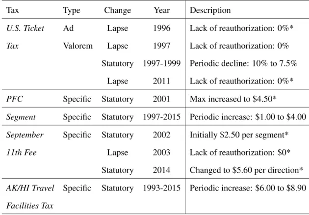
In 1993, carriers were responsible for collecting two taxes on domestic flights in the continental U.S., both still collected today. First, the U.S. Ticket Tax is a percentage-based tax added to a base fare. Second, a Passenger Facility Charge (PFC) is a dollar amount added to a base fare for enplanements at a subset of airports that levy them. Subsequently, the U.S. ticket tax rate changed, dramatically at times, per-segment taxes were added, various exceptions for rural routes were added and eliminated, and new fees such as the September 11th Security fee were added and modified. Table 1.1 summarizes the set of taxes and fees and how they have changed since 1993.
Table 1.1: Aviation Tax Reforms
Tax Type Change Year Description
U.S. Ticket Ad Lapse 1996 Lack of reauthorization: 0%*
Tax Valorem Lapse 1997 Lack of reauthorization: 0%
Statutory 1997-1999 Periodic decline: 10% to 7.5%
Lapse 2011 Lack of reauthorization: 0%*
PFC Specific Statutory 2001 Max increased to $4.50*
Segment Specific Statutory 1997-2015 Periodic increase: $1.00 to $4.00
September Specific Statutory 2002 Initially $2.50 per segment*
11th Fee Lapse 2003 Lack of reauthorization: $0* Statutory 2014 Changed to $5.60 per direction*
AK/HI Travel Facilities Tax
Specific Statutory 1993-2015 Periodic increase: $6.00 to $8.90
Note: *indicates vertical bar in Figure 1.1
in the given year-quarter. Aside from the lapse of the U.S. Ticket Tax during 1996 and 1997, discussed in greater detail below, the mean effective tax rate has remained between 10 and 15% but can be higher or lower for a particular route. Taxes not related to air travel, such as corporate income taxes or taxes on jet fuel, are not included in these figures or in our analysis.
Figure 1.1: Total Tax Rates
While the mean rate of all routes has remained relatively stable, taxation on individual routes varies considerably. For example, even excluding the lapses in 1996 and 1997, taxes on a round-trip ticket from Memphis (MEM) to Orlando (MCO) via Atlanta (ATL), ranged from 10.9% to 25.8%. Variation is driven by non-tax-related changes to the base fare, but statutory changes and congressional and Federal Aviation Administration (FAA) authorization to levy certain taxes are also important factors. The vertical bars in the figure indicate notable tax events, summarized in Table 1.1, over the past 25 years. From left to right in Figure 1.1, these events are the lapse of the U.S. Ticket Tax in 1996, the increase in 2001 of the PFC maximum per enplanement to $4.50, the
September 11th Security Fee introduction in 2002 as well as lapse in 2003, the lapse of the U.S. Ticket Tax in 2011, and finally the change in structure of the September 11th Security Fee in 2014. To better explore what drives statutory changes in the tax rates in Figure 1.1, it is instructive to outline how each of the individual taxes in Table 1.1 has changed. The U.S. Ticket Tax (also called U.S. Domestic Transportation Tax or the U.S. Excise Tax) is the only ad valorem tax applied to the base fare. Figure 1.2 shows the tax rate of the U.S. ticket tax from 1993 through 2015 for flights in the continental United States. Figure 1.2 also highlights two notable features of Ticket Tax policy over the last 25 years. In the 1990’s and again in 2011, Congress allowed authorization to collect taxes for the Airport and Airway Trust Fund (AATF) to expire. First, from January 1, 1996, through August 26, 1996, itineraries were not subject to the Ticket Tax. Shortly thereafter, Congress again failed to authorize the AATF from January 1 to March 6 of 1997. Finally, in 2011, authorization again expired from July 23 to August 7. To calculate the tax rate, when taxes are in effect for part of the quarter, we weight by the number of days in the quarter for which the tax was not expired.
The second notable feature of the U.S. Ticket Tax is that routes involving certain designated airports have a reduced rate. As indicated by the dashed lines in Figure 1.2, from the 4th quarter of 1997 to the 4th quarter of 1999, flight segments along a route which involved at least one rural airport were subject to a lower rate. Additionally, but not depicted in the figure, for domestic flights involving Alaska or Hawaii, the tax does not apply to the portion of the flight which occurs over international water or land. In lieu of paying the full U.S. Ticket Tax, flights with one endpoint in Alaska or Hawaii and an origin or destination in the continental United States are required to pay the Alaska and Hawaii Travel Facilities Tax, a specific tax which has gradually increased from $6 in 1993 to $8.90 in 2015 along with a prorated Ticket Tax rate covering the portion of the flight over U.S. territory.
Figure 1.2: U.S. Ticket Tax Rate
fare. It was introduced at a rate of $1 per segment by the Taxpayer Relief Act of 1997 and gradually increased to $4.00 per segment by 2015. One notable feature of the segment tax is flight segments involving rural airports are exempt from the tax.
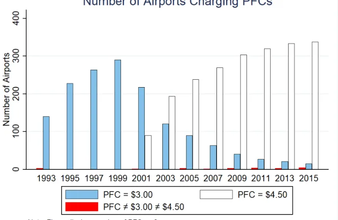
Passenger Facility Charges are airport-specific fees assessed when a passenger enplanes at the designated airport. For an airport to assess the charge, the PFC must be authorized by the FAA. The revenue is treated as local funds and restricted to use on specific long-term capital projects. First introduced in 1992, PFCs initially had a maximum allowable charge of $3.00 per airport. In 2001, the Wendell H. Ford Aviation Investment and Reform Act for the 21st Century increased the maximum charge to $4.50 (the second vertical bar in Figure 1.1). A maximum of two PFCs can be assessed on a one-way trip and four on a round-trip flight. Figure 1.3 displays the number of airports assessing various levels of nonzero PFCs since 1993. The number of airports charging
a PFC has steadily increased over time. By 2015, over 350 airports were charging a PFC, with approximately 95% of them charging the maximum allowable $4.50. Just before the maximum allowable PFC was raised to $4.50 in 2001, many airports charged the then maximum of $3.00, although this was not always the case historically. After the 2nd quarter of 2001, airports steadily sought and received approval to institute or raise the PFC to the new cap.
Figure 1.3: Breakdown of PFCs by Charge Level
this reform, the fee is $5.60 for a one-way trip and $11.20 for a round-trip itinerary, regardless of the number of segments. Given a route, depending on the number of stops and round-trip status, the reform resulted in a slight (60 cents) to moderate ($6.20) increase in the tax burden.
1.3 Effect of Taxation on Fares
The party legally required to remit a tax does not, in general, bear the economic burden of a tax. In perfectly competitive environments, the less elastic party bears a greater burden of the tax; furthermore, the change in the consumer price from a $1 tax increase is bounded between $0 and $1. With constant marginal costs, consumer prices rise by a full dollar. In more complicated settings, however, a tax may be over-shifted to one party (i.e., a $1 increase in taxes results in more than a $1 increase in the price). Over-shifting could be due to market power, products being close complements or substitutes, or cost complementarities between a firm’s products (Weyl and Fabinger 2013; Agrawal and Hoyt 2018). For the aviation industry, specifically, carriers’ market power and cost complementarities from network transactions (i.e. the cost of a flight depending on other related flights) imply a wide range of theoretical possibilities, including over-shifting. These concerns frame the discussion following the results presented here.
Itinerary data are from the Data Bank 1B (DB1B) of the U.S Department of Transportation’s Origin and Destination Survey, a 10% sample of all domestic itineraries in the United States. The sample period ranges from 1993 to 2015 and the data are aggregated so an observation is at the route-carrier-year-quarter level. Because the DB1B does not contain tax data directly, information from federal legislation, the IRS code, federal memorandums and industry documentation dating back to the 1990’s are used to determine the federal taxation on a route in a given quarter. Itinerary fares are decomposed into the base fare set by the carrier and the individual statutory taxes owed at the time of the flight based on the itinerary’s route. For a more detailed description on how the itinerary fares are decomposed and the restrictions placed on the data, see Agrawal et al. (2018b). The natural log of population and income for the origin and destination cities is from the Bureau of Economic Analysis. The remaining control variables are constructed using route characteristics and flight information reported in the DB1B.Number of Carriers is the number of carriers oper-ating in the market. Airport Presenceis the share of routes a carrier serves out of the originating
airport. HHI is the Herfindahl-Hirschman Index (sum of squared market shares) for the market.
LCC in Marketequals 1 if there is a low-cost carrier operating in the market and zero otherwise. Brueckner, Lee, and Singer highlight the influential role low cost carriers play in determining the competitive conditions within a market (Brueckner et al. 2013). MilesandMiles Squared are the number of miles flown along the route.
Routes often have different tax treatments, both relative to other routes within their market and across time as taxes lapse or changes to the law occur. To estimate the influence of taxes on fares, one must control for factors correlated with taxes which influence the fare and restrict comparisons to similar routes with different tax treatments. The baseline model, presented in Equation 1.1, compares fares between routes with the same origin and destination, number of segments, and round-trip designation. Using a panel data fixed effects approach, the average level of a route’s fare in a year-quarter is explained by taxes, a set of controls common to the airline literature, and time, carrier and market-segment fixed effects. By identifying the effect within routes that have the same origin and destination (i.e., market) and number of segments, this specification allows comparisons between routes with similar demands as well as cost considerations. Formally,
F arer,t =ζm,s+ζt+ζc+βT axr,t+Xr,tγ+r,t (1.1)
where the dependent variableF arer,tis the mean fare (i.e., base fare plus taxes) for routerin time
periodt, ζm,s are market fixed effects interacted with indicators for the number of segments and
whether the trip is round-trip,ζtare time fixed effects, andζcare carrier fixed effects. Depending
on the specification, T axr,t captures either the total PFC or the total specific taxes on the route
in period t. The vector Xr,t is the full set of controls outlined below. The model builds on an
extensive literature in economics and transportation research which examines how demand and cost factors correspond to equilibrium fares (Garrow, Jones, and Parker 2007; Brueckner et al. 2013; Mumbower, Garrow, and Newman 2015).
unobservable to the researchers, many factors determining prices cannot be directly controlled for in the regression but are intended to be captured by the model’s fixed effects. For example, the model relies on time fixed effects to capture fuel price changes under the assumption fuel price is set in a national market. This may not be true to the extent, for example, state and local sales and excise taxes cause after-tax prices of fuel to differ across the United States. Time fixed effects also capture macroeconomic shocks over the panel. Changes to the broader economy which impact all routes are captured with the time fixed effect, but market-specific temporal shocks would not be.
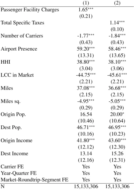
Besides time fixed effects, the model utilizes market fixed effects. These dummy variables capture time-invariant factors common to an origin-destination airport pair such as the non-stop distance between endpoints and expected weather conditions at the endpoints. Because demand-side characteristics and supply-demand-side costs may differ for one-way and round-trip flights and by the number of segments flown, the market fixed effects are interacted with a full set of indicators for the number of segments and round-trip status. These capture cost considerations such as the number of landings and takeoffs. While it may be tempting to narrow the fixed effects to the route level, the identifying assumption is that time-invariant demand and supply-side variables are market rather than route specific. Further, route fixed effects would eliminate all within-market variation and rely exclusively on temporal variation to identify the effect of taxation on fares. Given many taxes are a function of the number of segments, limiting comparisons to those with the same number of segments is prudent, allowing use of some within-market variation while also controlling for costs. Table 1.2 presents the results. The staggered implementation of PFCs at airports across the country provides an intuitive source of variation to initially exploit. The coefficient onPassenger Facility Chargesimplies a $1 increase in the total PFC along a route results in an average increase of $1.65 on the tax-inclusive fare. The coefficients on the control variables each have the expected sign. An additional carrier, especially if a low-cost carrier, is associated with a decline in the fare on average. Higher levels of concentration at either the airport or market level, as captured byAirport PresenceandHHIrespectively, imply higher fares on average. Longer routes are associated with higher fares, although at a declining rate as indicated by the negative coefficient onMiles Squared. It is difficult to know the correct expected sign of the population and income coefficients, as either
could be associated with higher demand or lower cost. Given the controls and fixed effects, all four coefficients are positive, although some are not statistically significant. Relative to a model without controls, the coefficient on Passenger Facility Chargesis stable, suggesting the fixed effects are capturing many factors correlated withPassenger Facility Charges.
Table 1.2: Results
(1) (2)
Passenger Facility Charges 1.65∗∗∗ (0.21)
Total Specific Taxes 1.14∗∗∗
(0.10)
Number of Carriers -1.77∗∗∗ -1.84∗∗∗
(0.43) (0.43)
Airport Presence 59.20∗∗∗ 58.46∗∗∗
(13.31) (13.65)
HHI 38.80∗∗∗ 38.10∗∗∗
(3.04) (3.06)
LCC in Market -44.75∗∗∗ -45.61∗∗∗
(2.21) (2.21)
Miles 37.08∗∗∗ 36.68∗∗∗
(2.15) (2.15)
Miles sq. -4.95∗∗∗ -5.05∗∗∗
(0.29) (0.29)
Origin Pop. 16.54 20.00∗
(10.46) (10.64)
Dest Pop. 46.71∗∗∗ 46.95∗∗∗
(10.16) (10.23)
Origin Income 41.80∗∗∗ 43.60∗∗∗
(12.12) (12.30)
Dest Income 13.14 15.26
(12.16) (12.31)
Carrier FE Yes Yes
Year-Quarter FE Yes Yes
Market-Roundtrip-Segment FE Yes Yes
N 15,133,306 15,133,306
If the implementation of PFCs, even if not federal policy, is correlated with the introduction of other taxes on average, as suggested by Figure 1.3 and Table 1.2, then the over-shifted estimates from column (1) may be erroneously assigning fare changes from all taxes to some PFC changes. In column (2) all the specific taxes and fees present on a route for a year quarter (segment taxes, September 11th fees, Alaska Hawaii ticket tax, and PFCs) are summed together to generateTotal Specific Taxes. This represents our preferred specification. While there is some evidence of over-shifting, the coefficient is reduced substantially in magnitude and not statistically different from full pass-through at a 95% confidence level. However, the estimate is statistically greater than one at lower confidence levels. We can statistically reject that pass-through is less than or equal to one with a p-value of 0.08. Using the point estimate from this regression, a $1 increase in taxes is associated with an approximately $1.14 increase in the tax-inclusive fare. The specification with total specific taxes is especially appealing because carriers may only be concerned with the pass-through of taxes overall, as opposed to the passthrough of individual types of taxes.
1.4 Implications and Justifications for Over-Shifting
While fares increasing by more than a tax seems counterintuitive, the prior economic literature suggests over-shifting is common for many goods (Poterba 1996; Besley and Rosen 1999; Kenkel 2005). This section discusses potential theoretical justifications for this finding which may warrant further research.
Even with over-shifting, the results do not imply profit increases for carriers or that carriers would support tax increases. Higher fares do not imply higher profits because passenger quantities and costs are likely to change as well. The preferred estimate of $1.14 refers to an increase in the passenger fare. Within the increased price, the dollar of tax revenue is not kept by the carrier and, on the margin, the increase in fare above the tax further reduces the quantity demanded. Also, the quantity reduction could cause per-unit costs to rise (e.g. switching to a smaller plane). An increased fare may cause profit per passenger to increase but weakly decreases total profit relative to an untaxed scenario.
Network industries are especially difficult to model, and the policy implications of these re-sults should be interpreted cautiously. First, aviation taxes appear to be largely passed through to
passengers. This would be true even if the estimate of pass-through was merely equal to $1 but not over-shifted. Second, taxes share similar properties with other cost shocks to inputs in production, and those cost shocks may be largely passed through, or even over-shifted, to passengers as well.
Aviation taxation, and the industry in general, is complex. A number of interesting topics such as the relationship between the unbundling of fares and taxes or the precise impact of the U.S. Ticket Tax lapse on carrier profits, while interesting, are outside the scope of this paper. Rather than attempt to draw broader conclusions regarding aviation policy, the results speak to the need to conduct further research and explore potential theoretical justifications, such as market power and network effects, which could cause the tax to be over-shifted.
1.4.1 Market Factors Influencing Tax Incidence
One possible explanation of over-shifting is airlines have market power on routes. Recent theoretical work highlights the complex relationship between competition, demand and supply elasticities, and how changes in equilibrium outcomes affect incidence (Weyl and Fabinger 2013; Delipalla and Keen 1992; Muehlegger and Sweeney 2017). These studies suggest over-shifting may arise with imperfect competition. With imperfect competition, the pass-through of taxes de-pends on whether competitor firms are expected to match the price increase or expected to try to steal market share. Without additional assumptions, it is difficult to explore how market power interacts with the overall result. Simply utilizing a given measure of competition, such asNumber of CarriersorHHI, is unlikely to be sufficient.
it has greater incentive to internalize the impact from changes in fares and pass-through taxes at a lower rate. This effect is enhanced by the disbursement of some aviation taxes, such as PFCs, back to their original point of taxation. Furthermore, effects of competition are likely to have substantial non-linearity. The marginal effect of going from a monopoly to duopoly is likely very different than adding a third or fourth carrier. Even with a long-panel and relatively rich data, the model presented here cannot fully address these effects. Taxes may be passed through at substantially different rates depending on the number of carriers, the price sensitivity of passengers, and the ease of entry in a market. The results presented above likely mask interesting heterogeneity along multiple dimensions of market power which could have rich regulatory and antitrust implications. 1.4.2 Network Impact
Airline networks, rather than simply connecting passengers between an origin and destination, are structured so routes have a greater “density” or quantity of passengers along routes. These “economies of density” are motivated by engineering cost considerations, notably larger planes with a lower cost per passenger mile, and the ability of carriers to route passengers in different markets onto the same plane to maximize cost savings. Many economists attribute the hub-and-spoke structure of the network as the natural outcome of carriers reacting to economies of density (Berry, Carnall, and Spiller 1996; Brueckner and Spiller 1994). Economies of density interact with many economic variables of interest, producing interesting paradoxes for researchers to resolve.
Even a simple theoretical model can provide some intuition for how the role of a network might influence pass-through and cause the estimates above to be over-shifted. Imagine a simple network with three cities: two spoke cities A and B, and a hub H. Passengers can fly directly from A to H or B to H (or vice-versa) but not directly from A to B. Passengers wishing to travel from A to B must connect via H. As a result of economies of density, the more passengers on a flight, then the cheaper the cost, and hence the lower the fare. Now, for simplicity, imagine a tax is assessed only on passengers enplaning at airport A. Passengers flying from A to H, including passengers with final destination B, will pay this tax, but a passenger flying only from H to B would not. The tax will directly dissuade some A to H and A to B passengers from flying, as it raises the fare on those routes. This lowers the number of passengers on both flights A to H and H to B (because
there are fewer A to B passengers). The marginal cost of the flights increases because there are fewer passengers aboard. Because the marginal cost of the H to B flight increases, then all else equal, the fare for passengers flying from H to B will increase as well, despite not being taxed. Thus, cost complementarity between different routes may cause taxes to increase fares on both directly taxed routes as well as other closely connected routes. As prior studies have shown, cost complementarities are likely substantial in the U.S. aviation industry (Berry et al. 1996; Brueckner and Spiller 1994). These arise from larger, more efficient aircraft, using those aircraft at higher load factors, and more intensive use of airport facilities.
Without more information, the empirical model presented above cannot account for the net-work structure or any cost complementarity which arises as a result of that structure. If netnet-work characteristics, whether cost complementarities or another factor, influence how taxes are passed through to passengers, then the model could find over-shifting, because tax changes occurring on related routes may be attributed to the direct tax change occurring on the route.
1.5 Conclusion
CHAPTER 2
TAXATION OF MULTI-PRODUCT FIRMS WITH COST COMPLEMENTARITIES
2.1 Introduction
Understanding the determinants of tax incidence is critical for setting policy to efficiently raise revenue and to minimize distortions from taxation. As Coase (1946) notes, in most market settings, products connected via demand or cost relationships can extend the burden of taxation beyond the taxed product. Despite the theoretical ambiguity surrounding changes in price, cost, and ultimately welfare when a tax is assessed on one product, there is little empirical evidence that quantifies the permeation of tax incidence across related products. Quantifying the intensity of these secondary effects can provide guidance for optimal taxation in these settings, and insight into related issues like antitrust and trade policy. In this paper, I estimate a model of competition in the U.S. aviation industry to measure tax incidence and calculate the impact of counterfactual tax policies in a net-work setting where cost complementarities1between routes and oligopolistic competition can lead to widespread incidence from localized taxes.
The U.S. aviation industry is well-suited to the study of tax incidence and the impact of cross-product relationships on incidence for many reasons. First, taxes are substantial, reaching 15% of the fare under current policy. Second, taxes change frequently during the sample period, 1993 to 2015. They vary spatially, by type (percentage or unit), and the extent to which they favor cer-tain types of products, such as nonstop vs. connecting. This variation is valuable for identifying parameters and assessing the welfare implications of different policy characteristics. Third, cost complementarities between products (i.e., flight itineraries) within a carrier’s network are well doc-umented.2 Finally, the classification of cross-product demand and cost relationships is relatively
1Cost complementaries, or declines in marginal cost from the production of another product, arise due to the hub
and spoke nature of airline’s networks in which passengers share flight segments in route to their final destination.
straightforward. Demand relationships are defined by a route’s origin and final destination. Cost relationships are defined by a shared flight segment common to each route. For example, consider two itineraries. The first originates in Boston, flies to Philadelphia, and has a final destination of Atlanta. The second originates in Boston, flies to Philadelphia, and has a final destination of Detroit. The Boston to Philadelphia segment serves as an input to both itineraries. Cost comple-mentarities arise as the cost of operating a segment such as Boston to Philadelphia declines with more passengers due to the use of larger, more fuel-efficient planes and the lower opportunity cost of selling a seat.
Empirical research on taxation in complex settings is often difficult due to a lack of data. Specifically, to measure tax incidence requires detailed information on prices, quantities, and taxes at a disaggregated level for all products impacted by the tax. Also, adequate exogenous variation in tax rates is necessary to identify its relationship to equilibrium outcomes such as prices and quanti-ties. As in many industries, information on tax rates is not readily available for the airline industry. One contribution of this research project more broadly is to collect information on taxes for the airline industry. I collect information from administrative records (e.g., FAA, Homeland Security, TSA), federal legislation and statutes (e.g., Airport and Airway Revenue Act of 1970, Taxpayer Relief Act of 1997, American Infrastructure Investment and Improvement Act of 2007), and in-dustry guidelines and documentation (e.g., Airlines for America and Aviation Services LLC) for the period of 1993-2015. I use this information to code a tax calculator that decomposes observed fares into a base fare, set by the carrier, and each of the taxes levied on every itinerary (Agrawal et al. 2018b). White, Agrawal, and Williams (2018) use the tax calculator to provide evidence avi-ation taxes may be over-shifted (i.e., a $1 tax results in more than a $1 increase in price). Despite taxes composing a substantial share of fares, prior researchers have not comprehensively studied the effect of taxes due to data availability. I contribute to an extensive literature on the determinants of fares.3 I also demonstrate the utility of taxes as instruments for fares in the aviation industry, a
(1995), Berry, Carnall, and Spiller (2006), and Berry and Jia (2010)
3See Borenstein (1989), Borenstein and Rose (1994), Lederman (2007), Goolsbee and Syverson (2008), Snider
strategy which can be replicated to address a wide range of research questions.
To measure tax incidence across products and simulate counterfactual policies, I develop and estimate a discrete-choice, oligopoly model in which carriers compete by setting fares. Specifi-cally, I consider a theoretical model similar to that of Berry et al. (2006) in which carriers account for their ownership of multiple products within a market and cost complementarities across prod-ucts generated by their observed network structure. Passengers choose the route which offers them the greatest utility conditional on the price and other characteristics of the route. I use parameter estimates from the model to describe how taxes permeate a network and to conduct a series of counterfactual exercises. Consistent with prior theoretical and empirical work on taxation in net-works, cost complementarities increase incidence on taxed products and cause incidence to spill over across a firm’s products. Taxes on more centrally located airports (i.e., hubs) have larger spillover effects and greater negative effects on consumer welfare.
Changes to tax policy can significantly impact consumer welfare. In counterfactual policy simulations, eliminating taxes in a quarter provides a transfer of $1.1 B, or 5.24% of consumer welfare, to consumers. A more relevant exercise is to hold tax revenue constant and estimate the impact on consumers from policy changes. Similar to Fajgelbaum, Morales, Su´arez Serrato, and Zidar (2018), one possibility would be to eliminate spatial distortions in the tax either by setting the same tax on each route, or alternatively the same tax on each segment, while holding total tax revenue constant. Standardizing taxes across routes increases consumer welfare by .2%, while standardizing taxes per segment leaves consumer welfare essentially unchanged. Finally, I estimate the potential welfare benefits from setting taxes which exploit the presence of cost complementar-ities. Relative to a world with standardized segment taxes, I find consumer welfare improves by .08% when the ten most central airports are subsidized. The relatively small change in welfare for revenue-neutral tax policies masks heterogeneity in effects across routes and types of products. The multi-product nature of markets and the cost structure of firms help to limit the welfare cost of taxation. Multiple products or routes allow passengers to find close substitutes, while cost com-plementarities potentially generate savings as passenger substitution lowers costs on alternative routes.
This paper contributes to several strands of research which span public finance and indus-trial organization. Within public finance, the results are important for theoretical models of tax incidence (Delipalla and Keen 1992; Fullerton and Metcalf 2002). Whereas much of the prior theoretical literature often focuses on factors such as the relative magnitude of supply and demand elasticities, the curvature of demand, and the nature of competition (Weyl and Fabinger 2013), my model highlights how cost complementarities potentially influence pass-through and incidence. Hamilton (2008) introduces a model of tax incidence where consumers purchase multiple products from oligopolistic firms in a transaction. I contribute to the literature on empirical estimates of factors of incidence (Poterba 1996; Besley and Rosen 1999; Kenkel 2005; Harding, Leibtag, and Lovenheim 2012; Kleven, Landais, Saez, and Schultz 2014). More generally, I contribute to the literature on the effects of consumption taxes (Kanbur and Keen 1993; Chetty, Looney, and Kroft 2009; Crawford, Keen, and Smith 2011).
Finally, my paper is most closely related to recent empirical work by Houde et al. (2017); Flaaen, Hortac¸su, and Tintelnot (2019); and Agrawal, White, and Williams (2018a) which high-light the interaction between taxes and the multi-product nature of firms and markets. Houde et al. (2017) examine the importance of a firm’s internal cost structure, Amazon’s distribution network, on the incidence of taxes. They utilize growth in the distribution network to infer the relevant trade-offs between increased tax liabilities and reduced shipping costs. Flaaen et al. (2019) ex-amine a set of differentially taxed complementary products, washers and dryers, and the resulting change in prices. Lastly, Agrawal et al. (2018a) examine how demand or cost complementarities in a network setting, the U.S. domestic aviation industry, influence fares. They use a reduced-form, elastic-net methodology to infer which fares changes as a result of connections across products. While taking lessons from each, I differ from these papers in at least two ways. First, I model a setting in which both demand and cost relationships across products are relevant. Second, my paper attempts to explain the distribution of welfare across a network of products, while Flaaen et al. (2019) and Agrawal et al. (2018a) focus on price changes, and Houde et al. (2017) focus on network growth.
2.2 Data
I use data from three sources. First, the primary data source for airline fares is the Data Bank 1B (DB1B) of the U.S Department of Transportation’s Origin and Destination Survey for the years 1993 through 2015. The DB1B is a quarterly 10% random sample of domestic itineraries in the United States. The data contains the ticketing carrier, details on the connections made along a route, and the total fare for a ticket. The DB1B includes only the total fare, inclusive of taxes, and does not provide a breakdown of the base fare and taxes. For this reason, I utilize the tax calculator from Agrawal et al. (2018b), which returns tax rates and specific taxes for each itinerary. In section 2.2.3, I provide a brief discussion of the different taxes which apply to the U.S. aviation industry, all of which the tax calculator recovers. Agrawal et al. (2018b) discuss the tax calculator and the evolution of U.S. aviation taxes in greater detail. I supplement the DB1B with characteristics on the origin and destination cities. Per-capita income and population for each city-year are from the Bureau of Economic Analysis.
2.2.1 Sample Selection
I define a marketm = 1, ...M as unidirectional travel between two airports, regardless of the number of stops the passenger incurs during travel.4 Within a marketm, a router = 1, ...R is defined by the ordered set of airports a passenger utilizes with a particular carrier cin traveling from their origin to their destination.5 Timet = 1, ...T is at the year-quarter level. I include the outbound and inbound legs of round-trip tickets as separate observations.
I restrict the sample along four dimensions. At the individual passenger itinerary level, I drop both interline and open-jaw tickets. I exclude itineraries with fares the DOT deems unreliable and itineraries with fares less than $25 or greater than $2000 in either direction, as they are likely to be the redemption of frequent-flier miles or key-stroke errors. I drop itineraries with more than one stop in either direction and those utilizing multiple carriers. At the airport level, I rank airports by the number of originating passengers during the sample period and keep routes involving those in the top 150 for which the BEA has population data.6 At the carrier level, I include all major carriers which operate during the sample as well as smaller carriers who transport a substantial number of passengers. The full list is American (AA), Alaska (AS), JetBlue (B6), Continental (CO), Delta (DL), Frontier (F9), ATA (TZ), Allegiant (G4), Spirit (NK), Northwest (NW), AirTran (FL), United (UA), USAir (US), Southwest (WN), Hawaiian Pacific (HP), Hawaiian Air (HA), Trans World Airlines (TW), Aloha Airlines (AQ), and Virgin Atlantic (VX). Finally, I include only segments which have at least 1200 passengers (approximately 100 per week) in at least one quarter. The data are aggregated to the route-carrier-quarter level, resulting in 10,043,026 observations in 19,818 airport-pair markets.
Figure 2.1 describes the number of routes and markets observed in the data throughout the sample period, which vary as carriers enter and exit markets or merge with one another. The
4This market definition is common in the airline literature. For example, it is also used in Evans and Kessides
(1994) and Ciliberto and Williams (2014).
5For example, nonstop travel from Raleigh-Durham (RDU) to Los Angeles (LAX) with United Airlines and travel
from RDU to LAX via Atlanta with Delta Airlines are two routes within the RDU-LAX market.
number of routes in a given periodtranges from 79,257 to 131,671 while the number of markets ranges between 15,925 and 18,441.7 The number of routes and extent of market coverage have expanded considerably.
Figure 2.1: Routes and Markets
(a) Routes (b) Markets
Note: The figures above depict the total number of routes and markets for the years 1993 to 2015. Panel (a) plots the total number of routes. A route is the ordered set of airports a passenger utilizes with a particular carrier from their origin to their destination. Total routes are equivalent to the number of observations in a given year and quarter. Panel (b) depicts the total number of markets. A market is unidirectional travel between two airports, regardless of the number of stops the passenger incurs during travel. Many potential routes exist within a given market. The plots are conditional on the sample restrictions outlined in Section 2.2.1.
2.2.2 Variables
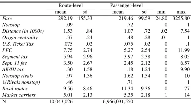
Table 2.1 provides a brief description and source of the main variables used in the analysis. Table 2.2 provides the summary statistics for these variables, including the mean and standard deviation when each route is weighted equally as well as the mean and standard deviation when weighted by passenger volume.
Fare is the average fare of itineraries for ticketing carrier c on route r in market m during periodt. Nonstopequals one if routeris direct service from the origin to destination in its market
m. Distance is defined by the route flown and thus varies across routes within a market. Origin centrality is defined by the origin and carrier on a route. It is the number of nonstop destinations
7Note this is relatively close to the full set of permutations for the included set of airports, approximately 21,000,
and thus close to complete network coverage.
Table 2.1: Variable Description and Sources
Variable Descriptions Source
Fare Mean passenger price on a route DB1B
Nonstop Indicator if nonstop service from origin to destination DB1B
Distance Distance of route flown DB1B
Origin centrality Share of nonstop destinations from origin by a carrier DB1B
U.S. Ticket Tax Ad Valorem tax rate (%) Tax Calculator
PFC Airport specific tax ($) Tax Calculator
Segment tax Segment specific tax ($) Tax Calculator
Sept. 11 fee Per-segment or per-leg specific tax ($) Tax Calculator
AK/HI tax Tax on flights to/from AK/HI ($) Tax Calculator
Nonstop rivals Count of rivals offering direct service DB1B
1(Rivals nonstop) Indicator if any rival offers nonstop service DB1B
Rivals routes Count of rival routes in the market DB1B
Market carriers Carriers in the market DB1B
Note: Outside ofFareandDistance, DB1B variables were constructed from the raw data in the DB1B
Table 2.2: Summary Statistics
Route-level Passenger-level
mean sd mean sd min max
Fare 292.19 155.33 219.46 99.59 24.80 3255.80
Nonstop .09 .72 0 1
Distance (in 1000s) 1.53 .84 1.07 .72 .02 7.54
Origin centrality .37 .24 .48 .28 .01 1
U.S. Ticket Tax .075 .02 .075 .02 0 .1
PFC 7.75 2.74 5.27 2.54 0 11.99
Segment tax 5.94 2.96 3.97 2.38 0 8.05
Sept. 11 fee 3.50 2.67 2.45 2.12 0 6.57
AK/HI tax .30 1.58 .18 1.24 0 9.90
Nonstop rivals .97 1.36 1.62 1.54 0 10
1(Rivals nonstop) .46 .71 0 1
Rival routes 9.56 8.46 11.34 9.36 0 77
Market carriers 5.01 2.13 5.35 2.18 1 14
from the origin by the carrier at timetdivided by the total number of airports. The individual taxes are discussed in greater detail below but briefly, U.S. Ticket Tax is the percentage or ad valorem tax applied to the base fare set by the carrier, whilePFC,Segment tax,Sept. 11 fee, andAK/HI tax
are all specific or dollar-value taxes added to the base fare. All of the tax variables are products of the tax calculator. Nonstop rivalsis the number of rival carriers observed offering nonstop service in market m at time t. The variable 1(Rivals nonstop)is an indicator if any rival offers nonstop service in market m at time t. Rival routes is the number of rival routes in marketm at timet. Finally,Market carriersis the number of carriers providing service in marketmat timet.
2.2.3 Aviation Taxation
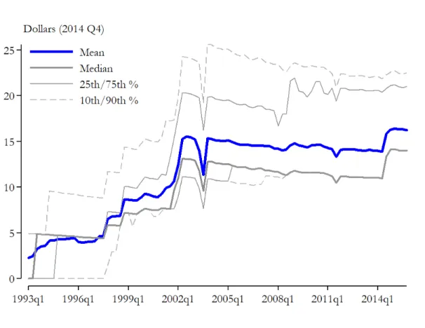
Between 1993 and 2015, taxation in the aviation industry changed dramatically in terms of the amount of taxation on any individual route as well as the type of tax or tax instrument used to raise revenues. Table 2.3 summarizes aviation taxes and how they have changed during the sample period. After a carrier sets a base fare, two types of taxes are directly assessed on domestic flight itineraries: specific or unit taxes, which add a set dollar amount to the base fare, and ad valorem taxes, which add a percentage to the base fare.8 Figure 2.2 displays the mean percentage of a passenger’s fare, inclusive of both specific and ad valorem taxes, remitted to the government. Since the 2nd quarter of 2002, and the introduction of fees related to the 9/11 attacks, taxes or fees compose an average of approximately 15% of a passenger’s fare. As evident from Figure 2.2, this is an approximately 50% increase from the beginning of the sample, when taxes composed less than 10% of a fare.
Four types of specific taxes are potentially applied to domestic itineraries: the U.S. Federal Segment Fee, the Alaska-Hawaii Ticket Tax, the September 11th Security Fee, and Passenger Fa-cility Charges (PFC), many of which were introduced during the sample period. The U.S. Federal Segment Fee was first introduced at $1.00 per non-rural segment in the 4th quarter of 1997 and has steadily increased to $4.00 per non-rural segment in 2015. Flights to and from the continental US and Alaska or Hawaii (or between Alaska and Hawaii) are subject to the Alaska-Hawaii Ticket
8Other taxes, such as corporate income taxes on airline profits or fuel taxes on jet fuel, are not captured by the tax
calculator or directly assessed on itineraries.
Figure 2.2: Tax Share of Fares
Note: This figure graphs the distribution of the share of consumer’s fare attributable to taxes for the years 1993 to 2015. For each quarter it depicts mean, median, 10th, 25th, 75th, and 90th percentiles across passengers. I calculate each statistic at the passenger-level. The plot is conditional on the sample restrictions outlined in Section 2.2.1.
Table 2.3: Summary of Aviation Taxation: 1993 to 2015
Tax Type Change Year Description
U.S. Ticket Ad Lapse 1996 Lack of reauthorization: 0%
Tax Valorem Lapse 1997 Lack of reauthorization: 0%
Statutory 1997-1999 Periodic decline: 10% to 7.5%
Lapse 2011 Lack of reauthorization: 0%
PFC Specific Statutory 2001 Max increased to $4.50
Segment Specific Statutory 1997-2015 Periodic increase: $1.00 to $4.00
September Specific Statutory 2002 Initially $2.50 per segment
11th Fee Lapse 2003 Lack of reauthorization: $0 Statutory 2014 Changed to $5.60 per direction
AK/HI Travel Facilities Tax
Tax, which has ranged from $6.00 in 1993 to $8.90 in 2015. The September 11th Security Fee, depending on the year and quarter, is either $2.50 per-segment with a $5.00 maximum, or $5.60 each direction of an itinerary. Finally, PFCs are airport-specific fees assessed when a passenger enplanes at the designated airport. For an airport to assess the charge, the PFC must be authorized by the FAA. The revenue is treated as local funds and restricted to use on specific long-term capital projects. First authorized in 1992, PFCs initially had a maximum allowable charge of $3.00 per airport. In 2001, the Wendell H. Ford Aviation Investment and Reform Act for the 21st Century increased the maximum charge to $4.50. Figure 2.3 displays the total average specific tax by year and quarter.
Figure 2.3: Specific Taxes
Note: This figure illustrates the distribution of the specific taxes applicable to each fare for the years 1993 to 2015. Specific taxes are measured in dollars. It depicts mean, median, 10th, 25th, 75th, and 90th percentiles. I calculate each statistic at the passenger-level. The plot is conditional on the sample restrictions outlined in Section 2.2.1.
Itineraries in the US are subject to a single ad valorem tax, the U.S. Ticket Tax (also known
as the U.S. Domestic Transportation Tax or U.S. Excise Tax). The ad valorem rate, which in some years varies by an airport’s rural status, is set by the federal government. The tax applies only to portions of the route over the United States. It thus does not apply if the flight goes over international waters or Canada (i.e., involves Hawaii or Alaska). Figure 1.2 shows the effective U.S. Ticket Tax rate from 1993 to 2015. The tax ranges from 0% to 10%. The high volatility in the tax rate where it drops to 0% is due to congressional budget lapses.
2.2.4 Aviation Industry
Passenger aviation has undergone a number of changes during the sample period. Here I pro-vide a broad description of changes along three dimensions; fares and total quantity of passengers, product or route characteristics, and market structure.
Figure 2.4 provides the nominal mean fare for each quarter from 1993 through 2015 as well as the total number of passengers traveling. The average fare has ranged from approximately $142 to $230, with notable persistent declines beginning in 2001 and 2008 corresponding to economic recessions. In terms of passenger volume, outside of the recessionary periods, the total volume of passengers has consistently increased, reaching nearly 96 million in the 4th quarter of 2015. Figure 2.4 also highlights the distinct seasonality, especially in regards to passenger volume, which can make comparisons of consecutive quarters difficult.
Regarding product characteristics, Figure 2.5 displays the percentage of passengers traveling nonstop from their origin to their destination. Even with a visually notable shift during the 2000’s, the percentage of nonstop travel has been fairly steady, between 70 and 75% for most periods. There has been a steady increase in the distance passengers are traveling. As seen in Figure 2.6, passengers have consistently been traveling farther distances, with the average trip increasing from approximately 950 miles in the first quarter of 1993 to over 1,100 miles in 2015. This could be to a greater proportion of travel occurring in markets with geographically dispersed endpoints or consumers selecting longer routes within a given market.
Figure 2.4: Mean Fares and Total Passenger Volume
(a) Fares (b) Passengers
Note: The figures above depict the passenger-weighted mean fare and total number of passengers for the years 1993 to 2015. Panel (a) plots the passenger-weighted mean fare. Fares are at the market level and hence analogous to one-way or half of a round-trip ticket. Panel (b) depicts the total number of passengers. Total passengers is adjusted for the fact the DB1B is a 10% sample of passengers. The plots are conditional on the sample restrictions outlined in Section 2.2.1.
Figure 2.5: Percentage of Nonstop Passengers
Note: This figure plots the mean percentage of nonstop passengers for the years 1993 to 2015. A passenger travels nonstop between an origin and destination when they do not utilize a connecting airport. Within a market, multiple carriers may offer nonstop service. The plot is conditional on the sample restrictions outlined in Section 2.2.1.
Figure 2.6: Mean Route Distance
network. The average number of routes in market increased from between 5 and 5.5 during the mid-1990’s to nearly 7.25 in 2004 before declining to approximately 6.25 during 2015. Similarly, the number of carriers in each market has changed along a similar pattern throughout the period. Before 1998, approximately 3.2 carriers operated on average in each market. Prior to 2008, and the merger of Delta and Northwest, the average number of carriers had risen by 21% to over 3.8 per market. After 2008, carriers per market declined to approximately 2.8 most likely as a result of the mergers of AirTran and Southwest in 2011 and US Airways and American Airlines in 2013.
Figure 2.7: Routes and Carriers per market
(a) Routes per market (b) Carriers per market
Note: The figures above depict the mean number of routes and carriers in each market for the years 1993 to 2015. Panel (a) plots the mean routes per market. A route is the ordered set of airports a passenger utilizes with a particular carrier from their origin to their destination. Panel (b) plots the mean number of carriers per market. As captured by the difference in levels, within a market more routes are observed than carriers on average, indicating the presence of multi-product firms. For each panel, the mean is calculated with each market equally weighted. Within a periodt, the mean is calculated first for each market, and then fortoverall. The plots are conditional on the sample restrictions outlined in Section 2.2.1.
2.3 Empirical Model of Demand and Oligopoly Firms
Directly modeling demand and a firm’s decision-making provides benefits for addressing the complex role of taxes for multi-product firms in a network setting and simulating counterfactual tax policy. I model the U.S. domestic aviation industry using a discrete-choice framework similar to that of Berry (1994) and Berry, Levinsohn, and Pakes (1995). The model is most similar to that of Berry et al. (2006), Berry and Jia (2010), and Ciliberto and Williams (2014), who utilize these
models to analyze the domestic U.S. aviation industry.9 These models view carriers as offering a set of differentiated products, i.e. routes, for markets defined by their origin and destination.
I model demand using a nested logit model. Nested logit models have been used to study a wide range of topics and industries including automobiles (Goldberg 1995; Fershtman et al. 1999), alcohol (Slade 2004), and pharmaceutical drugs (Duso, Herr, and Suppliet 2014). Due to their flexibility and closed-form analytical properties, they are also frequently used to inform policy debates (Werden and Froeb 1994). Unlike the multinomial logit model, which does not allow for consumer responses to be correlated according to a product’s characteristics, the nested logit model allows for correlation across products in a restricted fashion predetermined by the researcher.
On the supply side, the cost for a route is the cost of segments which compose the route, whether the route is nonstop, the characteristics of the endpoints, and an error term meant to capture unexpected random shocks to a route’s cost. The marginal cost of a segment is a function of the total quantity of passengers on the segment. In the airline literature, economies of scale at the segment-level are often described as economies of density.10 Because a segment is an input to many routes, the total quantity of passengers on a route is derived from the costs and demand of many routes.
Carriers compete by choosing prices for their routes. A carrier’s pricing decision balances the potential benefits of economies of scale at the segment level, the marginal cost on a route, and the marginal revenue provided by an additional passenger.
2.3.1 Demand
A nested logit model requires the specification of mutually exclusive sets of products. I nest products (i.e., route-carrier combinations) according to their markets as defined by the origin, final destination, year, and quarter. The utilityuof consumeripurchasing productr(i.e., a route-carrier
9Discrete-choice models have also been used to study a variety of topics in public finance. Bayer et al. (2007)
estimate a household’s willingness-to-pay for school and neighborhood attributes. Fershtman, Gandal, and Markovich (1999) examine counterfactual tax regimes for the Israeli car market.
10Segment-level economies of scale have been well documented in the airline literature. See Brueckner and Spiller
combination) in periodtis
uirt =xrtβ−αpirt+ξrt+νit(σ) + (1−σ)irt, (2.1)
wherexrt is a vector of product characteristics,prt is the price for router in periodt, β captures
the taste for consumers of different characteristics, αcaptures consumers’ disutility from a price increase, andξrt represents a product characteristic unobserved to the econometrician. The term
νit is the “nested logit” random taste, which is constant across airline products and differentiates
air travel from the outside option. The outside option includes not traveling as well as driving, taking a train, or any other non-aviation method of transit.11 The nested logit parameter σ varies between 0 and 1, whereσ = 0reduces the model to the multinomial logit model. Theσparameter captures substitution between flying and the outside option. The termirtis an i.i.d. error intended
to capture idiosyncratic taste for a product. The termνitis distributed such thatνit(σ) + (1−σ)irt
has an extreme value distribution. The mean utility of the outside option is normalized to zero as only differences in utility, not levels, are identified.
Markets are defined to be one-way travel between an origin and destination.12 Thus, a round-trip itinerary will involve products in two markets; the outbound and return legs of the round-trip. As in Berry et al. (2006), Berry and Jia (2010), and Ciliberto and Williams (2014), I define market size as the geometric mean of the origin and destination populations.
Given the assumed structure on the error-term (Cardell 1997), for market m during period t, the proportion of consumers who purchase air travel is
Dmt(1−σ)
1 +D(1mt−σ), (2.2)
11As with most discrete-choice studies, I do not observe the outside option but infer it based on the chosen market
size and observed transactions
12An alternative specification would be to expand either the set of markets or products to differentiate round-trip
from one-way travel. There are two problems with this approach. First, some carriers, such as Southwest, show up in the data as providing only one-way tickets despite providing round-trip travel. Second, computational burden is directly tied to the number of markets and products.
where
Dmt= Rmt X
k=1
e(xktβ−αpkt+ξkt)/(1−σ)
andRmt is the set of routes operated in marketm at timet. Conditional on purchasing a product
from the air travel nest, the probability a consumer purchases productris given by
e(xrtβ−αprt+ξrt)/(1−σ) Dmt
. (2.3)
Thus, the model predictsqrt, productr’s market share at timet, as the probability of choosing air
travel multiplied by the probability of choosing that particular route:
qrt(xmt,pmt,ξmt;β, α, σ) =
e(xrtβ−αprt+ξrt)/(1−σ) Dmt
Dmt(1−σ)
1 +D(1mt−σ). (2.4)
Product characteristics, xrt, include the route’s distance, distance squared, an indicator if the
2.3.2 Marginal Cost
I model the marginal cost of productras the sum overSr, the set of segments which comprise
r:
mcrt= [
X
s∈Sr
c(Qst, wst)] +ωrt,
whereQst captures the total volume of passengers of segments at timetfrom any route andwst
is a vector of exogenous variables such as distance which shift costs. The termwst could include
measures of the direct cost component, such as the additional fuel cost necessary for an added passenger. The termωrt is a product-specific random error term and captures unexpected shocks
to marginal cost such as a shock to fuel cost which disproportionately impacts productr. I do not impose economies of scale in the model or during estimation but specify a segment’s marginal cost,
c(Qst, wst), to be a function of the total quantity of passengers who utilize that segment across all
routes.
Segment marginal cost must be specified flexibly enough that counterfactual analysis is feasi-ble. I utilize a spline function to capture theQst portion ofc(Qst, wst)to recover the relationship
between segment marginal cost and quantity over the support of Q. An increase in segment den-sity,Qst, resulting in lower marginal cost provides evidence of economics of density. The complete
specification of marginal cost is
mcrt=
X
s∈Sr
c(Qst;γs) +
X
s∈Sr
γwwst+γNNr+ωrt, (2.5)
wherec(Qst)captures economics of density at the segment-level and takes the form
c(Qst;γs) =γ0+γ1Qst+γ2(Qst−Q˜25)1[Qst >Q˜25] +γ3(Qst −Q˜50)1[Qst >Q˜50]
+γ4(Qst−Q˜75)1[Qst >Q˜75],
(2.6)
whereQstrefers to the quantity of passengers on segmentsandQ˜25,Q˜50andQ˜75refer to quantity
at the 25, 50, and 75 percentiles of the quantity CDF. The range of potential estimates for a seg-ment’s marginal cost is unrestricted. If the parametersγ1, γ2, γ3, andγ4 = 0, then marginal cost is constant. In equation (2.5),wst includes segment-level characteristics which impact costs such as
distance, distance squared, and centrality of the endpoints. Nris an indicator if routeris nonstop.
Similar to the theoretical model outlined in Brueckner et al. (1992) and Agrawal et al. (2018a), this specification follows Berry et al. (2006) by modeling a route’s marginal cost as the sum of the marginal costs for its segments. This provides an intuitive structure in which cross-product linkages are explicitly captured. For cost complementarities to be a relevant feature of a firm’s profit function, products must be linked by a demand or production relationship.13 Airline products (routes) are linked because the same flight segment (i.e., a flight from airport A to airport B) serves as an input for multiple products or routes (A – B, A – B – C, Z – A – B, etc.). Cost complementarities arise as the cost of operating a segment declines with more passengers due to the use of larger, more fuel-efficient planes and the lower opportunity cost of selling a seat. Thus, cost complementarities arise due to economies of scale at the segment level. These economies of scale incentivize carriers to form hub-and-spoke networks which group passengers with different origins and final destinations onto the same segment, thus driving down the cost for that segment, while also linking products.
2.3.3 Pricing Equilibrium
Conditional on their network, carriers compete by playing a Bertrand-Nash pricing game. In each periodtthey choose a price for each routerto maximize profit:
πct =
X
r∈Rct
prtqrt−
X
s∈Sct
C(Qst)−
X
r∈Rct Trtqrt,
whereRct is the set of routes operated by carrier cat timet, qrt is the quantity of passengers on
route r at time t, Sct is the set of segments operated by carrier c at time t, and Qst is the total
quantity of passengers on segment s. Thus, Qst is the sum of qrt’s where s is a segment on r.
Taxes, which are assessed both at the segment and product level, are captured by Trt. Trt is the
sum of specific taxes applied to routerat timet. The carrier’s choices yieldrfirst-order conditions:
∂πct
∂prt
=qrt+
X
k∈Rcm pk
∂qkt
∂prt
− X
k∈Rcmt X
j∈Sr mcj
∂qkt
∂prt
− X
k∈Rcmt Tkt
∂qkt
∂prt
= 0,
where Rcmt is the set of routes offered by the carrier in market m and Sr is the set of segments
on route r. This first-order condition captures two key aspects the carrier is considering when setting prices; multiple routes within a market and cost complementarities which arise because the same segment appears on multiple routes. First, because routes within a market are substitutes, a change in the price of r is assumed to directly affect demand for other routes in the market, some of which the carrier may operate. As with any multi-product firm, the carrier accounts for the change in profits to its other routes based on the derived substitution patterns specified by the underlying demand system. This could potentially mitigate or amplify price changes relative to a single-product firm. Second, the marginal cost of a route is in part the sum of the marginal cost for each segment on the route. As specified in section 2.3.2, I allow the marginal cost of a segment to be a function of passenger quantity. As a carrier adjusts a route’s fare this will affect the quantity of passengers on that route’s segments and thus the segment’s marginal cost. All segments appear in multiple routes. As their marginal costs change, this affects the underlying pricing decision for other routes. The carrier accounts for these cost spillovers as well.
2.4 Estimation
I jointly estimate demand and supply via GMM. Modeling utility and marginal costs provides two sets of moment conditions, one for each of the structural error terms on a route. LettingZdbe
the set of demand instruments, demand moments take the form
E[∆ξrt(θd)Zd] = 0,
whereθdis the vector of demand parameters to be estimated. Similarly, supply moments take the
form
E[∆ωrt(θs)Zs] = 0,
whereθs is the vector of supply parameters to be estimated andZsthe set of supply instruments.
For demand moments, I model the error term from equation (2.1) asξrt =ξm+ξc+ξt+ ∆ξrt
where fixed effects are captured byξmfor market,ξcfor carrier, andξtfor time fixed effects. Given
my model, the demand error term is
∆ξrt=δrt−αprt−xrtβ−ξm−ξc−ξt, (2.7)
withδrtthe predicted mean utility for the nested logit derived in Berry (1994).
For supply moments, I model the error term from equation (2.5) asωrt=ωc+ωo+ωd+ωt+
∆ωrtwhere supply-side fixed effects areωcfor carrier,ωofor origin,ωdfor destination, andωtfor
time period. The supply error term is
∆ωrt=mcrt−
X
s∈Sr
c(Qst;γ)−
X
s∈Sr
γwst−γ7Nr−ωc−ωo−ωd−ωt. (2.8)
Letgdandgsbe the demand-side and supply-side moments respectively:
gd=E[∆ξZd] =0,
gs=E[∆ωZs] =0,
where∆ξand∆ωare defined by equations 2.7 and 2.8, respectively.