Elastic lattice polymers
M. Baiesi,1,2G. T. Barkema,2,3,4and E. Carlon2 1
Department of Physics, University of Padova, via Marzolo 8, 35131 Padova, Italy 2
Institute for Theoretical Physics, K. U. Leuven, Celestijnenlaan 200D, B-3001 Leuven, Belgium 3
Institute for Theoretical Physics, Utrecht University, Leuvenlaan 4, 3584CE Utrecht, The Netherlands 4Instituut-Lorentz, Universiteit Leiden, Niels Bohrweg 2, 2333 CA Leiden, The Netherlands
共Received 22 February 2010; published 4 June 2010兲
We study a model of “elastic” lattice polymer in which a fixed number of monomersmis hosted by a self-avoiding walk with fluctuating length l. We show that the stored length density m⬅1 −具l典/m scales asymptotically for largemasm=⬁共1 −/m+ . . .兲, whereis the polymer entropic exponent, so thatcan be determined from the analysis ofm. We perform simulations for elastic lattice polymer loops with various sizes and knots, in which we measurem. The resulting estimates support the hypothesis that the exponent is determined only by the number of prime knots and not by their type. However, if knots are present, we observe strong corrections to scaling, which help to understand how an entropic competition between knots is affected by the finite length of the chain.
DOI:10.1103/PhysRevE.81.061801 PACS number共s兲: 36.20.Ey, 02.10.Kn, 87.15.A⫺
I. INTRODUCTION
According to renormalization group theory, the scaling properties of critical systems are insensitive to microscopic details and are governed by a small set of universal expo-nents 关1兴. Also polymers can be considered as critical sys-tems in the limit where their lengthl共the number of chained monomers兲diverges 关2–4兴. For instance, the radius of gyra-tion of an isolated polymer in a swollen phase scales asRg
⬃l, where⬇0.587597共7兲 关5兴ind= 3 dimensions is a uni-versal critical exponent. One of the simplest models in the universality class of swollen polymers is that of self-avoiding walks共SAWs兲on a lattice. Hence, these have been used extensively to extract information on critical exponents and scaling functions关2,4–23兴. The total number of SAWs, i.e., their partition function, has the following large-l expan-sion
Zl⬃ll共1 +Al−⌬+ . . .兲. 共1兲
Here, nonuniversal共model-dependent兲quantities are the con-nectivity constant and the amplitude of the corrections to scaling A. Theentropicexponent depends only on bound-ary conditions: ind= 3 we have⬅␥− 1 = 0.1573共2兲 关24兴for an open chain whereas ⬅␣− 2 = −d= −1.762791共21兲 关5兴 for self-avoiding polygons共SAPs兲, that is, linear chains with the two ends on adjacent lattice sites. Renormalization group analysis suggests that the exponent ⌬, characterizing the leading corrections to the scaling behavior, is also universal 关1,3兴
Models with full self-avoidance, such as SAPs, have been used to study the statistical properties of knotted chains 关13,14,19,25–35兴. Knots in polymers have attracted a lot of attention during the past years, also because of their occur-rence in biopolymers as DNAs, RNAs, and proteins关36–41兴. As usual, SAWs represent a minimal effective model to grasp the essential, coarse-grained features of polymer chains. Simulations of knotted SAPs in ensembles with fixed topology are performed with a grand-canonical algorithm 共BFACF 关6兴, from the name of the authors兲tuned to span a
range of chain lengths 共algorithms with fixedN are not er-godic in this case兲. For this algorithm, the tuning of step fugacities to u⬇1/ is necessary to achieve samplings of long chains. It would be desirable to have a simpler and more stable method to sample the same chain lengths.
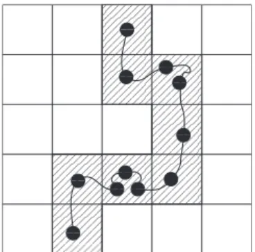
In this paper, we study a class of polymers referred to as the elastic lattice polymers 共ELPs兲, which are SAWs accu-mulating some stored length along their contour. This leads in fact to a partial lifting of the self-avoidance condition between consecutive monomers of an ELP, as sketched in
Fig.1. We will consider equilibrium properties of polymers
with a fixed number of monomers m, and in which as a consequence the length lⱕmof the self-avoiding backbone described by the monomers fluctuates. This explains the name “elastic,” and implies a resemblance with the class of grand-canonical SAW models.
There are several reasons for studying this model. On the theoretical side, it can be considered as an enhanced SAW: besides sharing critical exponents with SAWs, its fluctuating length enables new avenues to estimate critical exponents. ELPs have been used in studies of polymer dynamics as phase separation in polymer melts 关22兴, or in translocation through nanopores关21兴, but their equilibrium properties have so far received little attention. The key quantity we focus on
0 0 0 0 0 0 0 0 0 0 0 0 0 0 0 0 0 0 0 0 0 0 0 0 0 0 0 0 0 0 0 0 0 0 0 0 0 0 0 0 0 0 0 0 0 0 0 0 0 0 0 0 0 0 0 0 0 0 0 0 0 0 0 0 0 0 0 0 0 0 0 0 0 0 0 0 0 0 0 0 0 0 0 0 0 0 0 0 0 0 0 0 0 0 0 0 0 0 0 0 0 0 0 0 0 0 0 0 0 0 0 0 0 0 0 0 0 0 0 0 0 0 0 0 0 0 0 0 0 0 0 0 0 0 0 0 0 0 0 0 0 0 0 0 0 0 0 0 0 0 0 0 0 0 0 0 0 0 0 0 0 0 0 0 0 0 0 0 0 0 0 0 0 0 0 0 0 0 0 0 0 0 0 0 0 0 0 0 0 0 0 0 0 0 0 0 0 0 0 0 0 0 0 0 0 0 0 0 0 0 0 0 0 0 0 0 0 0 0 0 0 0 0 0 0 0 0 0
1 1 1 1 1 1 1 1 1 1 1 1 1 1 1 1 1 1 1 1 1 1 1 1 1 1 1 1 1 1 1 1 1 1 1 1 1 1 1 1 1 1 1 1 1 1 1 1 1 1 1 1 1 1 1 1 1 1 1 1 1 1 1 1 1 1 1 1 1 1 1 1 1 1 1 1 1 1 1 1 1 1 1 1 1 1 1 1 1 1 1 1 1 1 1 1 1 1 1 1 1 1 1 1 1 1 1 1 1 1 1 1 1 1 1 1 1 1 1 1 1 1 1 1 1 1 1 1 1 1 1 1 1 1 1 1 1 1 1 1 1 1 1 1 1 1 1 1 1 1 1 1 1 1 1 1 1 1 1 1 1 1 1 1 1 1 1 1 1 1 1 1 1 1 1 1 1 1 1 1 1 1 1 1 1 1 1 1 1 1 1 1 1 1 1 1 1 1 1 1 1 1 1 1 1 1 1 1 1 1 1 1 1 1 1 1 1 1 1 1 1 1 1 1 1 1 1 1
0
0
1
1
0
0
1
1 0011
0
0
1
1
0
0
1
1
0
0
1
1
0
0
1
1
0 0 0 0 0 0 1 1 1 1 1 1
0
0
1
1
0
0
1
1
0
0
1
1
is the equilibrium averaged stored length density defined as
m⬅ m−具l典
m , 共2兲
where具l典depends onm. As will be shown,mhas a simple asymptotic behavior for largemfrom which one can extract universal exponents: the leading correction to the asymptotic value formscales as/m, whereis the entropic exponent defined by Eq. 共1兲. We illustrate the result of this approach for the case of ELPs with fixed knots. If knots are present, the stored length approaches its asymptotic value with strong, knot-dependent corrections to scaling. The expecta-tion of a homogeneous stored length within an equilibrated chain, combined with the knowledge on how its density var-ies with the chain length, leads us to a new view on the issue of entropic competition of knotted regions 关25兴. On the nu-merical side, we find that ELPs, compared to grand-canonical algorithms, have the nice feature of stabilizing the sampling quite narrowly around an easily tunable length具l典. This paper is organized as follows. In Section II, we de-rive the expansion formas a function ofm. In Section III, we illustrate how to estimate entropic exponents via fits of
m, with a reweighting of exact enumeration data for poly-mers on square and cubic lattices. In SectionIV, we present Monte Carlo simulations of ELPs containing a fixed knot and determine the averaged stored length in equilibrium as a function of m. The entropic exponent is determined for different simple and double knots. Finally, in SectionV, we discuss, on the basis of the obtained scaling behavior form, different possible scenarios for knot competitions.
II. SCALING PROPERTIES OF THE STORED LENGTH
Consider a polymer composed bym monomers with lat-tice coordinates defined by rជi, i= 1 , 2 , . . .m. Multiple occu-pancy of neighboring monomers on the same lattice site means that we allow configurations for which rជk=rជk+1= . . . =rជk+p=sជ. However ifrជk−1⫽sជ andrជk+p+1⫽sជ, then no mono-mers other than those of the interval关k,k+p兴are allowed to visit the site sជ. The lattice polymer so defined describes a self-avoiding backbone of length 0ⱕlⱕm. The two extremal cases are all monomers occupying the same lattice point 共l= 0兲 and a fully stretched configuration without multiple occupancy 共l=m兲. The equilibrium partition function for an ELP withmmonomers is given by
Z ˜
m=
兺
l=0
m
冉
m l冊
ulZ
l, 共3兲
where the sum is over the lengthlof the self-avoiding back-bone andZlis the canonical partition function, which counts
the number of allowed configurations for the self-avoiding backbone, and whose asymptotic is given in Eq. 共1兲. The factor 共ml兲 in Eq.共3兲counts the number of ways the stored length can be distributed over the backbone. For convenience an extra fugacityu per site has been added.
Substituting Eq. 共1兲 in Eq. 共3兲 and defining =u, the average backbone length具l典can be computed from
具l典=
log˜Zm. 共4兲
It is instructive to consider first the case of a partition function of the typeZl=lin Eq.共3兲, i.e., neglecting
power-law and correction to scaling terms in Eq. 共1兲. In this case Eq. 共3兲becomes
Z ˜
m ⬁=
兺
l=0
m
冉
m l冊
l
=共1 +兲m. 共5兲
Equation 共5兲 has the following interpretation: the partition function for a walk of m steps factorizes as each monomer can either sit on the backbone 共accumulating stored length with weight 1兲or occupy a free site共with average weight兲. From Eq. 共4兲 we get the following value of the averaged backbone length
l⬁= m
1 +. 共6兲
We now go back to the full partition function in Eq.共3兲. For largemand fixedthe binomial factor is sharply peaked around l=l⬁. We approximate the binomial by a Gaussian distribution as follows:
冉
m l冊
l⬇ 共
1 +兲m
冑
1 22e−共l−l⬁兲2/22
, 共7兲
where
2= m
共1 +兲2. 共8兲 The Gaussian approximation differs from the binomial by terms which are exponentially small for large m, which are of higher order in the large-mexpansion we are interested in, so they can be safely neglected. We replace now the discrete sum in Eq.共3兲by an integral over all lengths, extending the domain of integration in the whole real axis:
Z ˜
m=
共1 +兲m
冑
22冕
−⬁
+⬁
dle−共l−l⬁兲2/22l共1 +Al−⌬兲, 共9兲
where we have replaced the asymptotic form of Zl as given
in Eq.共1兲. The replacement of the sum by an integral brings corrections in Eq.共9兲, which are of higher order in 1/mand for our purposes can be neglected.
We solve the integral in Eq. 共9兲 by using a saddle point approximation. A simple rescalingl=xl⬁gives
Z ˜
m=共1 +兲m
冑
m 2
冕
−⬁+⬁
dxem⌫共x兲 共10兲
with
⌫共x兲=−共x− 1兲 2
2 +
log共xl⬁兲+ log共1 +A共xl⬁兲−⌬兲
m .
Z ˜
m⬇ 共1 +兲m
冑
m 2e
m⌫共¯x兲
冑
2m兩⌫
⬙
共¯x兲兩=共1 +兲me
m⌫共¯x兲
冑
兩⌫⬙
共¯x兲兩. 共12兲Equation 共11兲 implies that the maximum of ⌫共x兲 in the large-mlimit is¯x= 1 +O共1/m兲, giving
兩⌫
⬙
共¯x兲兩= 1 +O冉
1m
冊
, 共13兲which produces higher-order terms, which we neglect in the large-mexpansion. In addition:
m⌫共¯x兲=logl⬁+ log共1 +Al⬁−⌬兲+ . . . 共14兲 Equations共12兲–共14兲again show that the leading contribution to the partition functionZ˜mis共1 +兲m, but also that the
sub-leading contribution ⬃l⬁⬃m has the same entropic expo-nent of SAWs. From Eq.共4兲we get
具l典=l⬁
冋
1 + m−A m
冉
1 + m
冊
⌬
册
共15兲and the stored length density Eq. 共2兲becomes
m=⬁
冋
1 − m+冉
1 +
冊
⌬ A
m1+⌬
册
, 共16兲 where we defined⬁=
1
1 +. 共17兲
The expansion Eq. 共16兲is valid provided⌬⬍1. The ne-glected terms coming from the replacement of the sum with an integral, and from the Gaussian integration in Eq. 共10兲, are of the order 1/m2 共except if ⌬⬎1, the O共1/m2兲 terms would dominate over the 1/m1+⌬.兲The value of the exponent
can then be obtained from a plot ofmvs 1/m, as the slope in the limit 1/m→0. Using the high-precision literature val-ues for the connectivity constants , one obtains a very ac-curate estimate of⬁.
With the definition of ⬁ in Eq.共17兲 we can rewrite the variance Eq.共8兲as
2=m
⬁共1 −⬁兲. 共18兲
This form reveals clearly that the largest for a givenmis achieved with⬁= 1/2, i.e., with a fugacityu=−1. We can think of this regime as the maximally elastic one. In all cases, note that the relative polydispersity/mof the chains goes to zero⬃m−1/2form→⬁, hence the chain lengthslare narrowly distributed around their average具l典. This allows us to use saddle-point approximations共see Sec.V兲and leads to metric properties in the universality class of SAWs 共e.g., radius of gyration scaling as⬃m⬃具l典兲. Hence, ELPs share both exponents and with SAWs.
III. STORED LENGTH FROM EXACT ENUMERATIONS DATA
As a first illustration of the scaling behavior of the stored length m as a function of the number of monomers m, we consider exact enumeration data for SAWs and SAPs on square and cubic lattices, which are taken from the published literature关17兴. Enumeration techniques provide exact values for the total number of SAWsZlas a function of their length
l. We use these values forZlto computeZ˜mfrom Eq.共3兲. The
stored length mis obtained from the average 具l典, using Eq. 共2兲. We have the freedom to choose the value of the fugacity u in Eq.共3兲.
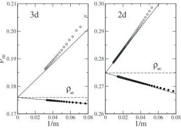
Figure2shows a plot ofmas a function of 1/mfor three and two dimensions, obtained by settingu= 1 in Eq.共3兲. The data converge to the expected asymptotic value, which is
⬁⯝0.175931 共cubic兲 and ⬁⯝0.2748643 共square兲. These are obtained from Eq.共17兲with=u=and the following values for the connectivity constants: = 4.684044共11兲 关20兴 共cubic兲and= 2.63815852927共1兲 共square兲 关16兴.
The solid lines in Fig.2are the linear terms in the expan-sion of Eq.共16兲where the value of is that for open walks 共= 11/32 in d= 2 and ⯝0.157 in d= 3兲 and polygons 共= −3/2 in d= 2 and ⯝−1.76 in d= 3兲. The results show that the linear scaling in 1/msets in already for short poly-mers共m⬇20兲. In addition we observe that the corrections to the leading scaling behavior are stronger for closed walks 共empty circles兲 compared to the open walks case 共filled circles兲.
We performed finite-size extrapolations to obtain esti-mates of from m. The two-dimensional data have been extrapolated by means of the Burlisch-Stoer共BST兲algorithm 关42兴, using the finite-m approximants
m⬅ m−m−1
m−1/m−m/共m− 1兲
, 共19兲
which are the ratios between slope and intercept of the line joining the points 共1/共m− 1兲,m−1兲 and共1/m,m兲, i.e., they
0 0.02 0.04 0.06 0.08
1/m
0.17 0.18 0.19 0.20 0.21
ρ m
3d
ρ
80 0.02 0.04 0.06 0.08
1/m
0.26 0.27 0.28 0.29 0.30
2d
ρ
8are finite-size estimates of the ratio between⬁and⬁. The BST algorithm starts with a sequence of N elements, and generates iteratively sequences of N− 1, N− 2. . . elements which are expected to converge faster at each iteration step. It involves a free parameter共⍀兲, which roughly measures the effective leading correction exponent. In our extrapolations, an optimal value of⍀was selected requiring a minimal stan-dard deviation of the last five sequences generated by the iterative algorithm. The extrapolations were repeated for dif-ferent values of the fugacity parameter u and the error was estimated from the variation on these values. For three-dimensional data, the BST algorithm turned out not to be very accurate, particularly for loops. The reason is thatmfor small mhas some subleading oscillatoric behavior which is not sufficiently damped during the BST iterations. The result is that the accuracy of the extrapolation is poor. For these data we use instead a nonlinear fit, fixing⬁and keeping, A, and⌬as fitting parameters.
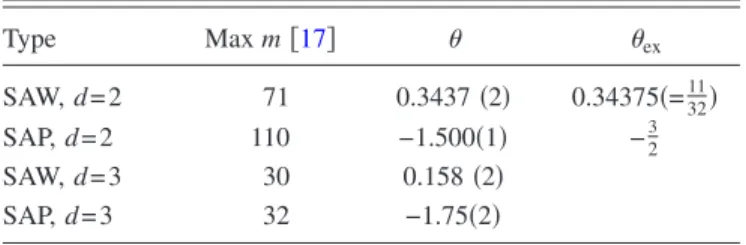
The extrapolated values for are reported in Table I; these are accurate and in good agreement with exact data in two dimensions and also with the best numerical estimates in three dimensions 共= 0.1573共2兲 关24兴 for walks, = −1.76279共2兲 for polygons—assuming hyperscaling ␣− 2 = −d with = 0.587597共7兲 关5兴兲, which shows that reliable values of the entropic exponents can be extracted from the scaling of the stored length.
IV. ENTROPIC EXPONENTS OF KNOTTED POLYMERS
We now turn to the study of equilibrium properties of ELP rings with some fixed topology. Here, we will show how the knowledge of the stored lengthmcan be exploited to investigate equilibrium properties of knotted polymers.
We have performed Monte Carlo simulations of ELPs on the face-centered-cubic 共fcc兲 lattice, with an algorithm that was recently used to study translocation dynamics关21兴 and phase separation in polymer melts关22兴. The allowed Monte Carlo update moves include reptation, i.e., the diffusion of stored length along its backbone and Rouse-like moves, which locally change the backbone configuration.共For more details see Ref.关22兴.兲.
The setup of the simulation is as follows. We start from a backbone with a minimal number of steps on the fcc lattice, as those shown in Fig.3. A total number of monomersmare distributed randomly over this backbone. These configura-tions are then relaxed to equilibrium. Typically m is much
larger than the initial length共we simulated polymers withm up to 2000兲so that relaxation to equilibrium corresponds to an expansion of the backbone. The Monte Carlo moves pre-serve the knot topology imposed initially. Once equilibrium is reached we start the sampling of the stored length density
m.
An additional weight共equal to 4兲is introduced for moves that accumulate monomers on the same lattice point, which corresponds to a fugacity factoru= 1/4 in Eq.共3兲. This leads to the following asymptotic value for the stored length den-sity:
⬁= 1
1 +/4= 0.28498共1兲, 共20兲 where the numerical value is obtained by considering the most accurate available estimate = 10.0362共6兲 关9兴 for the connectivity constant of SAWs on fcc lattice关47兴.
Figure4shows the scaling behavior ofmas a function of 1/m for an unknotted polymer ring, for single and double knots. All data converge asymptotically to the value ⬁ ob-tained from Eq. 共20兲. This value is shown as a dashed hori-zontal line in Fig. 4. We note that the approach to⬁of the numerical data for unknotted rings is quite different for those of rings with knots 共a detail of the asymptotic region is shown in the inset of Fig. 4兲: the data for the unknotted topology approach the asymptotic value with a clear 1/m scaling behavior. For topologies with knots instead there is a pronounced curvature in the mvs 1/mplot, deriving from strong corrections to scaling. These corrections are stronger for an increasing knot complexity and for an increasing num-ber of knots. The shortest lengthlminof a knot on a lattice is a good indicator of its complexity, and in this model for m =l=lmin by definition the chain can only be fully stretched, i.e., m
min= 0. Our data show that the crossover from this
initial topological stretching to the asymptotic regime⬃m−1 grows quickly with the value of mmin. In this view, the fact that for unknotted chains on the fcc lattice one hasmmin= 3, much smaller than that of the simplest knot共the trefoil with mmin= 15兲explains why corrections to scaling are negligible for unknotted chains.
We estimated the entropic exponent using the scaling behavior predicted by Eq.共16兲. In the unknotted case due to
TABLE I. Summary of the exponents obtained from the ex-trapolation of the approximantsmdefined in Eq.共19兲. The data are for SAWs and SAPs 关17兴. The last column gives the exact two dimensional data关4兴.
Type Maxm关17兴 ex
SAW,d= 2 71 0.3437共2兲 0.34375共=1132兲
SAP,d= 2 110 −1.500共1兲 −23
SAW,d= 3 30 0.158共2兲
SAP,d= 3 32 −1.75共2兲
(b) (a)
FIG. 3. 共Color online兲Examples of knots on the fcc lattice:共a兲 a 31knot共trefoil兲withl= 15 steps and共b兲a composite 31# 41knot withl= 31 steps共the notationk1#k2indicates a closed polymer ring
the manifest absence of curvature of the data, we restricted ourselves to a linear fit settingA= 0 and⬁= 0.28498 in Eq. 共16兲and usingas the only free parameter. The fit, restricted tomⱖ200, yields= −1.76共3兲, confirming that the entropic exponent for rings with fixed unknotted topology is identical to that for SAPs with no topological constraints.
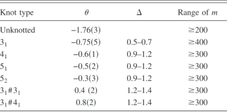
A closer look at the data reveals that the stored length density for knots 31, 41and 51is nonmonotonic. As the data asymptotically approach ⬁ from above, Eq. 共16兲 implies a negative value of the exponent. We performed a nonlinear three-parameters fit to the databased on Eq.共16兲:,⌬andA are fitting parameters while we fix⬁= 0.28498, as predicted by Eq. 共20兲. The results of the nonlinear fits are given in Table II. The estimated exponent changes sign from single knot共⬍0兲to double knots 共⬎0兲. A range of correction-to-scaling exponents ⌬ providing optimal fits were selected and these are given in the third column of Table II. Error
estimates for reflect the variability in from the different values of ⌬ used in the analysis. For the knots studied, the most accurate estimate for is that of the 31 knot, yielding
= −0.75共5兲. The error increases with the knot complexity. For single knots we also note a change in the range of correction-to-scaling exponents from⌬⬇0.6 for the 31knot to⌬⬇1.1 in the other knots.
It has been suggested关13,14,35兴that for a knotkwithk prime components, the entropic exponent is given byk= +k, where is the exponent for a polymer ring without fixed topology. If this is the case we expect for a single knot an exponent = −3+ 1 = −0.76 while for double knots
= −3+ 2 = 0.24 共these conjectured values are shown as dashed lines in the inset of Fig. 4兲. The idea behind this suggested scaling is that localized knots are like sliding en-tities, which can occupy any of the l sites of a chain, thus contributing entropically with a factorlin the partition func-tion. Our numerical results fully support this conjecture for the single 31 knot and also for the double 31# 31 knot. Re-sults for the other knots seem to overestimatewith respect to the conjectured values. It is likely that the deviations from the conjectured values are due to strong finite-size effects. An indication of this is the value of the correction-to-scaling exponent obtained from the fits, which, with the exception of the 31 knot, is estimated as ⌬⬇1. Renormalization group arguments 关1兴 for magnetic O共N兲 models, which map into polymer models in the limit N→0 关2兴, predict instead ⌬ ⬇0.55, and Clisby 关5兴finds⌬⬇0.528共12兲in simulations of very long SAWs共this is in agreement with the range of val-ues obtained in the extrapolations of the numerical data for the 31 knot, see Table II兲. We also remark that a value ⌬
⬎1 is at odds with the expansion of the stored length of Eq. 共16兲 in which it was implicitly assumed ⌬⬍1, the 1/m1+⌬ term would be otherwise dominated byO共1/m2兲corrections, which were neglected in the computation of m leading to Eq. 共16兲.
In the sequel we fix the entropic exponents to the conjec-tured values¯⬅−3+k and subtract frommthe constant and leading correction in 1/mas
fm⬅m−⬁
冉
1 − ¯
m
冊
. 共21兲For this quantity we expect the following scaling behavior
fm⯝
A ¯
m1+⌬+ B ¯
m2, 共22兲
where a next-order 1/m2term has been added.
Figure5plotsfmm1+⌬, where we set⌬= 0.5, as a function
ofm. The fact that this quantity approaches a constant value for largemsupports an estimate of the correction-to-scaling exponent ⌬⬇0.5, as expected for swollen polymers关4兴. In addition the constantA¯ is negative and its magnitude quickly increases with knot complexity. This is also visible in Fig.4 as the effect of increasingAis that of producing an increased curvature in a plot ofmvs 1/m. It is perhaps not surprising that finite-size effects increase with the knot complexity, as more complex knots are expected to occupy a larger portion
0 0.01 0.02 0.03 0.04 0.05
1 / m
0.22 0.24 0.26 0.28 0.3
ρ m
0 0.001 0.002 0.284
0.285 0.286
31 4
1
51 52 3
1#31
31#41
unknotted ρoo
θ=-1.76 θ= -0.76
θ= 0.24
FIG. 4. 共Color online兲 Plot of the average equilibrium stored length density m as a function of the inverse monomer number 1/mfor closed polymers with some fixed topology. The simulations were extended to polymers of lengths up tom= 2000. From top to bottom the data refers to: unknotted ring, 31, 41, 51, and 52knots.
The two bottom data set correspond to configuration with two knots: 31# 31and 31# 41, respectively. The horizontal dashed line is ⬁= 0.28498, as expected from Eq. 共20兲. Inset: zoom of the
asymptotic region. Straight lines represent⬁共1 −/m兲: the dotted line corresponds to the conjectured value= −3, the dashed line to
= −3+ 1, and the dot-dashed line to= −3+ 2.
TABLE II. Summary of the estimated entropic exponents ob-tained from the scaling behavior of the stored length with a three parameters fit关,⌬andAin Eq.共16兲兴. The asymptotic value⬁is kept fixed. The last column shows the range of polymer sizes used in the fit.
Knot type ⌬ Range ofm
Unknotted −1.76共3兲 ⱖ200
31 −0.75共5兲 0.5–0.7 ⱖ400
41 −0.6共1兲 0.9–1.2 ⱖ300
51 −0.5共2兲 0.9–1.2 ⱖ300
52 −0.3共3兲 0.9–1.2 ⱖ300
31# 31 0.4共2兲 1.2–1.4 ⱖ300
of the polymer. In TableIII, we list our estimates ofA¯ andB¯, obtained by means of linear fits to data in the form fmm1.5vs
m−0.5. The values ofB¯ are almost two orders of magnitude larger than those ofA¯, explaining the fitted共effective兲 lead-ing exponent⌬⬇1.
V. KNOTS COMPETITION
In this section, we discuss entropic competition between knotted polymers in the context of ELPs. The idea of en-tropic competition between polymers with various con-straints was introduced in Ref.关25兴. as a direct way to esti-mate polymer entropic exponents from canonical simulations. This idea is sketched in Fig.6and can be imple-mented in various ways. One can consider, for instance, a polymer loop divided in two sides by a wall关Fig.6共a兲兴; the two sides exchange monomers via sufficiently small holes such that the knots cannot pass through. The exchange can also occur through a fictitious “wormhole”关25兴, as shown in Fig.6共b兲. The polymers at the two sides of the wall or those exchanging monomers through the wormhole do not interact with each other. When exchanging monomers the length of each loop fluctuates, while the total length is fixed to a con-stant L. The method 关25兴 is based on the analysis of the equilibrium distribution of lengths of the two sides. For or-dinary polymers one expects that the lengthlof one polymer ring is distributed according to
p共l兲 ⬃Zl共
1兲Z
L−l
共2兲 ⬃L
l1共L−l兲2, 共23兲
where the two Z’s are the loop partition functions given in Eq. 共1兲. The main point is that the dependence onin Eq. 共23兲is irrelevant asLis fixed, whereas from the analysis of the shape of the probability p共l兲 as a function oflit is pos-sible to fit the values of the entropic exponents1 and2of the two loops关25兴.
A. Entropic competition without a wall
We first consider the case depicted in Fig. 6共b兲, and we discuss a few representative examples. If the two loops both have negative entropic exponents 共1,2⬍0兲, then one ex-pects a p共l兲 as depicted in Fig. 7共a兲共thick line and shaded area兲, whereas the case 1,2⬎0 is depicted in Fig. 7共b兲 关same notation; in these figures, for convenience we show the distributionp共l/L兲, which is just a rescaling ofp共l兲兴. The thin lines in Figs. 7共a兲 and 7共b兲 show sketches of finite-L
1.5 2 2.5 3 3.5
log10m
-30 -20 -10 0
fm
m
1.
5
unknot 31 41 51 52 31#31 31#41
FIG. 5. 共Color online兲Plot offmm1+⌬vs log10m, with⌬= 1/2.
The data tend to a constant for largem, which, as discussed in the text, is consistent with a correction-to-scaling exponent of⌬⬇0.5.
TABLE III. Fits ofA¯ andB¯, assuming⌬= 1/2 in Eq.共22兲.
Knot type A¯ B¯
31 −0.78 −33
41 −1.9 −63
51 −3.5 −73
52 −4.1 −80
31# 31 −1.4 −130
31# 41 −3.3 −173
(b) (a)
FIG. 6. 共Color online兲 共a兲 Sketch of an entropic competition: a portion of the ring polymer, with two knots, is constrained to stay on the left half-space共holes are small enough to forbid more than one monomer at a time to pass兲, the remaining part has one knot and is on the other side of the wall. The total lengthNof the chain is constant but the lengths mand N−mof the two subchains can fluctuate. 共b兲 The virtual version 共without the wall兲 of the same competition: the two polymers swim in separate dilute solutions and are coupled via a “wormhole” trough which they can exchange a monomer共hence not a knot兲at a time.
0 0.2 0.4 0.6 0.8 1
l/ L
-1 0 1
log
10
P(
l
/L
)
short L
L−−>oo
short L
0 0.2 0.4 0.6 0.8 1
l/ L L−−>oo
(a) (b)
FIG. 7. 共Color online兲Examples of probability distributions of loop lengths for two polymer loops exchanging monomers as in Fig. 6共b兲, in the case of negative共a兲and positive 共b兲entropic ex-ponentfor both loops. In共a兲the competition is between two 31 knots, the thick line共boundary of the shaded area兲is the distribution for the limit of longLwhile the other ones are for two shortL’s. In 共b兲the competition is between a 31# 31knot and a 31# 41knot, with
distributions of p共l兲for increasingL: particularly interesting is the scenario depicted in Fig. 7共a兲, which shows a drastic change of the shape of the distribution from a finiteLto the limitL→⬁. We will discuss here how some of these features can be understood from the analysis of the stored length densities m共1兲andm共2兲of the competing loops.
Let us considerp共m兲, the probability of findingm mono-mers in one of the two entropically competing ELP loops. This quantity scales as
p共m兲 ⬃˜Zm共
1兲Z˜
N−m
共2兲 , 共24兲
where the twoZ˜s are the partition functions of the two com-peting ELPs at fixed monomer numbers m and with fluctu-ating lengths. To find the most probable value of the mono-mer number mⴱ observed in the entropic competition setup, we maximize the entropy
Sm=kBlog˜Zm共
1兲+k
BlogZ˜N共−m
2兲 共25兲
共kB is the Boltzmann constant兲. The partition functions of
ELPs in Eq. 共3兲 are expressed as a sum over all lengths 0
ⱕmⱕl. The sum is however dominated by a characteristic value oflⴱ共m兲 obtained from the condition
冏
˜Zm,l l冏l
=lⴱ共m兲= 0, 共26兲
where we defined Z ˜
m,l⬅
冉
m l
冊
ul
Zl. 共27兲
Now assuming that ˜Zm is dominated by a single value of
lⴱ共m兲we can compute the total derivative inmof log˜Zmas
dlogZ˜m
dm ⬇
dlog˜Zm,lⴱ共m兲
dm =
logZ˜m,lⴱ共m兲 m
= d dmlog
m!
关m−lⴱ共m兲兴!= − logm. 共28兲 In this derivation we used Eq.共26兲, so in the total derivative with respect to mwe can ignore the m-dependence coming from lⴱ共m兲. Combining Eqs.共25兲 and共28兲 we find that the extremum of the entropySmof the competing rings is given
by the value ofmⴱ for which
m共1ⴱ兲=N−mⴱ
共2兲
. 共29兲
To findmⴱone can plotm共1兲 andN共2−兲mvsmandN−min the
same graph: each intersection point between the two curves is an extremum of Sm. To decide whether this is a local
maximum or minimum one analyzes the second derivative
冏
d2Smdm2
冏
mⴱ⯝− 1
m共1ⴱ兲
冋
dm共1兲 dm −
dN共2−兲m
d共N−m兲
册
mⴱ. 共30兲
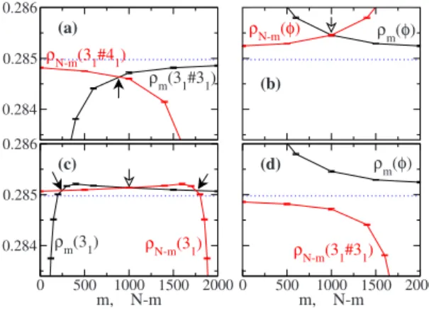
In Fig.8, we show some plots of the stored-length densi-ties for the two competing loops containing knots. The two loops have a total number of monomers equal to N= 2000 and the data are those shown in Fig. 4, but now plotted as
function ofmandN−m. As seen in the previous section, the stored length density can be nonmonotonic in m for some knotted configurations, which can produce various scenarios where up to three intersection points are possible.
Figure 8共a兲shows the example of two competing double knots. In this case there is a single intersection point and the analysis of the first derivatives ofshows that this point is a local maximum for the entropy 关Eq. 共30兲兴. The probability distribution of monomers 共or lengths in the canonical setup兲 will have a single maximum at some intermediate mⴱ, as shown in the example of Fig. 7共b兲. In the case of two un-knotted loops关Fig.8共b兲兴the intersection point mⴱis a mini-mum for the entropy, hence the probability distribution form will be maximal at the edges and minimal at mⴱ, as for the thick line in Fig. 7共a兲. The most interesting case is that of competition between loops with nonmonotonic’s. This case is illustrated in Fig. 8共c兲. The three intersection points are a central local minimum of the entropy enclosed by two local maxima. The probability distribution of lengths is like that depicted as a dashed line in Fig.7共a兲. It is easy to see that if the total number of monomers decreases共this corresponds to shift one of the two ’s along the horizontal axis兲there will be only one intersection point. This generates a probability distribution with a single maximum formⴱ关thin dense line in Fig. 7共a兲兴. Interestingly, the length distributions obtained from Monte Carlo simulations 关25兴of competing off-lattice flexible rings with simple knots give, for sizes up to 200 monomers, concave distributions, contrary to the expecta-tions of negative’s from the conjecture of Ref.关13兴, which would instead correspond to a convex共i.e., with a minimum in the middle兲 shape. The nonmonotonicity in m of the stored-length density mexplains this drastic change in be-havior in finite-size data.
To complete the discussion, we consider next an example where no intersection point is present关Fig.8共d兲兴. In this case one has to resort to the full form ofSm: from the scaling of
partition functions of SAPs, the probability of a state withm monomers on the side with no knots is expected to scale as
0.284 0.285 0.286
ρm(31#31)
ρN-m(31#41)
ρm(31) ρN-m(3
1)
ρm(φ)
ρN-m(31#31)
(a)
(b)
0 500 1000 1500 2000
m, N-m
0.284 0.285 0.286
(c)
0 500 1000 1500 2000
m, N-m
(d)
ρm(φ)
ρN-m(φ)
FIG. 8. 共Color online兲Plot of stored-length densities vsmand
N−min the entropic competition setup, for four different knotted chains:共a兲31# 31vs 31# 41,共b兲unknot vs unknot,共c兲31vs 31, and
m−3⬃m−1.76with a cutoff atmⱗN. It implies that the aver-age length of the unknotted subchain 具m典N⬃N␣⬃N0.24 is
weakly scaling withN, and at least in this case the competi-tion is clearly in favor of the side with knots. This reminds us that the full statistics given bySmwould often be necessary
to compute average quantities, and that the maxima are only indicative elements. Nevertheless, we have seen that the den-sity of stored length is a useful quantity for understanding the basic properties of the entropy of competing knotted chains. In particular, knowing it and its short-N features helps to interpret the numerical results and to distinguish preasymptotic scalings from asymptotic ones.
B. Entropic competition with a wall
Let us finally go back and reconsider briefly the entropic competition of knots divided by a wall, as in Fig.6共a兲. The main difference is that the basic exponent of the unknotted chain should bes= −d+2
⬘
. The additional index2⬘
is nected to the constraint of having a monomer of a loop con-fined close to a hard surface. The formula is an application of Duplantier’s general theory of polymer networks关43,44兴. We use this theory also to extract2⬘
from the data in Ref.关45兴, obtaining2⬘
⬇−0.95. This means thats⬇−2.71. Again the full zoology of possible competitions could be simply dis-cussed by repeating the above reasoning, once data ofmfor ELPs close to a wall are generated. We reserve this investi-gation for a future work. Let us just note that the conditions+k⬎0, associated with a single maximum of the entropy Smat 1ⰆmⴱⰆN, is now met for a minimal number of prime
knots k= 3 per loop, i.e., one more than we needed in the case without the wall. Thus, the wall separating the chains has somewhat the effect of repelling entropically also the knots.
VI. CONCLUSIONS
In this paper, we studied the scaling properties of a class of polymers, which we have referred to as ELPs. These poly-mers can accumulate stored length along their backbone, by lifting the self-avoidance condition for neighboring mono-mers of monomono-mers. The lengthlof their backbone fluctuates, whereas the total number of monomers m is fixed. Differ-ently from true grand canonical polymers, however, the backbone length is bounded to lⱕm, and fluctuates around 具l典with fluctuations ⬃
冑
m.ELPs were used in the past to study the dynamics of poly-mer melts 关22兴 and pore translocation dynamics 关21兴, but their equilibrium behavior has received little attention. In this work, we used ELPs to investigate entropic exponents of knotted polymer rings. The calculation of polymer entropic exponents from classical Monte Carlo simulations of canoni-cal self-avoiding rings is rather cumbersome: one has either to employ complex grand canonical sampling, or to resort to the so-called atmospheres method关19兴, or entropic competi-tion methods关25兴. ELPs are well suited to this type of prob-lem. First, the underlying Monte Carlo dynamics can be based solely on local moves共thus conserving the knot topol-ogy兲 and the possibility of accumulating length along the
backbone facilitates the sampling of different configurations compared to canonical self-avoiding rings. The ELP explores new configurations through sliding moves along the back-bone. Second, we have shown that there is a natural variable associated to ELPs which is the stored length densitym关see Eq. 共2兲兴, which measures the average fraction of monomers accumulated on the backbone. We have derived an expansion formin the limitm→⬁, wheremconverges to a value that depends on the connectivity constant of the ordinary lattice polymers. The next leading behavior is of the order /m, with the entropic exponent of the polymers. This allows one to estimate entropic exponents from the scaling analysis of m. As examples of application of this, we estimated en-tropic exponents of swollen polymers in d= 2 andd= 3, and of polymers with various types of knots. Comparing the re-sults with conjectured values of these exponents, we find a clear agreement at least for the simplest knot studied. For more complex knots the agreement is only marginal, due to finite-size effects quickly increasing with the knot complex-ity.
One of the advantages of the stored length analysis is that correction-to-scaling effects are directly visible inmvs 1/m plots as they appear as deviations from a linear scaling be-havior. Our analysis showed that finite-size effects become stronger with the knot complexity and with the number of knots. Similar result have been observed by Janse van Rens-burg and Rechnitzer 关19兴. These authors estimated the con-nectivity constant and entropic exponent of lattice polymers via the atmospheres method 关18兴, where, roughly speaking, atmospheres are the loci where the polymer can be expanded and contracted. Interestingly, there is a similarity between the scaling of the average atmospheres and that of the stored-length density of ELPs discussed in this paper.
With simulations of ELPs we have shown how important are corrections to scaling in the statistics of knotted poly-mers: their equilibrium properties in entropic competition can be understood from coexistence diagrams of stored lengths of ELPs. The nonmonotonicity of the stored length density as function of 1/L explains some features of the competing rings observed in canonical Monte Carlo simula-tions关25兴which were poorly understood before.
Summarizing, the elastic lattice polymer is a simple model sharing critical exponents with the self-avoiding walk, but it has an additional “elastic” degree of freedom in its fluctuating length, which offers numerical advantages and additional theoretical tools to derive critical exponents of polymers. Thus, the ELP is a valid alternative to classical lattice models for studies in polymer physics.
ACKNOWLEDGMENTS
关1兴A. Pelissetto and E. Vicari,Phys. Rep. 368, 549共2002兲. 关2兴P.-G. de Gennes,Scaling Concepts in Polymer Physics 共
Cor-nell University Press, Ithaca, USA, 1979兲.
关3兴J. des Cloizeaux and G. Jannink,Polymers in solution: Their modeling and structure共Clarendon Press, 1990兲.
关4兴C. Vanderzande,Lattice Models of Polymers共Cambridge Uni-versity Press, Cambridge, England, 1998兲.
关5兴N. Clisby,Phys. Rev. Lett. 104, 055702共2010兲.
关6兴B. Berg and D. Foerster,Phys. Lett. B 106, 323共1981兲; C. Aragão de Carvalho, S. Caracciolo, and J. Fröhlich, Nucl. Phys. B 215, 209共1983兲.
关7兴B. Nienhuis,Phys. Rev. Lett. 49, 1062共1982兲.
关8兴F. Seno and A. L. Stella,J. Phys.共France兲 49, 739共1988兲. 关9兴T. Ishinabe,Phys. Rev. B 39, 9486共1989兲.
关10兴N. Madras and A. D. Sokal,J. Stat. Phys. 50, 109共1988兲. 关11兴R. Brak, A. L. Owczarek, and T. Prellberg,J. Phys. A 26, 4565
共1993兲.
关12兴P. Grassberger and R. Hegger,J. Phys.共France兲 5, 597共1995兲. 关13兴E. Orlandiniet al.,J. Phys. A 29, L299共1996兲.
关14兴E. Orlandini, M. C. Tesi, E. J. Janse van Rensburg, and S. G. Whittington,J. Phys. A 31, 5953共1998兲.
关15兴S. Caracciolo, M. S. Causo, and A. Pelissetto,Phys. Rev. E
57, R1215共1998兲.
关16兴I. Jensen and A. J. Guttmann,J. Phys. A 32, 4867共1999兲. 关17兴I. Jensen,J. Phys. A 37, 5503共2004兲.
关18兴A. Rechnitzer and E. J. Janse van Rensburg, J. Phys. A 35, L605共2002兲.
关19兴E. J. Janse van Rensburg and A. Rechnitzer,J. Phys. A: Math. Theor. 41, 105002共2008兲.
关20兴N. Clisby, R. Liang, and G. Slade, J. Phys. A: Math. Theor.
40, 10973共2007兲.
关21兴J. K. Wolterink, G. T. Barkema, and D. Panja,Phys. Rev. Lett.
96, 208301共2006兲.
关22兴A. van Heukelum and G. T. Barkema, J. Chem. Phys. 119, 8197共2003兲.
关23兴M. Baiesi, E. Orlandini, and A. L. Stella,Phys. Rev. Lett. 87, 070602共2001兲.
关24兴H.-P. Hsu, W. Nadler, and P. Grassberger,Macromolecules 37, 4658共2004兲.
关25兴R. Zandi, Y. Kantor, and M. Kardar, ARI Bull. Instanbul Tech. Univ. 53, 6共2003兲.
关26兴E. J. Janse van Rensburg and S. G. Whittington,J. Phys. A 23,
3573共1990兲.
关27兴E. J. Janse van Rensburg, E. Orlandini, D. W. Sumners, M. C. Tesi, and S. G. Whittington, J. Knot Theory Ramif. 6, 31
共1997兲.
关28兴T. Deguchi and K. Tsurusaki,Phys. Rev. E 55, 6245共1997兲. 关29兴H. Matsuda, A. Yao, H. Tsukahara, T. Deguchi, K. Furuta, and
T. Inami,Phys. Rev. E 68, 011102共2003兲.
关30兴R. Metzler, A. Hanke, P. G. Dommersnes, Y. Kantor, and M. Kardar,Phys. Rev. Lett. 88, 188101共2002兲.
关31兴B. Marcone, E. Orlandini, A. L. Stella, and F. Zonta,J. Phys. A: Math. Theor. 38, L15共2005兲.
关32兴E. Orlandini and S. G. Whittington,Rev. Mod. Phys. 79, 611
共2007兲.
关33兴M. Baiesi, E. Orlandini, and A. L. Stella,Phys. Rev. Lett. 99, 058301共2007兲.
关34兴M. Baiesi, E. Orlandini, and S. G. Whittington,J. Chem. Phys.
131, 154902共2009兲.
关35兴M. Baiesi, E. Orlandini, and A. L. Stella, e-print arXiv:1003.5134, J. Stat. Mech.: Theory Exp. 共to be pub-lished兲.
关36兴A. Stasiak, V. Katritch, J. Bednar, D. Michoud, and J. Dubo-chet,Nature共London兲 384, 122共1996兲.
关37兴V. V. Rybenkov, N. R. Cozzarelli, and A. V. Vologodskii,Proc. Natl. Acad. Sci. U.S.A. 90, 5307共1993兲.
关38兴J. Arsuaga, M. Vazquez, P. McGuirk, S. Trigueros, D. Sum-ners, and J. Roca, Proc. Natl. Acad. Sci. U.S.A. 102, 9165
共2005兲.
关39兴W. R. Taylor,Nature共London兲 406, 916共2000兲.
关40兴R. C. Lua and A. Y. Grosberg,PLoS Comput. Biol. 2, 0350
共2006兲.
关41兴Y. Burnier, J. Dorier, and A. Stasiak,Nucleic Acids Res. 36, 4956共2008兲.
关42兴M. Henkel and G. Schutz,J. Phys. A 21, 2617共1988兲. 关43兴B. Duplantier,J. Stat. Phys. 54, 581共1989兲.
关44兴L. Schäfer, C. von Ferber, U. Lehr, and B. Duplantier,Nucl. Phys. B 374, 473共1992兲.
关45兴D. S. Gaunt and S. A. Colby,J. Stat. Phys. 58, 539共1990兲. 关46兴M. Baiesi and E. Orlandini共unpublished兲.
关47兴In principle we should consider the connectivity constant0of