PRACTICE 10
Problem 1. Operator of a call center during processes with equal probability from to customers calls. Let be the RV of number of calls during that period. What distribution has ? Find its expected value, variance and standard deviation. Plot PMF and CDF graphs.
Solution: RV is a discrete uniform RV in the interval from to . We now that discrete uniform RV has a PMF:
So in our case
Expected value, variance and standard deviation:
;
;
.
Problem 2. Using the Normal Table. The annual snowfall at a particular geographic location is modeled as a normal random variable with a mean of inches, and a standard deviation of . What is the probability that this year’s snowfall will be at least inches?
Solution: Let be the snow accumulation, viewed as a normal random variable, and let
,
be the corresponding standard normal random variable. We want to find
,
where is the CDF of the standard normal. We read the value from the table:
,
so that
.
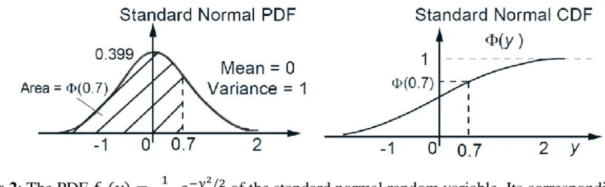
Examples from Lecture 9
Figure 2: The PDF
of the standard normal random variable. Its corresponding CDF,
which is denoted by , is recorded in a table.
A professor's exam scores are approximately distributed normally with mean and standard deviation .
What is the probability that a student scores an or less?
What is the probability that a student scores a or more?
.
What is the probability that a student scores a or less?
.
If your table does not have negatives, use . What is the probability that a student scores between and ?
.
Problem 3. Let and be normal random variables with means and , respectively, and variances and , respectively.
(a) Find and . (b) What is the PDF of . (c) Find .
Solution: (a) is a standard normal, so we have . Also .
(b) By subtracting from its mean and dividing by the standard deviation, we obtain the standard normal.
(c) We have
.
Problem 4. Let be a normal random variable with zero mean and standard deviation . Use the normal tables to compute the probabilities of the events and for .
Solution: Let be the standard normal random variable. We have , so .
From the normal tables we have
Thus , , . We also have
.
Using the normal table values above, we obtain , , .
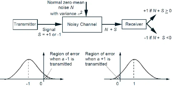
Problem 5. Signal Detection. A binary message is transmitted as a signal that is either or . The communication channel corrupts the transmission with additive normal noise with mean and variance . The receiver concludes that the signal (or ) was transmitted if the value received is (or , respectively); see Fig. 3. What is the probability of error?
Solution: An error occurs whenever is transmitted and the noise is at least so that , or whenever is transmitted and the noise is smaller than so that . In the former case, the probability of error is
.
In the latter case, the probability of error is the same, by symmetry. The value of can be obtained from the normal table. For , we have , and the probability of the error is .