Lecture 11
Systems of random variables
Plan of the lecture:
1. Joint PMFs of Multiple Random Variables 1.1 Joint PMF of two random variables 1.2 Functions of Multiple Random Variables 1.3 More than Two Random Variables
1.4 Conditioning one Random Variable on Another 2. Multiple Continuous Random Variables
2.1 Joint PDF of two random variables
2.2 Conditioning One Random Variable on Another 2.3 Inference and the Continuous Bayes’ Rule 3. Independence
3.1 Summary of Facts About Independent Discrete Random Variables 3.2 Independence of Continuous Random Variables
4. Joint CDFs
5. Covariance and Correlation
1 Joint PMFs of Multiple Random Variables
1.1 Joint PMF of two random variables
Probabilistic models often involve several random variables of interest. For example, in a medical diagnosis context, the results of several tests may be significant, or in a networking context, the workloads of several gateways may be of interest. All of these random variables are associated with the same experiment, sample space, and probability law, and their values may relate in interesting ways. This motivates us to consider probabilities involving simultaneously the numerical values of several random variables and to investigate their mutual couplings. We will extend the concepts of PMF and expectation developed so far to multiple random variables.
Consider two discrete random variables 𝑋 and 𝑌 associated with the same experiment. The joint PMF of 𝑋and 𝑌is defined by
𝑝𝑋,𝑌(𝑥, 𝑦) = 𝑃(𝑋 = 𝑥, 𝑌 = 𝑦)
for all pairs of numerical values (𝑥, 𝑦) that 𝑋 and 𝑌 can take. Here and elsewhere, we will use the abbreviated notation 𝑃(𝑋 = 𝑥, 𝑌 = 𝑦) instead of the more precise notations 𝑃( 𝑋 = 𝑥 ∩ 𝑌 = 𝑦 ) or 𝑃(𝑋 = 𝑥 𝑎𝑛𝑑 𝑌 = 𝑦).
The joint PMF determines the probability of any event that can be specified in terms of the random variables 𝑋 and 𝑌. For example if 𝐴 is the set of all pairs (𝑥, 𝑦) that have a certain property, then
𝑃 𝑋, 𝑌 ∈ 𝐴 = (𝑥,𝑦)∈𝐴𝑝𝑋,𝑌(𝑥, 𝑦).
In fact, we can calculate the PMFs of 𝑋and 𝑌by using the formulas
𝑝𝑋(𝑥) = 𝑝𝑦 𝑋,𝑌(𝑥, 𝑦), 𝑝𝑌(𝑦) = 𝑝𝑥 𝑋,𝑌(𝑥, 𝑦).
The formula for 𝑝𝑋(𝑥) can be verified using the calculation
where the second equality follows by noting that the event {𝑋 = 𝑥} is the union of the disjoint events {𝑋 = 𝑥, 𝑌 = 𝑦} as 𝑦 ranges over all the different values of 𝑌. The formula for 𝑝𝑌(𝑦) is
verified similarly. We sometimes refer to 𝑝𝑋 and 𝑝𝑌 as the marginal PMFs, to distinguish them from the joint PMF.
The example of Fig. 1 illustrates the calculation of the marginal PMFs from the joint PMF by using the tabular method. Here, the joint PMF of 𝑋 and 𝑌 is arranged in a two-dimensional table, and the marginal PMF of 𝑋 or 𝑌 at a given value is obtained by adding the table entries along a corresponding column or row, respectively.
Figure 1: Illustration of the tabular method for calculating marginal PMFs from joint PMFs. The joint PMF is represented by a table, where the number in each square (𝑥, 𝑦) gives the value of 𝑝𝑋,𝑌(𝑥, 𝑦). To calculate the marginal PMF 𝑝𝑋 𝑥 for a given value of 𝑥, we add the numbers in the column corresponding to 𝑥. For example 𝑝𝑋 2 = 6/20. Similarly, to calculate the marginal PMF 𝑝𝑌(𝑦) for a given value of 𝑦, we add the numbers in the row corresponding to 𝑦. For example 𝑝𝑌(2) = 7/20.
1.2 Functions of Multiple Random Variables
𝑝𝑍 𝑧 = 𝑥,𝑦 | 𝑔 𝑥,𝑦 =𝑧 𝑝𝑋,𝑌(𝑥, 𝑦).
Furthermore, the expected value rule for functions naturally extends and takes the form
𝐸 𝑔 𝑋, 𝑌 = 𝑥,𝑦𝑔 𝑥, 𝑦 𝑝𝑋,𝑌(𝑥, 𝑦).
The verification of this is very similar to the earlier case of a function of a single random variable. In the special case where 𝑔 is linear and of the form 𝑎𝑋 + 𝑏𝑌 + 𝑐, where 𝑎, 𝑏, and 𝑐 are given scalars, we have
𝐸[𝑎𝑋 + 𝑏𝑌 + 𝑐] = 𝑎𝐸[𝑋] + 𝑏𝐸[𝑌] + 𝑐.
1.3 More than Two Random Variables
The joint PMF of three random variables 𝑋, 𝑌, and 𝑍is defined in analogy with the above as
𝑝𝑋,𝑌,𝑍(𝑥, 𝑦, 𝑧) = 𝑃(𝑋 = 𝑥, 𝑌 = 𝑦, 𝑍 = 𝑧),
for all possible triplets of numerical values (𝑥, 𝑦, 𝑧). Corresponding marginal PMFs are analogously obtained by equations such as
𝑝𝑋,𝑌 𝑥, 𝑦 = 𝑝𝑧 𝑋,𝑌,𝑍(𝑥, 𝑦, 𝑧) and 𝑝𝑋 𝑥 = 𝑝𝑌 𝑍 𝑋,𝑌,𝑍(𝑥, 𝑦, 𝑧).
The expected value rule for functions takes the form
𝐸 𝑔 𝑋, 𝑌, 𝑍 = 𝑥,𝑦,𝑧𝑔 𝑥, 𝑦, 𝑧 𝑝𝑋,𝑌,𝑍(𝑥, 𝑦, 𝑧),
and if 𝑔is linear and of the form 𝑎𝑋 + 𝑏𝑌 + 𝑐𝑍 + 𝑑, then
Furthermore, there are obvious generalizations of the above to more than three random variables. For example, for any random variables 𝑋1, 𝑋2, … , 𝑋𝑛 and any scalars 𝑎1, 𝑎2, … , 𝑎𝑛, we
have
𝐸[𝑎1𝑋1+ 𝑎2𝑋2+ ⋯ + 𝑎𝑛𝑋𝑛] = 𝑎1𝐸[𝑋1] + 𝑎2𝐸[𝑋2] + ⋯ + 𝑎𝑛𝐸[𝑋𝑛].
Summary of Facts About Joint PMFs
Let 𝑋and 𝑌be random variables associated with the same experiment. – The joint PMF of 𝑋and 𝑌is defined by
𝑝𝑋,𝑌(𝑥, 𝑦) = 𝑃(𝑋 = 𝑥, 𝑌 = 𝑦).
– The marginal PMFs of 𝑋and 𝑌can be obtained from the joint PMF, using the formulas
𝑝𝑋(𝑥) = 𝑝𝑦 𝑋,𝑌(𝑥, 𝑦), 𝑝𝑌(𝑦) = 𝑝𝑥 𝑋,𝑌(𝑥, 𝑦).
– A function 𝑔(𝑋, 𝑌) of 𝑋and 𝑌defines another random variable, and
𝐸 𝑔 𝑋, 𝑌 = 𝑥,𝑦𝑔 𝑥, 𝑦 𝑝𝑋,𝑌(𝑥, 𝑦).
– If 𝑔 is linear, of the form 𝑎𝑋 + 𝑏𝑌 + 𝑐, we have
𝐸[𝑎𝑋 + 𝑏𝑌 + 𝑐] = 𝑎𝐸[𝑋] + 𝑏𝐸[𝑌] + 𝑐.
– The above have natural extensions to the case where more than two random variables are involved.
1.4 Conditioning one Random Variable on Another
𝑝𝑋|𝑌(𝑥|𝑦) = 𝑃(𝑋 = 𝑥|𝑌 = 𝑦).
Using the definition of conditional probabilities, we have
𝑝𝑋|𝑌(𝑥|𝑦) =𝑃(𝑋=𝑥,𝑌=𝑦)𝑃(𝑌=𝑦) =𝑝𝑋 ,𝑌𝑝 (𝑥,𝑦)
𝑌(𝑦) .
Let us fix some 𝑦, with 𝑝𝑌(𝑦) > 0 and consider 𝑝𝑋|𝑌(𝑥|𝑦) as a function of 𝑥. This function is a valid PMF for 𝑋: it assigns nonnegative values to each possible 𝑥, and these values add to 1. Furthermore, this function of 𝑥, has the same shape as 𝑝𝑋,𝑌(𝑥, 𝑦) except that it is normalized by dividing with 𝑝𝑌(𝑦), which enforces the normalization property
𝑝𝑥 𝑋|𝑌(𝑥|𝑦) = 1.
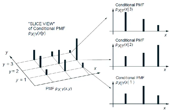
Figure 2 provides a visualization of the conditional PMF.
Figure 2: Visualization of the conditional PMF 𝑝𝑋|𝑌(𝑥|𝑦). For each 𝑦, we view the joint PMF
along the slice 𝑌 = 𝑦and renormalize so that 𝑝𝑥 𝑋|𝑌(𝑥|𝑦)= 1.
The conditional PMF is often convenient for the calculation of the joint PMF, using a sequential approach and the formula
or its counterpart
𝑝𝑋,𝑌(𝑥, 𝑦) = 𝑝𝑋(𝑥)𝑝𝑌|𝑋(𝑦|𝑥).
This method is entirely similar to the use of the multiplication rule.
The conditional PMF can also be used to calculate the marginal PMFs. In particular, we have by using the definitions,
𝑝𝑋 𝑥 = 𝑝𝑦 𝑋,𝑌(𝑥, 𝑦)= 𝑝𝑦 𝑌(𝑦)𝑝𝑋|𝑌(𝑥|𝑦).
This formula provides a divide-and-conquer method for calculating marginal PMFs. It is in essence identical to the total probability theorem, but cast in different notation.
Note finally that one can define conditional PMFs involving more than two random variables, as in 𝑝𝑋,𝑌|𝑍(𝑥, 𝑦|𝑧) or 𝑝𝑋|𝑌,𝑍(𝑥|𝑦, 𝑧). The concepts and methods described above
generalize easily.
2 Multiple Continuous Random Variables p. 125
2.1 Joint PDF of two random variables
We will now extend the notion of a PDF to the case of multiple random variables. In complete analogy with discrete random variables, we introduce joint, marginal, and conditional PDFs. Their intuitive interpretation as well as their main properties parallel the discrete case.
We say that two continuous random variables associated with a common experiment are
jointly continuous and can be described in terms of a joint PDF 𝑓𝑋,𝑌, if 𝑓𝑋,𝑌 is a nonnegative function that satisfies
𝑃 𝑋, 𝑌 ∈ 𝐵 = 𝑋,𝑌 ∈𝐵𝑓𝑋,𝑌(𝑥, 𝑦)𝑑𝑥𝑑𝑦,
𝑃(𝑎 ≤ 𝑋 ≤ 𝑏, 𝑐 ≤ 𝑌 ≤ 𝑑) = 𝑓𝑐𝑑 𝑎𝑏 𝑋,𝑌(𝑥, 𝑦)𝑑𝑥𝑑𝑦.
Furthermore, by letting 𝐵 be the entire two-dimensional plane, we obtain the normalization property
𝑓−∞∞ −∞∞ 𝑋,𝑌 𝑥, 𝑦 𝑑𝑥𝑑𝑦 = 1.
To interpret the PDF, we let 𝛿 be very small and consider the probability of a small rectangle. We have
𝑃(𝑎 ≤ 𝑋 ≤ 𝑎 + 𝛿, 𝑐 ≤ 𝑌 ≤ 𝑐 + 𝛿) = 𝑐𝑐+𝛿 𝑎𝑎+𝛿𝑓𝑋,𝑌(𝑥, 𝑦)𝑑𝑥𝑑𝑦≈ 𝑓𝑋,𝑌(𝑎, 𝑐) ∙ 𝛿2,
so we can view 𝑓𝑋,𝑌(𝑎, 𝑐) as the “probability per unit area” in the vicinity of (𝑎, 𝑐).
The joint PDF contains all conceivable probabilistic information on the random variables 𝑋and 𝑌, as well as their dependencies. It allows us to calculate the probability of any event that can be defined in terms of these two random variables. As a special case, it can be used to calculate the probability of an event involving only one of them. For example, let 𝐴 be a subset of the real line and consider the event {𝑋 ∈ 𝐴}. We have
𝑃 𝑋 ∈ 𝐴 = 𝑃 𝑋 ∈ 𝐴 𝑎𝑛𝑑 𝑌 ∈ (−∞, ∞) = 𝑓𝐴 −∞∞ 𝑋,𝑌(𝑥, 𝑦)𝑑𝑦𝑑𝑥.
Comparing with the formula
𝑃 𝑋 ∈ 𝐴 = 𝑓𝑋(𝑥)𝑑𝑥
𝐴
we see that the marginal PDF 𝑓𝑋 of 𝑋is given by
𝑓𝑋 𝑥 = 𝑓−∞∞ 𝑋,𝑌(𝑥, 𝑦)𝑑𝑦.
𝑓𝑌 𝑦 = 𝑓−∞∞ 𝑋,𝑌(𝑥, 𝑦)𝑑𝑥.
Expectation
If 𝑋 and 𝑌 are jointly continuous random variables, and 𝑔 is some function, then 𝑍 = 𝑔(𝑋, 𝑌) is also a random variable. Let us note that the expected value rule is still applicable and
𝐸 𝑔(𝑋, 𝑌) = 𝑔(𝑥, 𝑦)𝑓−∞∞ −∞∞ 𝑋,𝑌(𝑥, 𝑦)𝑑𝑥𝑑𝑦.
As an important special case, for any scalars 𝑎, 𝑏, we have
𝐸[𝑎𝑋 + 𝑏𝑌] = 𝑎𝐸[𝑋] + 𝑏𝐸[𝑌].
2.2 Conditioning One Random Variable on Another
Let 𝑋 and 𝑌 be continuous random variables with joint PDF 𝑓𝑋,𝑌. For any fixed 𝑦 with
𝑓𝑌(𝑦) > 0, the conditional PDF of 𝑋given that 𝑌 = 𝑦, is defined by
𝑓𝑋|𝑌(𝑥|𝑦) =𝑓𝑋 ,𝑌(𝑥,𝑦)
𝑓𝑌(𝑦) .
This definition is analogous to the formula 𝑝𝑋|𝑌 = 𝑝𝑋,𝑌/𝑝𝑌 for the discrete case.
When thinking about the conditional PDF, it is best to view 𝑦 as a fixed number and consider 𝑓𝑋|𝑌(𝑥|𝑦) as a function of the single variable 𝑥. As a function of 𝑥, the conditional PDF 𝑓𝑋|𝑌(𝑥|𝑦) has the same shape as the joint PDF 𝑓𝑋,𝑌(𝑥, 𝑦), because the normalizing factor 𝑓𝑌(𝑦) does not depend on 𝑥; see Fig. 3. Note that the normalization ensures that
𝑓−∞∞ 𝑋|𝑌(𝑥|𝑦)𝑑𝑥= 1,
Figure 3: Visualization of the conditional PDF 𝑓𝑋|𝑌(𝑥|𝑦). Let 𝑋,𝑌have a joint PDF which is uniform on the set 𝑆. For each fixed 𝑦, we consider the joint PDF along the slice 𝑌 = 𝑦and
normalize it so that it integrates to 1.
To interpret the conditional PDF, let us fix some small positive numbers 𝛿1 and 𝛿2, and condition on the event 𝐵 = {𝑦 ≤ 𝑌 ≤ 𝑦 + 𝛿2}. We have
𝑃(𝑥 ≤ 𝑋 ≤ 𝑥 + 𝛿1|𝑦 ≤ 𝑌 ≤ 𝑦 + 𝛿2) =𝑃(𝑥≤𝑋≤𝑥+𝛿1 𝑎𝑛𝑑 𝑦≤𝑌≤𝑦+𝛿2)
𝑃(𝑦≤𝑌≤𝑦+𝛿2) ≈
𝑓𝑋 ,𝑌(𝑥,𝑦)𝛿1𝛿2
𝑓𝑌(𝑦)𝛿2 = 𝑓𝑋|𝑌(𝑥|𝑦)𝛿1. In words, 𝑓𝑋|𝑌(𝑥|𝑦)𝛿1 provides us with the probability that 𝑋 belongs in a small interval
[𝑥, 𝑥 + 𝛿1], given that 𝑌 belongs in a small interval [𝑦, 𝑦 + 𝛿2]. Since 𝑓𝑋|𝑌(𝑥|𝑦)𝛿1 does not
depend on 𝛿2, we can think of the limiting case where 𝛿2 decreases to zero and write 𝑃(𝑥 ≤ 𝑋 ≤ 𝑥 + 𝛿1|𝑌 = 𝑦) ≈ 𝑓𝑋|𝑌(𝑥|𝑦)𝛿1, (𝛿1 small),
and, more generally,
𝑃 𝑋 ∈ 𝐴 𝑌 = 𝑦) = 𝑓𝐴 𝑋|𝑌(𝑥|𝑦)𝑑𝑥.
Conditional probabilities, given the zero probability event {𝑌 = 𝑦}, were left undefined in earlier lectures. But the above formula provides a natural way of defining such conditional probabilities in the present context. In addition, it allows us to view the conditional PDF 𝑓𝑋|𝑌(𝑥|𝑦) (as a function of 𝑥) as a description of the probability law of 𝑋, given that the event {𝑌 = 𝑦}has occurred.
modeling: instead of directly specifying 𝑓𝑋,𝑌, it is often natural to provide a probability law for 𝑌, in terms of a PDF 𝑓𝑌, and then provide a conditional probability law 𝑓𝑋|𝑌(𝑥, 𝑦) for 𝑋, given any possible value 𝑦of 𝑌.
Having defined a conditional probability law, we can also define a corresponding conditional expectation by letting
𝐸[𝑋|𝑌 = 𝑦] = 𝑥𝑓−∞∞ 𝑋|𝑌(𝑥|𝑦)𝑑𝑥.
The properties of (unconditional) expectation carry though, with the obvious modifications, to conditional expectation. For example the conditional version of the expected value rule
𝐸[𝑔 𝑋 |𝑌 = 𝑦] = 𝑔 𝑥 𝑓∞ 𝑋|𝑌(𝑥|𝑦)𝑑𝑥
−∞
remains valid.
Summary of Facts About Multiple Continuous Random Variables
Let 𝑋and 𝑌be jointly continuous random variables with joint PDF 𝑓𝑋,𝑌.
– The joint, marginal, and conditional PDFs are related to each other by the formulas
𝑓𝑋,𝑌 𝑥, 𝑦 = 𝑓𝑌(𝑦)𝑓𝑋|𝑌(𝑥|𝑦),
𝑓𝑋 𝑥 = 𝑓−∞∞ 𝑌(𝑦)𝑓𝑋|𝑌(𝑥|𝑦)𝑑𝑦.
The conditional PDF 𝑓𝑋|𝑌(𝑥|𝑦) is defined only for those 𝑦for which 𝑓𝑌(𝑦) > 0. – They can be used to calculate probabilities:
𝑃 𝑋, 𝑌 ∈ 𝐵 = 𝑋,𝑌 ∈𝐵𝑓𝑋,𝑌(𝑥, 𝑦)𝑑𝑥𝑑𝑦,
𝑃 𝑋 ∈ 𝐴 = 𝑓𝐴 𝑋(𝑥)𝑑𝑥,
𝑃 𝑋 ∈ 𝐴 𝑌 = 𝑦) = 𝑓𝐴 𝑋|𝑌(𝑥|𝑦)𝑑𝑥.
𝐸 𝑔(𝑋) = 𝑔(𝑥)𝑓−∞∞ 𝑋(𝑥)𝑑𝑥,
𝐸 𝑔(𝑋, 𝑌) = 𝑔(𝑥, 𝑦)𝑓−∞∞ −∞∞ 𝑋,𝑌(𝑥, 𝑦)𝑑𝑥𝑑𝑦,
𝐸[𝑔 𝑋 |𝑌 = 𝑦] = 𝑔 𝑥 𝑓−∞∞ 𝑋|𝑌(𝑥|𝑦)𝑑𝑥,
𝐸[𝑔 𝑋, 𝑌 |𝑌 = 𝑦] = 𝑔 𝑥, 𝑦 𝑓−∞∞ 𝑋|𝑌(𝑥|𝑦)𝑑𝑥.
– We have the following versions of the total expectation theorem:
𝐸 𝑋 = 𝐸 𝑋|𝑌 = 𝑦 𝑓𝑌(𝑦) 𝑑𝑦,
𝐸 𝑔 𝑋 = 𝐸 𝑔 𝑋 |𝑌 = 𝑦 𝑓𝑌(𝑦) 𝑑𝑦,
𝐸 𝑔 𝑋, 𝑌 = 𝐸 𝑔 𝑋, 𝑌 |𝑌 = 𝑦 𝑓𝑌(𝑦) 𝑑𝑦.
2.3 Inference and the Continuous Bayes’ Rule
In many situations, we have a model of an underlying but unobserved phenomenon, represented by a random variable 𝑋 with PDF 𝑓𝑋, and we make noisy measurements 𝑌. The measurements are supposed to provide information about 𝑋 and are modeled in terms of a conditional PDF 𝑓𝑋|𝑌. For example, if 𝑌is the same as 𝑋, but corrupted by zero-mean normally
distributed noise, one would let the conditional PDF 𝑓𝑌|𝑋(𝑦|𝑥) of 𝑌, given that 𝑋 = 𝑥, be normal
with mean equal to 𝑥. Once the experimental value of 𝑌is measured, what information does this provide on the unknown value of 𝑋?
This setting is similar to introduced the Bayes rule and used it to solve inference problems. The only difference is that we are now dealing with continuous random variables.
Note that the information provided by the event {𝑌 = 𝑦} is described by the conditional PDF 𝑓𝑋|𝑌(𝑥|𝑦). It thus suffices to evaluate the latter PDF. A calculation analogous to the original
derivation of the Bayes’ rule, based on the formulas 𝑓𝑋𝑓𝑌|𝑋 = 𝑓𝑋,𝑌= 𝑓𝑌𝑓𝑋|𝑌, yields
𝑓𝑋|𝑌 𝑥 𝑦 =𝑓𝑋 𝑥 𝑓𝑓 𝑌|𝑋(𝑦|𝑥)
𝑌(𝑦) =
𝑓𝑋 𝑥 𝑓𝑌|𝑋(𝑦|𝑥)
𝑓𝑋 𝑡 𝑓𝑌|𝑋(𝑦|𝑡)𝑑𝑡, which is the desired formula.
3 Independence
Let 𝐴 be an event, with 𝑃(𝐴) > 0, and let 𝑋 and 𝑌 be random variables associated with the same experiment.
– 𝑋is independent of the event 𝐴if
𝑝𝑋|𝐴(𝑥) = 𝑝𝑋(𝑥), for all 𝑥,
that is, if for all 𝑥, the events {𝑋 = 𝑥}and 𝐴are independent.
– 𝑋and 𝑌 are independent if for all possible pairs (𝑥, 𝑦), the events {𝑋 = 𝑥}and {𝑌 = 𝑦} are independent, or equivalently
𝑝𝑋,𝑌(𝑥, 𝑦) = 𝑝𝑋(𝑥)𝑝𝑌(𝑦), for all 𝑥, 𝑦.
– If 𝑋and 𝑌are independent random variables, then
𝐸[𝑋𝑌] = 𝐸[𝑋]𝐸[𝑌].
Furthermore, for any functions 𝑓 and 𝑔, the random variables 𝑔(𝑋) and (𝑌) are independent, and we have
𝐸[𝑔 𝑋 𝑌 ] = 𝐸[𝑔 𝑋 ]𝐸[ 𝑌 ].
– If 𝑋and 𝑌are independent, then
var(𝑋 + 𝑌) = var(𝑋) + var(𝑌).
3.2 Independence of Continuous Random Variables
Suppose that 𝑋and 𝑌are independent, that is,
𝑓𝑋,𝑌(𝑥, 𝑦) = 𝑓𝑋(𝑥)𝑓𝑌(𝑦), for all 𝑥, 𝑦.
We then have the following properties.
– We have
𝐸[𝑋𝑌] = 𝐸[𝑋]𝐸[𝑌],
and, more generally,
𝐸[𝑔 𝑋 𝑌 ] = 𝐸[𝑔 𝑋 ]𝐸[ 𝑌 ].
– We have
var(𝑋 + 𝑌) = var(𝑋) + var(𝑌).
4 Joint CDFs
If 𝑋and 𝑌are two random variables associated with the same experiment, we define their joint CDF by
𝐹𝑋,𝑌(𝑥, 𝑦) = 𝑃(𝑋 ≤ 𝑥, 𝑌 ≤ 𝑦).
As in the case of one random variable, the advantage of working with the CDF is that it applies equally well to discrete and continuous random variables. In particular, if 𝑋 and 𝑌 are described by a joint PDF 𝑓𝑋,𝑌, then
𝐹𝑋,𝑌(𝑥, 𝑦) = 𝑃(𝑋 ≤ 𝑥, 𝑌 ≤ 𝑦) = 𝑓−∞𝑥 −∞𝑦 𝑋,𝑌(𝑠, 𝑡)𝑑𝑠𝑑𝑡.
Conversely, the PDF can be recovered from the PDF by differentiating:
𝑓𝑋,𝑌 𝑥, 𝑦 = 𝜕2𝐹𝑋 ,𝑌
𝜕𝑥𝜕𝑦 (𝑥, 𝑦).
More than Two Random Variables
𝑃 𝑋, 𝑌, 𝑍 ∈ 𝐵 = 𝑥,𝑦,𝑧 ∈𝐵𝑓𝑋,𝑌,𝑍(𝑥, 𝑦, 𝑧)𝑑𝑥𝑑𝑦𝑑𝑧,
for any set 𝐵. We also have relations such as
𝑓𝑋,𝑌(𝑥, 𝑦) = 𝑓𝑋,𝑌,𝑍(𝑥, 𝑦, 𝑧)𝑑𝑧,
and
𝑓𝑋(𝑥) = 𝑓𝑋,𝑌,𝑍(𝑥, 𝑦, 𝑧)𝑑𝑦𝑑𝑧.
One can also define conditional PDFs by formulas such as
𝑓𝑋,𝑌|𝑍(𝑥, 𝑦|𝑧) =𝑓𝑋 ,𝑌,𝑍(𝑥,𝑦,𝑧)
𝑓𝑍(𝑧) , for 𝑓𝑍(𝑧) > 0, 𝑓𝑋|𝑌,𝑍(𝑥|𝑦, 𝑧) =𝑓𝑋 ,𝑌,𝑍(𝑥,𝑦,𝑧)
𝑓𝑌,𝑍(𝑦,𝑧) , for 𝑓𝑌,𝑍(𝑦, 𝑧) > 0. There is an analog of the multiplication rule:
𝑓𝑋,𝑌,𝑍(𝑥, 𝑦, 𝑧) = 𝑓𝑋|𝑌,𝑍(𝑥|𝑦, 𝑧)𝑓𝑌|𝑍(𝑦|𝑧)𝑓𝑍(𝑧).
Finally, we say that the three random variables 𝑋, 𝑌, and 𝑍are independent if
𝑓𝑋,𝑌,𝑍(𝑥, 𝑦, 𝑧) = 𝑓𝑋(𝑥)𝑓𝑌(𝑦)𝑓𝑍(𝑧), for all 𝑥, 𝑦, 𝑧.
The expected value rule for functions takes the form
𝐸 𝑔(𝑋, 𝑌, 𝑍) = 𝑔(𝑥, 𝑦, 𝑧)𝑓𝑋,𝑌,𝑍(𝑥, 𝑦, 𝑧)𝑑𝑥𝑑𝑦𝑑𝑧,
and if 𝑔is linear and of the form 𝑎𝑋 + 𝑏𝑌 + 𝑐𝑍, then
Furthermore, there are obvious generalizations of the above to the case of more than three random variables. For example, for any random variables 𝑋1, 𝑋2, … , 𝑋𝑛 and any scalars
𝑎1, 𝑎2, … , 𝑎𝑛, we have
𝐸[𝑎1𝑋1+ 𝑎2𝑋2+ ⋯ + 𝑎𝑛𝑋𝑛] = 𝑎1𝐸[𝑋1] + 𝑎2𝐸[𝑋2] + ⋯ + 𝑎𝑛𝐸[𝑋𝑛].
5 Covariance and Correlation
The covariance of two random variables 𝑋and 𝑌is denoted by cov(𝑋, 𝑌), and is defined by
cov(𝑋, 𝑌) = 𝐸 𝑋 − 𝐸[𝑋] 𝑌 − 𝐸[𝑌] .
When cov(𝑋, 𝑌) = 0, we say that 𝑋and 𝑌are uncorrelated.
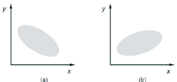
Roughly speaking, a positive or negative covariance indicates that the values of 𝑋 − 𝐸[𝑋] and 𝑌 − 𝐸[𝑌] obtained in a single experiment “tend” to have the same or the opposite sign, respectively (see Fig. 4). Thus the sign of the covariance provides an important qualitative indicator of the relation between 𝑋and 𝑌.
If 𝑋and 𝑌are independent, then
cov 𝑋, 𝑌 = 𝐸 𝑋 − 𝐸 𝑋 𝑌 − 𝐸 𝑌 = 𝐸 𝑋 − 𝐸 𝑋 𝐸 𝑌 − 𝐸 𝑌 = 0.
Thus if 𝑋and 𝑌are independent, they are also uncorrelated. However, the reverse is not true.
The correlation coefficient 𝜌 of two random variables 𝑋 and 𝑌 that have nonzero variances is defined as
𝜌 = cov (𝑋,𝑌)
var (𝑋)var (𝑌).
It may be viewed as a normalized version of the covariance cov(𝑋, 𝑌), and in fact it can be shown that 𝜌ranges from −1 to 1.
If 𝜌 > 0 (or 𝜌 < 0), then the values of 𝑥 − 𝐸[𝑋] and 𝑦 − 𝐸[𝑌] “tend” to have the same (or opposite, respectively) sign, and the size of |𝜌|provides a normalized measure of the extent to which this is true. In fact, always assuming that 𝑋 and 𝑌 have positive variances, it can be shown that 𝜌 = 1 (or 𝜌 = −1) if and only if there exists a positive (or negative, respectively) constant 𝑐such that
𝑦 − 𝐸[𝑌] = 𝑐 𝑥 − 𝐸[𝑋] , for all possible numerical values (𝑥, 𝑦).
The covariance can be used to obtain a formula for the variance of the sum of several (not necessarily independent) random variables. In particular, if 𝑋1, 𝑋2, … , 𝑋𝑛 are random variables with finite variance, we have
var 𝑛 𝑋𝑖
𝑖=1 = 𝑛𝑖=1var 𝑋𝑖 + 2 𝑛𝑖,𝑗 =1cov(𝑋𝑖, 𝑋𝑗) 𝑖<𝑗
.
This can be seen from the following calculation, where for brevity, we denote 𝑋 𝑖 = 𝑋𝑖−
𝐸[𝑋𝑖]:
var 𝑛 𝑋𝑖
𝑖=1 = 𝐸 𝑛𝑖=1𝑋𝑖 2 = 𝐸 𝑛𝑖=1 𝑛𝑗 =1𝑋 𝑖𝑋 𝑗 = 𝑛𝑖=1 𝑛𝑗 =1𝐸 𝑋 𝑖𝑋 𝑗 = 𝑛𝑖=1𝐸 𝑋 𝑖2 +
2 𝑛𝑖,𝑗 =1𝐸 𝑋 𝑖𝑋 𝑗
𝑖<𝑗
= 𝑛 var 𝑋𝑖
𝑖=1 + 2 𝑛𝑖,𝑗 =1cov(𝑋𝑖, 𝑋𝑗) 𝑖<𝑗